Article

Indirect Measurement of Forest Canopy Temperature by Handheld Thermal Infrared Imager through Upward Observation

The Key Laboratory for Silviculture and Conservation of Ministry of Education, Beijing Forestry University, Beijing 100083, China
*
Author to whom correspondence should be addressed.
Remote Sens. 2020, 12(21), 3559; https://doi.org/10.3390/rs12213559
Submission received: 15 September 2020 / Revised: 18 October 2020 / Accepted: 27 October 2020 / Published: 30 October 2020

Abstract

:
The influence of leaf temperature on transpiration, photosynthesis, respiration, and other metabolic activities is critical to plant growth, development, production and distribution. However, traditional measurement of canopy temperature by thermocouples or thermal infrared thermometers is laborious and difficult, especially for tall trees. The recent development of a handheld thermal infrared imager has made it possible to perform high temporal and spatial canopy temperature measurements efficiently. However, the signal recorded by the sensor is often a mixture of radiation from the target and the atmosphere, which must be corrected to get the true temperature. In this study, we propose a ground-based indirect measurement method of canopy temperature by a handheld thermal infrared imager through upward observation. Visible and thermal images are combined to distinguish the canopy pixels and sky pixels. To remove the atmospheric radiation from the sky, an empirical atmospheric model is established, which can perform atmospheric correction accurately and efficiently. To validate the proposed method, we collected canopy temperatures of 36 species of trees with a FLIR T420 thermal infrared imager and compared the estimated temperatures with those directly measured by thermocouples. The accuracy of the corrected canopy temperature has been significantly improved with mean absolute error reduced from 3.73 °C to 0.64 °C. This proposed canopy temperature measurement method can be used to various applications in remote sensing product validation, and ecosystem and forestry studies.

Graphical Abstract

1. Introduction

Leaf energy balance and the resulting leaf temperature are central research themes of biometeorology [1]. The effects of temperature on transpiration, photosynthesis, respiration and other metabolic activities are critical to plant growth, development, production and distribution [2,3,4,5]. On the other hand, canopy controls water and heat exchange through stomatal control of transpiration and architecture, thereby affecting the canopy temperature [6,7]. Due to changes in stomatal conductance, crown and leaf characteristics, canopy temperature will have diurnal and seasonal changes. Most research on the influence of temperature on ecological processes is based on air temperature, but leaf temperature may deviate greatly from the air temperature. In some ecological process models, including the 3-PG forest growth model [8], biogeochemical models [9,10], and ecohydrological models [11], replacing leaf temperature with air temperature will cause deviations in the results of physiological processes that strongly depend on leaf temperature, such as photosynthesis, respiration and transpiration. Therefore, measuring accurate leaf temperature is of great importance for ecological studies.
Previously, thermocouples or thermal infrared thermometers were usually used to measure leaf temperatures [12,13]. The thermocouple directly measures the contact temperature of a point on a leaf [14]; however, it is difficult to obtain the average temperature of the canopy, as well as temperature changes. Thermal infrared thermometers also lack spatial and temporal resolution [15]. Therefore, it is not feasible to record long-term, accurate and continuous canopy temperature with both thermocouple and thermal infrared thermometer. Satellite-based infrared images provide a possibility for large-area and continuous surveys of vegetation status. Various vegetation parameters including canopy temperature [16,17,18] can be extracted from them. Although thermal infrared images taken by satellites can obtain the average temperature of the canopy in a large area within a short time, the spatial resolution, e.g., 100 m for Landsat 8, is still too rough for distinguishing individual tree crowns. The development of thermal infrared sensors, due to their small size and affordable price, has meant that they can be installed on drones and ground-based supporting platforms, making it possible to perform high temporal and spatial infrared measurements at a close range. The thermal infrared sensors mounted on drones can quickly obtain the spatial distribution of the canopy temperature [19,20]. However, each measurement requires a drone flight, which is not applicable to some applications that require high-temporal and continuous monitoring, especially given the fact that the temperatures of the canopy are changing quickly. Using a supporting platform to install the sensor in the study area can solve this problem [1,21]. This method can automatically and continuously obtain the canopy temperature, which can be used to analyze diurnal and seasonal changes.
Currently, thermal infrared measurements are widely used in agriculture. Some work has utilized canopy temperature to characterize stomatal conductance and closure, drought and pest stress [22,23,24,25]. However, most of these studies are conducted in human-dominated environments (laboratory or crop field environments) where some external factors can be controlled, and research in natural systems is relatively uncommon. To monitor the canopy temperature in the natural environment, thermal infrared imagers are usually mounted on cranes or drones, which observe the temperature from the top of the canopy. In this case, the canopy emissivity, the absorption of radiation by the air between the sensor and the target, the atmospheric path radiation and the soil background radiation will all affect the temperature measurement accuracy of the thermal imager. Therefore, some researchers have proposed methods to eliminate this influence by analyzing the interference of these factors on the thermal imager signal [21,26,27,28]. Although there are few studies using a thermal imager for forest monitoring, existing research reveals the great potential of infrared measurement in forestry applications. Scherrer et al. [29] analyzed the influence of canopy characteristics and drought on the canopy temperature of six deciduous tree species using a thermal imager mounted on a helicopter. Aubrecht et al. [21] analyzed the seasonal and diurnal changes of the canopy temperature and the reasons for these changes through three years of continuous thermal infrared observations at two measurement sites (one in a high-temperature deciduous forest and the other in a subalpine coniferous forest). Leuzinger et al. [1] used construction cranes and high-resolution thermal imaging cameras to analyze the spatial and temporal temperature distribution of canopy in mixed deciduous forests in NW Switzerland.
For forest canopy, a more portable method is to perform upward observation from the bottom of the canopy using handheld thermal imagers or sensors mounted on ground-based platforms such as vehicles or brackets [30], which is more operational and lower-cost. The energy received by the thermal imager in this way comes from both canopy and sky. However, the sky temperature is generally lower than the canopy temperature (clear sky temperature <−40 °C) [31], making the measured canopy temperature lower than the actual value. When the sky accounts for a large proportion, the deviation can even reach 9 °C (according to experimental measurement data). Therefore, it is necessary to remove the influence of sky temperature to obtain an accurate canopy temperature. The sky temperature can be obtained from the sky within the field of view (FOV) of the thermal imager [31]. The results measured by this method may be inaccurate because the sky temperature may be outside the calibration range of the thermal imager. It is possible to measure sky temperature by simulating atmospheric downward radiation through a radiation transfer model (RTM), such as LOWTRAN [32] and MODTRAN [33]. This process usually also requires emissivity and atmospheric conditions such as temperature and water-vapor profiles [34,35]. Atmospheric profiles can usually be retrieved from radiosonde data [36] or from atmospheric reanalysis data, such as the National Centers for Environmental Prediction (NCEP) Global Data Analysis System product and the fifth generation of the European Centre for Medium-Range Weather Forecasts (ECMWF) atmospheric reanalyses of the global climate (ERA5) [37]. However, this method may be impractical for real-time applications because the RTM may be slow. Therefore, establishing an atmospheric correction model that takes into account both accuracy and computational efficiency is of great significance, especially for long-time series thermal infrared image analysis.
This paper proposes a method to measure canopy temperature from ground-based thermal infrared imagers. Visible and thermal images are combined to segment vegetation pixels from thermal images, and a fast atmospheric correction model in the 7–13 μm is established to correct the atmospheric path radiation.

2. Materials and Methods

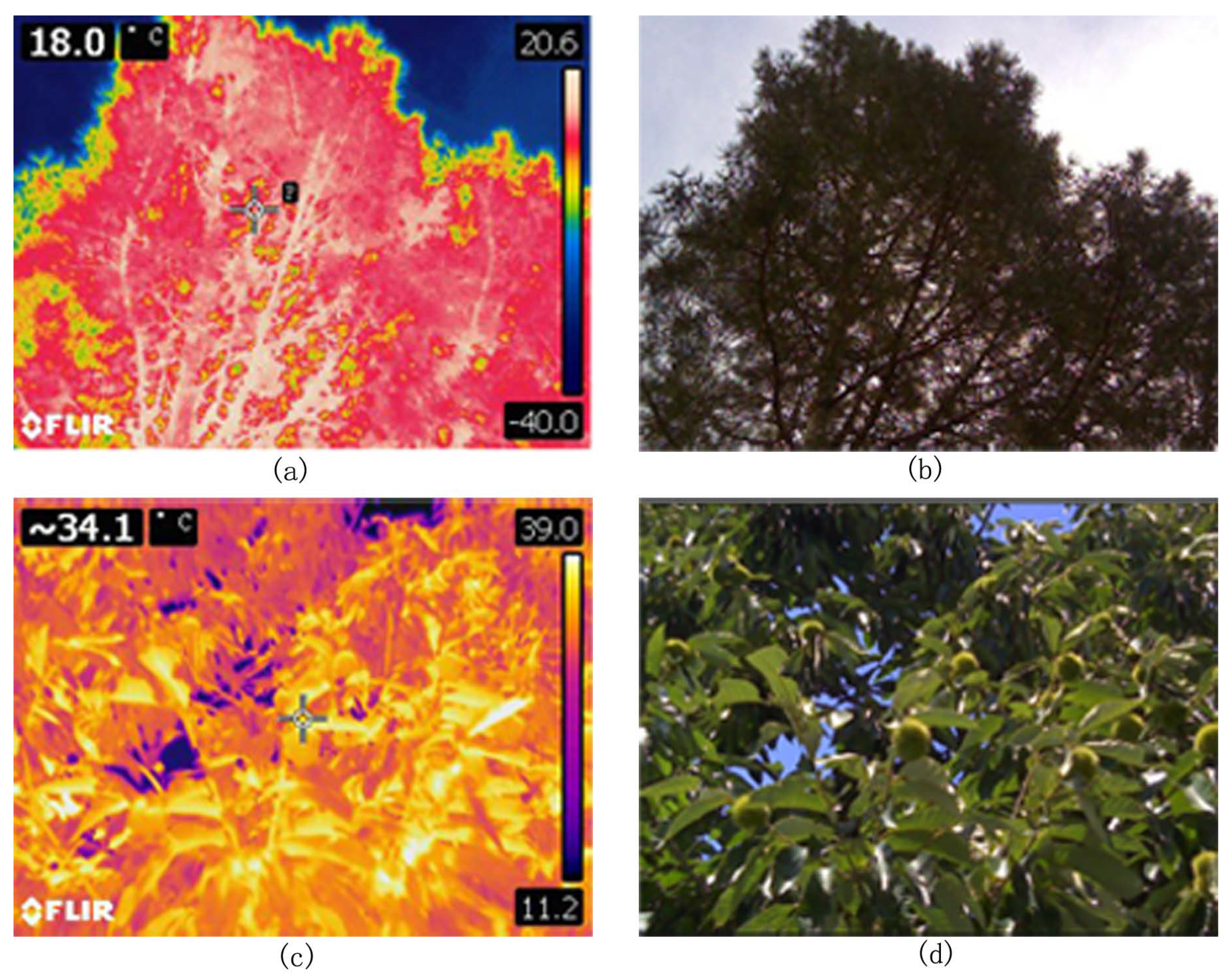
2.1. Thermal Infrared Image

Individual trees used for temperature measurement were located in two areas: one was China’s Beijing Forestry University (40°00′N, 116°20′E), the other was Yuanqiao Town, Huangyan District, Taizhou City, Zhejiang Province (28°31′N, 121°15′E). A total of 56 individual trees were measured, including 36 tree species (Table A1). All thermal infrared images in this study were acquired in clear and cloudless weather using a FLIR T420 handheld thermal imager (7.5–13 μm) with a resolution of 320 × 240 pixels. This imager also simultaneously captures a corresponding visible image along the thermal image. We stood on the ground holding a FLIR T420 thermal imager (about 1.6 meters above the ground) and took thermal infrared images in an upwards direction. The shooting angle was estimated by the tree height and the horizontal distance of the shooting point from the tree.
Figure 1 shows example images taken by the FLIR T420 thermal imager and from the visible images, sky pixels and canopy pixels can be clearly distinguished. Figure 1a was the thermal infrared image of Pinus bungeana Zucc. et Endi. The temperature range was −40.0–20.6 °C. From this picture, we can see that the sky temperature has exceeded the temperature measurement range of the thermal imager. It is no longer possible to use a thermal imager to measure the sky temperature.

2.2. Thermocouple Temperature
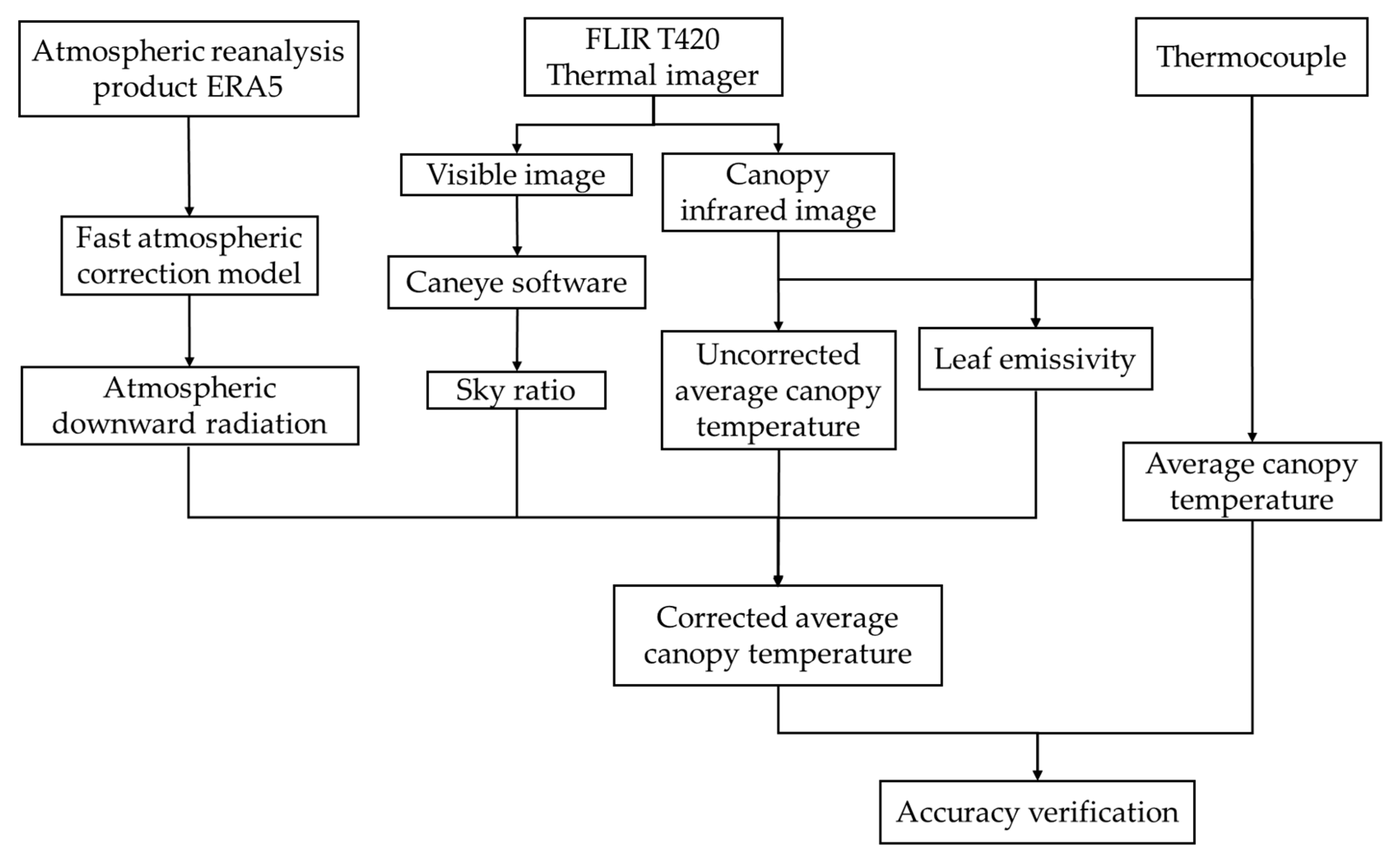
In the canopy photographed by thermal infrared imager, five leaf points were randomly selected, and the contact temperatures were measured by a thermocouple. For tall trees, a ladder was used, instead of picking off the leaves, to ensure a more accurate measurement. The average value of leaf temperatures measured by the thermocouples was taken as the true average temperature of the canopy.

2.3. Methods

Figure 2 shows the main processes of the method, which includes: (1) thermal imager temperature correction and (2) establishment of fast atmospheric correction model.

2.3.1. Canopy Temperature Measurements
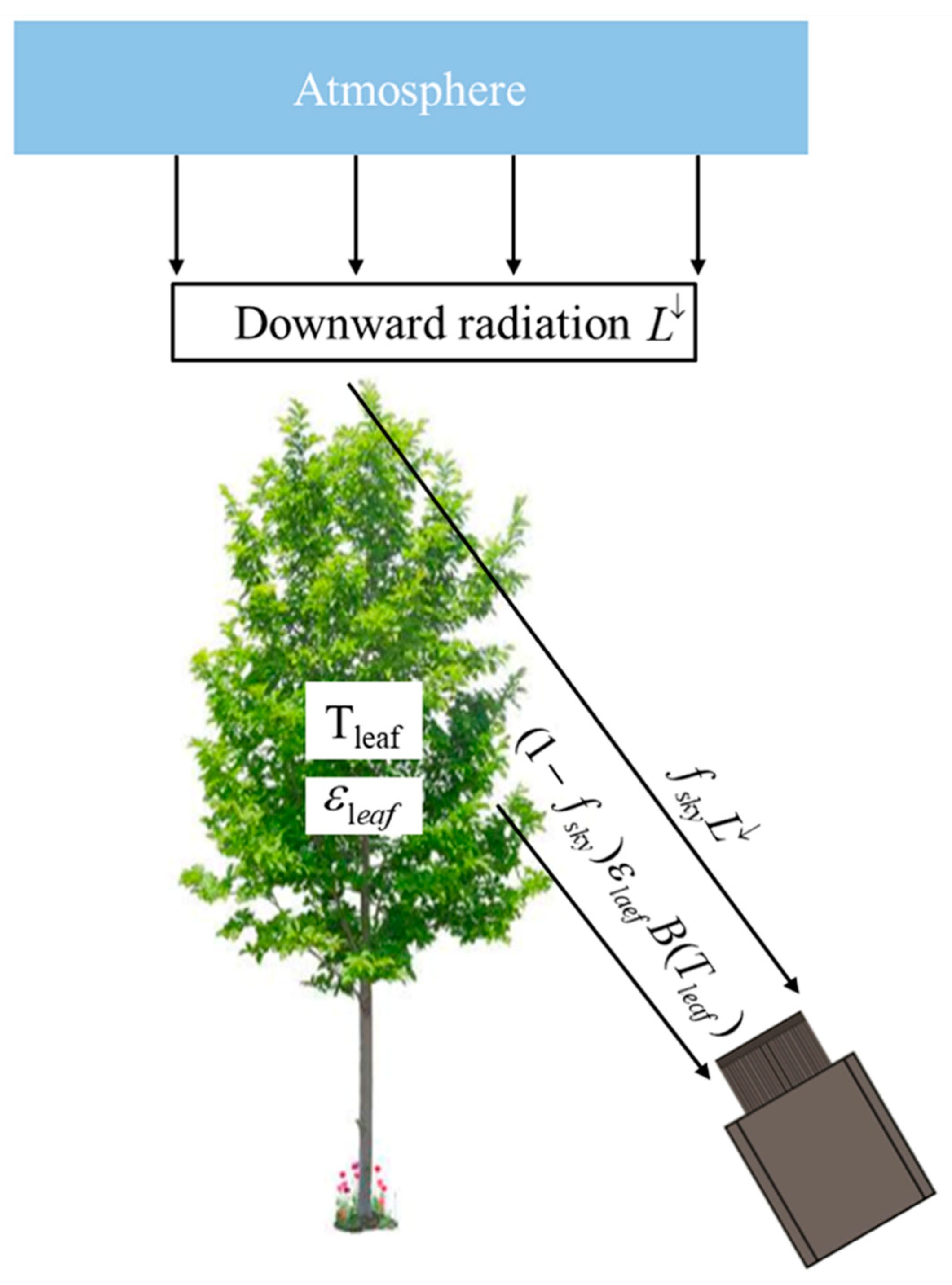
Theory

The emissivity of leaves is generally high in the thermal infrared band [38,39,40], so the transmittance of the leaves is very close to 0. The radiation obtained by upward observation of the canopy is the sum of the atmospheric downward radiation and the target radiation. As shown in Figure 3, the total energy received by the sensor comes from the atmospheric downward radiation penetrating the canopy gaps and the canopy radiation, which can be expressed as
B ( T B ) = f s k y L + ( 1 f s k y ) ε B ( T R ) ,
where B ( T B ) is the energy received by the thermal imager, which is calculated from the measured brightness temperature T B according to Stefan-Boltzmann law; f s k y is the proportion of the sky in the FOV; T R is the true canopy temperature which needs to be solved. B ( T R ) represents the energy radiated by the black body with the same temperature as the canopy, which can be calculated by inverting Equation (1), which gives
B ( T R ) = [ B ( T B ) f s k y L ] / ( ε - f s k y ε ) ,
Then, the true canopy temperature can be calculated by
T R = B ( T R ) σ 4 ,
where σ is the Stefan-Boltzmann constant and the value is about 5.670 × 10⁻⁸ W/ (m2·K4).
When the sky temperature exceeds the range of the thermal imager (clear sky <−40 °C), the thermal imager cannot be used to measure the sky brightness temperature. Therefore, we simulate the atmospheric downward radiation through the radiative transfer model and real-time atmospheric profile data [41,42,43].

Emissivity

Emissivity is the ratio of energy radiated from a material’s surface to that radiated from a blackbody at the same temperature and wavelength and under the same viewing conditions. However, radiation is detected by thermal infrared sensors by the sum of radiation from the target, emitted by the surroundings and atmospheric radiation [44]. Therefore, in order to control the influence of the surrounding environment, emissivity measurements were performed in a black box. We used a branch shear to cut leaves and spread them in the black box. The emissivity of the thermal imager was adjusted to 1 to measure the leaf temperature. At the same time, a thermocouple was used to measure the leaf temperature at five random points. The emissivity calculation formula is as follows:
ε = B ( T B ) / B ( T M ) ,
where T B and T M are the leaf temperature measured by the thermal imager and thermocouple respectively. B ( T B ) and B ( T M ) are calculated by the Stefan-Boltzmann law.

Sky Ratio f s k y

The sky ratio f s k y was calculated using Caneye software [45]: import the visible image of the corresponding area of the canopy thermal infrared image into the Caneye, separate the canopy and sky pixels, and calculate the proportion of sky pixels. The f s k y calculation formula is as follows:
f s k y = n s k y n ,
where n s k y is the number of sky pixels; and n is the total number of pixels.

Atmospheric Downward Radiation

If the atmosphere is divided into several layers, then the atmospheric transmittance of each layer, combined with the temperature profile, can be used to calculate atmospheric downward radiation. Atmospheric downward radiation received by the sensor is a cumulative summation of radiance from all layers [46]. The atmospheric downward radiation of each layer can be calculated by the following formula:
L λ , i = ε λ , i L B B ( λ , i ) + τ λ , i L λ , i + 1 ,
where λ is wavelength; L λ , i is atmospheric downward radiation at a layer; L B B ( λ , i ) is the blackbody radiance of each atmospheric layer; i is the ith layer of atmosphere, and the numbering starts from the bottom atmosphere; ε λ , i is the atmospheric emissivity, since the sum of transmittance, reflectivity and emissivity is 1, where ε λ , i is replaced by (1 − τ λ , i ).
Atmospheric downward radiation of the thermal imager is calculated by convolution of spectral downward radiation and sensor spectral response function [47].
L c = λ 1 λ 2 L λ f ( λ ) d λ / λ 1 λ 2 f ( λ ) d λ ,
By establishing a fast atmospheric correction model, combined with real-time atmospheric profile data, we can quickly calculate the atmospheric downward radiation during the observation time of the thermal imager. The real-time atmospheric profile data used atmospheric reanalysis project ERA5. Atmospheric profile data was divided into 16 layers and inputted into the fast atmospheric correction model.

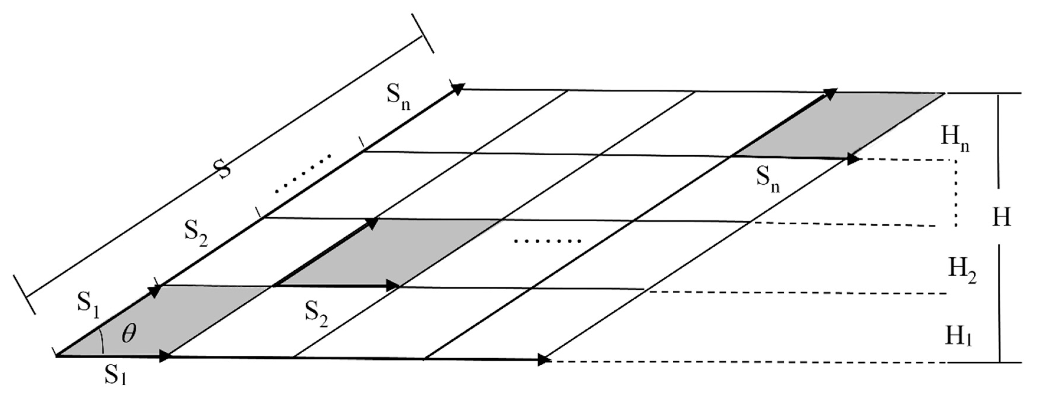
2.3.2. Fast Atmospheric Correction Model

In the 7–13 μm, water vapor and ozone are the major atmospheric absorption components that have a significant effect on radiation transmission (Figure 4a). According to the Beer-Lambert law, the total transmittance is the product of the transmittance of each attenuation component. Therefore, the atmospheric transmittance in 7–13 μm can be approximated as the product of water vapor transmittance and ozone transmittance (Figure 4b).

Water Vapor Continuum Absorption

Water vapor continuum absorption in the 8–13 μm is modelled by a temperature-compensated water vapor continuum function proposed by Roberts [48]. The function can be in terms of path length [48], or in terms of pressure as demonstrated by Price [49]. We divide the atmosphere into several layers, and the atmospheric transmittance of each layer is calculated by the function proposed by Price.
As can be seen in Figure 4c, there is a strong absorption peak within 7–8 μm. Within 7–7.5 μm, the water vapor continuous absorption transmittance is 0. Within 7.5–8 μm, the water vapor continuous absorption transmittance can be approximated by a linear function.
τ w , λ = ( τ w , 8 μ m / 0 . 5 ) ( λ 7 . 5 ) ,
Assuming that the water vapor continuum absorption in each layer is equal in the 7.5–8 μm, the water vapor continuous absorption transmittance in each layer can be expressed as:
τ w ( i ) = τ w , λ ( 1 / n ) ,
where n is the number of atmospheric layers.

Water Vapor Band Type Absorption

Band type absorption is usually calculated by line-by-line integration using molecular absorption lines in the HITRAN database [50]; however, this method is complicated to use. In this paper, a simpler method is proposed. The attenuation ability of water vapor band type absorption is represented by extinction coefficient, and its relationship with transmittance is as follows:
τ W b = exp ( ρ h ) ,
where h is the path length, km; and ρ is the extinction coefficient, km−1.
The shape of the water vapor absorption spectrum is fixed, and the absorption strength is related to the water vapor content and the path length. Therefore, taking the water vapor extinction coefficient of the known water vapor pressure component as a reference, the relationship between water vapor band type absorption and water vapor pressure component can be used to calculate the water vapor extinction coefficient at any water vapor pressure component. This paper used the water vapor extinction coefficient calculated by Modtran as a reference, where the water vapor pressure component is 0.778 kPa (sea level of 1976 U.S. Standard). The extinction coefficient of any atmosphere is calculated as follows:
ρ λ = a ρ λ ,
where ρ λ is the extinction coefficient of the reference atmosphere, km−1; λ is the wavelength, μm; a is a coefficient related to water vapor pressure component, and the formula is as follows:
a = [ b ln ( e ) + c ] e ,
where e is the water vapor pressure component, kPa; and b, c are parameters. According to the six atmospheric profiles from Modtran, the acceptable values of the parameters were determined by trial and error, b = −0.21 kPa−2, c = 0.61 kPa−1.

Horizontal Path Ozone Absorption

The ozone transmittance is linked to the path length and the ability of ozone to attenuate infrared radiation. The attenuation of infrared radiation by ozone is represented by the extinction coefficient. The ozone transmittance can be calculated as follows:
τ H = exp ( є f ( h ) ) ,
where τ H is the ozone transmittance; є is the ozone extinction coefficient, km−1; and f ( h ) is the power function of the path length, km.
The ozone transmittance is related to the wavelength and ozone column density. Therefore, the ozone extinction coefficient was established as a function of a wavelength-dependent exponential term and a primary term associated with the ozone column density. The formula is as follows:
є = [ a + b exp ( c / λ ) ] ( d + f φ ) ,
where λ is the wavelength, μm; є is the extinction coefficient of ozone, km−1; φ is the ozone column density, atm cm/km; and a, b, c, d, f are parameters. We stratified the atmospheric profile of Mid-Latitude Summer at 1 km intervals and fitted the ozone transmittance of 9.4–9.8 μm with Modtran. When h = 1, f ( h ) = 1, so τ H = exp ( є ) . According to the results of ozone transmittance, ozone density and wavelength, each coefficient was fitted, where a = 0.00265 km−1, b = −1.3 km−1, c = 63 μm, d = 1.6, f = 9961.415 (atm cm/km)−1.
At high altitudes, the width of the absorption line is narrowed due to the decrease in atmospheric pressure as the height increases. When passing through the same distance, ozone absorption becomes smaller and the transmittance increases. This phenomenon is not significant when the ozone content is low (Table 1). Therefore, the path function was established as a power function related to the pressure and ozone column density, and the formula is as follows:
f ( h ) = h a ( φ / P ) + b ,
where f ( h ) is the path function, km; h is path length, km; φ is the ozone column density, atm cm/km; P is atmospheric pressure, kPa; and a, b are parameters. According to the data in Table 1, the parameters were obtained by fitting, where a = −49.35 kPa (atm cm/km)−1, b = 0.9160.

Slant Path Ozone Absorption

The ozone content of the atmosphere is very small, and it is mainly located in the spatial range of 10–40 km, especially concentrated at the height of 20–30 km. For high altitudes above 60 km, the effect of ozone on radiation transmission is negligible.
On the slant path, the atmosphere can be divided into several layers, and each layer of the atmosphere can be approximated as a uniform distribution. The slant path is shown in Figure 5, where S is the slant path length and θ is the sensor angle. The ozone transmittance on the slant path is equal to the product of the ozone transmittance of each layer, i.e., τ S = i = 1 n τ S ( i ) . In the horizontal path, the ozone density and atmospheric pressure are constant, so the ozone extinction coefficient and the path function are equal in any region. Horizontal ozone transmittance of the path length S at each layer is τ H ( i ) , and the ozone transmittance of path length S i can be calculated as τ H ( i ) ( S i ) = [ τ H ( i ) ] S i / S . The ozone transmittance of each layer on the slant path is equal to the ozone transmittance of the same length on the horizontal path, i.e., τ S ( i ) = τ H ( i ) ( S i ) . The sensor angle is θ and the slant path length is S i = H i sec θ . Therefore, the expression of ozone transmittance of each layer is:
τ S ( i ) = { exp { [ 0.00265 1.3 exp ( 63 / λ ) ] ( 1.6 + 9961.415 φ i ) ( H sec θ ) ( 49.35 φ i / P i + 0.916 ) >} >} H i sec θ / H sec θ ,

Model Verification

The six atmospheric profiles of the Modtran were divided into 32 layers, and the atmospheric transmittance of the sensor with angles of 0°, and 75° were fitted, respectively. The model accuracy was verified by comparing with Modtran computed transmittances.
The results of the atmospheric transmittance verification are presented in Figure 6. In the 7.5–9.3 μm, the error increased with increased angle, especially for profiles with less water vapor content. The source of the deviation is due to the absorption of non-steam components such as aerosols and CO2, which are components of the Modtran model, but are not considered in the empirical model.
In the 9.3–13 μm, the atmospheric transmittance curves of the two sensor angles of the six atmospheric profiles were consistent with the Modtran fitted curves.

Model Calibration

Due to absorption by non-steam constituents, there is systematic error between the empirical model and the Modtran. Therefore, with reference to the adjustment method of French et al. [35], an absorption term was added to the water vapor continuous extinction coefficient in the 8–9.3 μm:
σ a d j , i = σ i + k / n e i / l ,
The term k represents the total absorption caused by the non-steam component. Since the vertical distribution of these components cannot be known, it is assumed that these components are evenly distributed among the “n” atmospheres. The n is atmospheric pressure difference from bottom to top of the atmosphere, Pa. The role of item l is to reduce the absorption compensation as the water vapor density increases. The acceptable values of the coefficients k and l were determined by trial and error, where k = 0.0891 (Pa−1. Pa), l = 600000 (kPa.Pa).

2.3.3. Accuracy Verification

Accuracy Verification of the Fast Atmospheric Correction Model

Taking Modtran as a reference, we used the atmospheric profile database SeeBorV5.0 [51] for verification. Randomly selected atmospheric profiles including 797 Tropical, 989 Mid-Latitude Summer, 705 Mid-Latitude Winter, 903 Sub-Arctic Summer and 250 Sub-Arctic Winter were divided into 34 layers and input into the empirical model to calculate the atmospheric transmittance and downward radiation of the FLIR T420 thermal imager. The statistical criteria used were the coefficient of determination (R2) and the root mean square error (RMSE), set forth by formulas (18) and (19).

Accuracy Verification of Canopy Temperature Extracted by Thermal Imager

The leaf temperature measured by the thermocouple is used as the real canopy temperature to calculate the accuracy of the canopy temperature extracted by the thermal imager. In order to remove the errors of the instrument, the instrument needs to be calibrated before the experiment. The emissivity of water is approximately 1. We used a thermocouple and FLIR T420 thermal imager to measure the temperature of ice-water mixture (real temperature 0 °C) and boiling water (real temperature 100 °C). The measured temperature and the real temperature were linearly fitted to calibrate the measured temperature of the instrument. The statistical criteria used were the root mean square error (RMSE) and mean absolute error (MAE), set forth by formulas (19) and (20).
R 2 = [ i = 1 n ( y p , i y ¯ p ) ( y m , i y ¯ m ) ] 2 i = 1 n ( y p , i y ¯ p ) 2 i = 1 n ( y m , i y ¯ m ) 2 ,
R M S E = [ i = 1 n ( y p , i y m , i ) 2 n ] 0.5 ,
M A E = 1 n i = 1 n | y p , i y m , i | ,
where y p , i and y m , i are the ith predicted and measured value, respectively, y ¯ p and y ¯ m are the mean of the predicted and measured value, respectively, and n is the number of the data.

3. Results

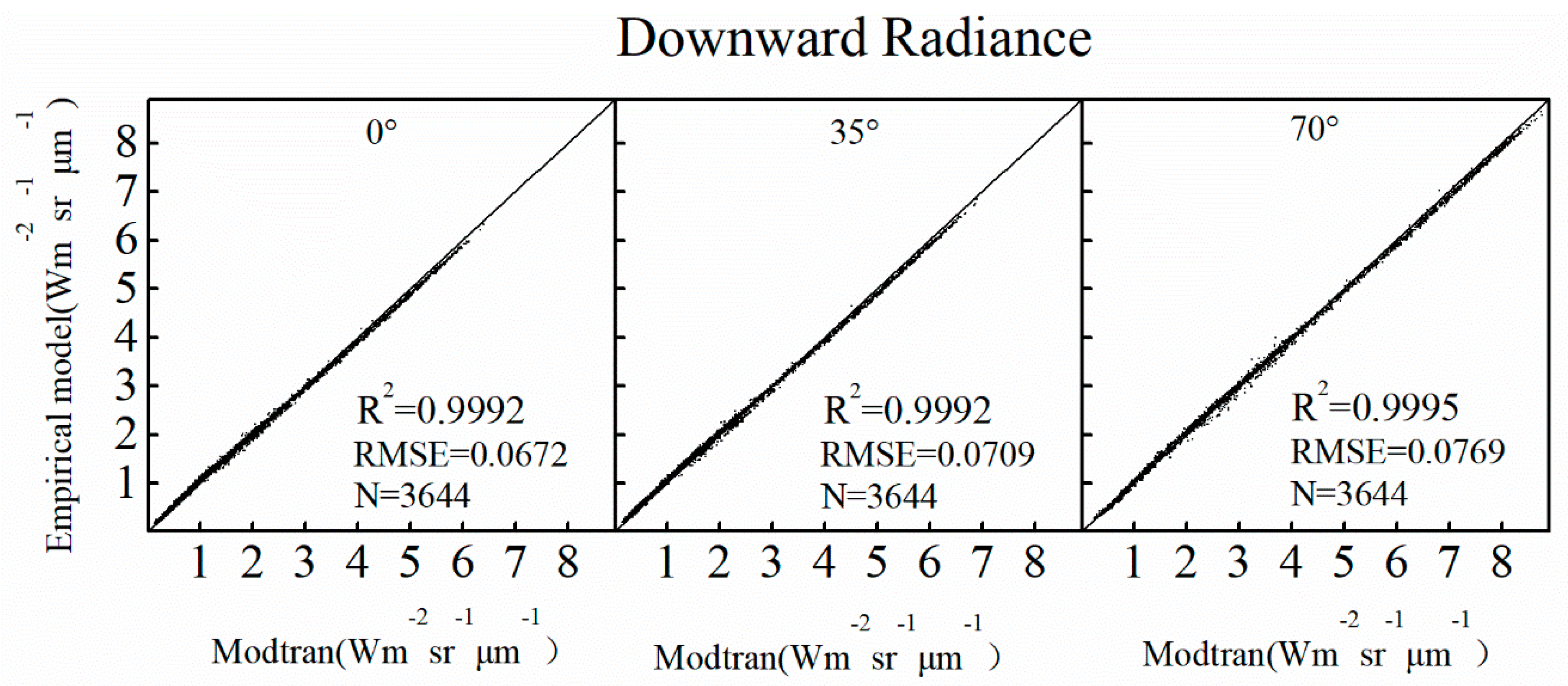
3.1. Accuracy of the Fast Atmospheric Correction Model

Figure 7 shows the comparison of the transmittance results simulated by the calibrated empirical model and Modtran. The absolute error fluctuates around 0, basically at 0.1. But within 7.5–8.2 μm, the transmittance deviation was relatively large, and the absolute value reached 0.3, especially for the profile with less water vapor content. For the error curves of four sensor angles, the difference was not obvious when the angle was within 50°. However, when the sensor angle reached 75°, the error of the profile with higher atmospheric water vapor content decreased, and the error of the profile with lower atmospheric water vapor content increased.

3.2. Accuracy of Empirical Model Applied to FLIR T420 Thermal Imager

Comparison between Modtran and the empirical model-derived atmospheric transmittance and downward radiance for FLIR T420 thermal imager is shown in the Figure 8 and Figure 9. A good agreement was achieved between Modtran and the empirical model-derived transmittance in three sensor angles (0°: R2 = 0.9956, RMSE = 0.0150; 35°: R2 = 0.9960, RMSE = 0.0150; 70°: R2 = 0.9841, RMSE = 0.0268). Modtran and the empirical model-derived atmospheric downward radiance showed good agreement (0°: R2 = 0.9992, RMSE = 0.0672; 35°: R2 = 0.9992, RMSE = 0.0709; 70°: R2 = 0.9995, RMSE = 0.0769). We used the same computer (Intel Core i5-8265U CPU @1.6GHz 1.8GHz, 8GB RAM, Windows 10) to evaluate the computation speed of atmospheric correction for Modtran and the empirical model. Multiple trials showed that the empirical model was at least five times faster than Modtran. For example, the empirical model analysis of 989 profiles with 34 layers of FLIR T420 thermal imager took ~300 s while Modtran took ~1800 s.

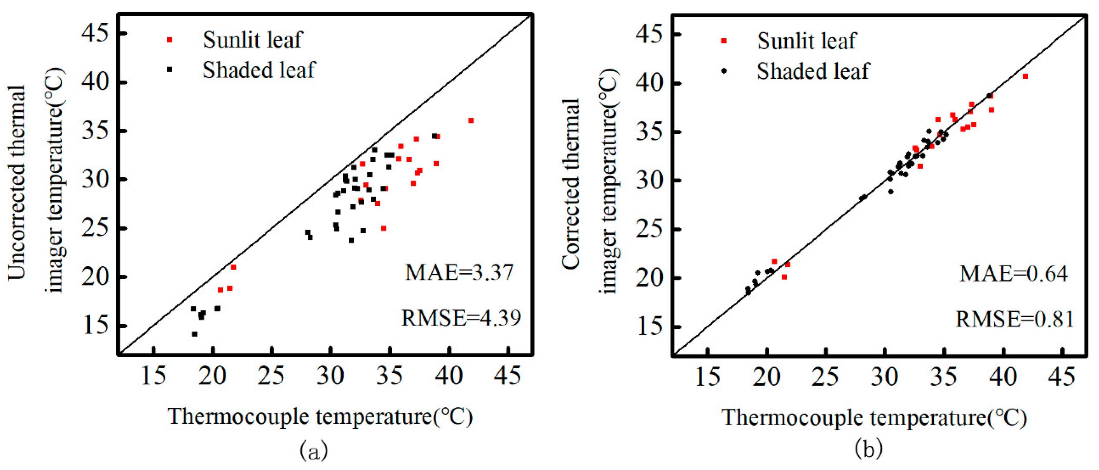
3.3. Accuracy of the Canopy Temperature Extracted by the Thermal Imager

Figure 10 shows the accuracy of the proposed temperature correction method. It can be seen that the accuracy was greatly improved compared with uncorrected measurements (without atmospheric correction), and the mean absolute error was reduced from 3.73 °C to 0.64 °C. Table 2 shows the influence of sunlit and shaded canopies on the canopy temperature extracted by thermal imager. The accuracy of canopy temperature extraction of sunlit canopies was lower than that of shaded canopies (Sunny: MAE = 0.93 °C, RMSE = 1.10 °C; Shady: MAE = 0.49 °C, RMSE = 0.61 °C).

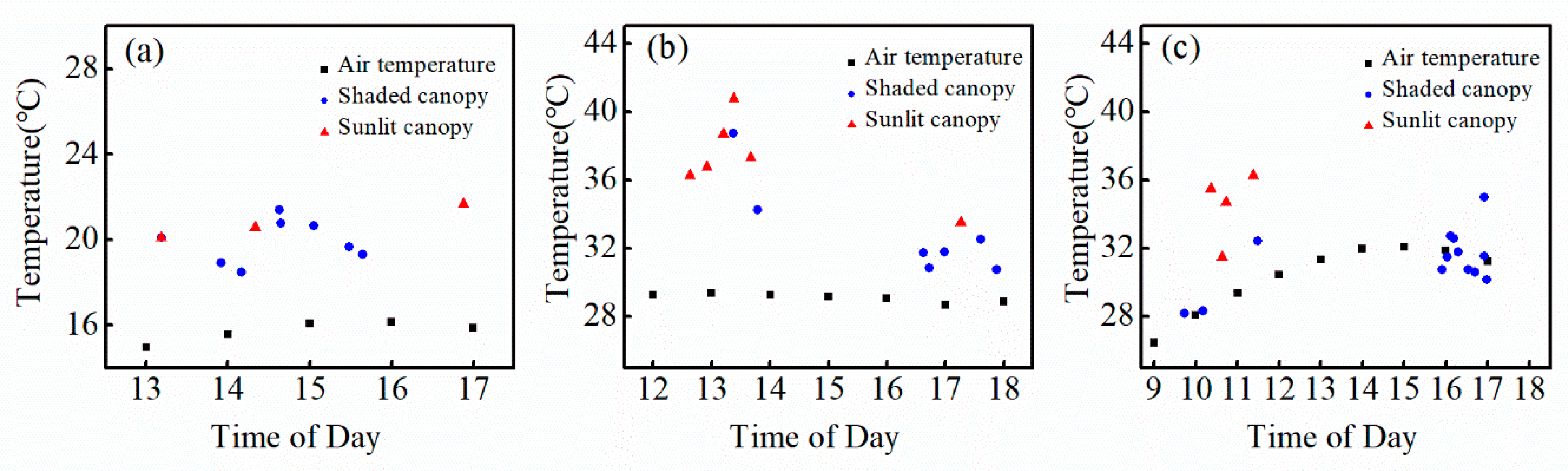
3.4. Canopy Temperatures

Figure 11 shows the difference between canopy temperature and air temperature. Figure 11a is the canopy temperature measured at Beijing Forestry University on 5 October 2019. From 13:00 to 17:00, the canopy temperature was about 4 °C higher than the air temperature. Figure 11b is the data obtained in Yuanqiao Town on 1 August 2020. During the period from 12:00–14:00, the canopy temperature overshot the air temperature by 8 °C, while at 17:00–18:00, the canopy temperature was only 3 °C higher. In addition, the difference between the temperature of the sunlit canopy and the air temperature was larger than that of the shaded canopy. Figure 11c is the data obtained in Beijing Forestry University on 25 August 2020. From 10:00–11:30, there was no significant difference between the shaded canopy temperature and the air temperature, and the sunlit canopy temperature was 5 °C higher than the air temperature. Between 16:00–17:00, air temperature was an approximation of the average canopy temperature.

4. Discussion

In this paper, we proposed an indirect measurement method for canopy temperature by a handheld thermal infrared imager through upward observation. This method improves efficiency while ensuring accuracy, making it of greater application value in forestry. For example, its high efficiency can provide a feasible and simple way for continuous monitoring of canopy temperature. Indirect measurement reduces the difficulty of measuring the canopy temperature, and the obtained accurate results can be used as ground verification data for remote sensing products.

4.1. Method Accuracy

Model verification indicates that the fast atmospheric correction model was in good agreement with the MODTRAN simulation results. Many studies have proposed methods to simplify RTM, including simplification of the radiation transmission process through empirical equations [35,46], correlated-k model [52], or neural networks [53]. The methods proposed in [35,46] are suitable for MODIS and GOES 8 satellite, but not suitable for other thermal infrared channels. However, the model proposed in this paper can be applied to the thermal infrared channels in the range of 7–13 μm. When this model is applied to the FLIR T420 thermal imager, the model has precise atmospheric correction and high computational efficiency. For other thermal infrared sensors including MODIS, Landsat8, VIIRS, similar good results should be obtained. The applicability of the model can be further verified in the follow-up. Although the neural network method proposed in [53] achieved accurate results and was 103 times faster than MODTRAN, inherent limitations to neural networks were not addressed. A long time is needed to train the neural network before use. For example, the network used in [53] took six days to train, but this is fast for most neural networks. In addition, the underlying processes are not clear, and the user may not readily have access to the underlying architecture. However, the atmospheric correction model proposed in this paper is an empirical equation that can be understood and used easily.
The accuracy of the corrected canopy temperature was significantly improved. In addition, we found that the error of the sunlit canopy temperature was greater than the shaded canopy. The main reason is that, when the canopy is irradiated by the sun, shadows will appear on the canopy, which makes the canopy temperature uneven. It is difficult to measure the average temperature of the canopy with a thermocouple. However, thermal imager observation provides a convenient and quick method to obtain the average temperature and temperature change of the canopy [21].

4.2. Influencing Factors of Thermal Imager Measurement

Factors that affect the measured temperature include emissivity, sky ratio and atmospheric downward radiation. The leaf emissivity can be obtained from the literature [39,40,54] or with the measurement method proposed in this paper. However, when calibrating the emissivity of the thermal imager, we cannot simply use the leaf emissivity as the canopy emissivity. When a single pixel contains multiple leaves, the emissivity of the canopy is close to 0.99 [55]. The main reason is that, due to multiple scattering, almost all of the incident thermal radiation is absorbed by the canopy. This study is of close-range measurement, which ensures that most of the pixels are within one leaf. Therefore, it is appropriate to use the leaf emissivity as the canopy emissivity.
The atmospheric downward radiation (sky temperature) is obtained based on the atmospheric correction model and real-time atmospheric profile simulation, but the model does not consider atmospheric scattering and reflection. When clouds are present, they enhance atmospheric downward radiation [56]. Using the method described in the paper to calculate atmospheric downward radiation will produce a large deviation. However, we can combine the method of measuring sky temperature with a thermal imager, because the cloudy sky temperature is within the temperature measurement range of the thermal imager [31].
The sky ratio is also a key factor for the thermal imager to accurately extract the canopy temperature. The main source of sky ratio error is the inability to accurately distinguish the sky and canopy pixels in the area where the canopy and sky meet, especially on conifers with smaller leaves. When the canopy leaves are leathery, sunlit canopy will appear as specular reflection, and this will appear as white in the visible image. Such pixels will also be misclassified as the sky in the Caneye software.

4.3. Advantages and Limitations of the Proposed Method

The canopy temperature measurement method proposed in this paper is suitable for sensors (working band within 7–13 μm) for observation from the bottom of the canopy. With the development of thermal infrared sensors, automatic recording of thermal infrared images has been realized [21]. By fixing the sensor in the sample plot with a bracket, it can realize automatic long-term continuous acquisition of thermal infrared images. However, for research that requires a large number of images, it is impractical to use strict RTM directly for atmospheric correction. The fast atmospheric correction model proposed in this paper serves as an alternative to save time and computational resources.
Compared with drone observation, this method has some advantages, as well as limitations. Using drone observation can quickly obtain the distribution of canopy temperature in an area, and the observation area is flexible and unrestricted [19,20]. However, it is difficult to achieve long-term and high-temporal monitoring because each observation requires a drone flight. Although the coverage of the image taken by the handheld camera is small and it is difficult to analyze the spatial change of the canopy temperature, the proposed method is more flexible in time scale and can be used to analyze diurnal and seasonal changes. The comparison results of canopy temperature and air temperature are consistent with the research of Smith et al. [57] and Doughty et al. [58], which proves that this method can be used for time series analysis of canopy temperature. The method of mounting the sensor on the crane is similar to the method proposed in this paper, and can be used for long-term monitoring [1,21]. However, this method is expensive and requires specialized workers to build the crane. Once installed, it is not easy to disassemble and change the position. In contrast, the method proposed in this paper is inexpensive and simple to operate. The platform used to install the sensor, such as a bracket, is easier to move.

5. Conclusions

In this study, we have proposed a method of using a handheld thermal imager to obtain canopy temperature through upward observation. The canopy temperature is corrected by analyzing the interference factors of the signal recorded by the thermal imager, including atmospheric influence and canopy characteristics. The results show that this method is completely feasible for the accurate measurement of canopy temperature. In addition, we achieved rapid acquisition of atmospheric downward radiation by establishing a fast atmospheric correction model combined with real-time atmospheric profile. The observation method has acceptable accuracy and fast processing speed, combined with automatic image recording technology, and can realize long-term continuous monitoring of canopy temperature.

Author Contributions

Data curation, A.S.; Methodology, A.S.; Supervision, H.H.; Validation, H.H.; Writing—original draft, A.S.; Writing—review & editing, J.Q. All authors have read and agreed to the published version of the manuscript.

Funding

This work was supported by the Fundamental Research Funds for the Central Universities (No. BLX201905). It was also supported by the China Postdoctoral Science Foundation (No. 2019M660492) and the Open Fund of State Key Laboratory of Remote Sensing Science (No. OFSLRSS202014). This research was also partially supported by the National Natural Science Foundation of China under Grant [41571332].

Acknowledgments

Special thanks to Tong Sun, Lili Jin and Kunjian Wen for their help in data measurement.

Conflicts of Interest

The authors declare no conflict of interest.

Appendix A

Table A1. Species of observation object.
Latin Name of Tree SpeciesLatin Name of Tree Species
Pinus bungeana Zucc. et EndiPterocarya stenoptera C. DC.
Juniperus formosana HayataPodocarpus macrophyllus (Thunb.) Sweet
Robinia pseudoacacia Linn.Salix babylonica Linn.
Syringa reticulata (Blume) H. Hara var. amurensis (Ruprecht)P.S.Green & M.C.ChangDiospyros kaki Thunb.
Salix matsudana Koidz.Cunninghamia lanceolata (Lamb.) Hook.
Platanus occidentalis Linn.Taxus chinensis (Pilger) Rehd.
Fraxinus americana Linn.Podocarpus nagi (Thunb.) Zoll. et Mor. ex Zoll.
Ginkgo biloba Linn.Michelia wilsonii Finet et Gagnep.
Sabina chinensis (Linn.) Ant.Prunus cerasifera Ehrhart f. atropurpurea (Jacq.) Rehd.
Osmanthus fragrans (Thunb.) Lour.Eucommia ulmoides Oliver
Eriobotrya japonica (Thunb.) Lindl.Pyrus betulifolia Bge.
Magnolia denudata Desr.Metasequoia glyptostroboides Hu et W. C. Cheng
Cinnamomum camphora (L.) PreslQuercus mongolica Fischer ex Ledebour
Castanea mollissima Bl.Syzygium aromaticum(L.)Merr.Et Perry
Melia azedarace L.Lonicera maackii Rupr.Maxim.
Pseudolarix amabilis (J. Nelson) RehderFraxinus chinensis Roxb.
Photinia serrulata Lindl.Pinus koraiensis Siebold et Zuccarini
Magnolia grandiflora Linn.Ailanthus altissima (Mill.) Swingle

References

  1. Leuzinger, S.; Körner, C. Tree species diversity affects canopy leaf temperatures in a mature temperate forest. Agric. For. Meteorol. 2007, 146, 29–37. [Google Scholar] [CrossRef]
  2. Hatfield, J. Temperature extremes: Effect on plant growth and development. Weather Clim. Extrem. 2015, 10, 4–10. [Google Scholar] [CrossRef] [Green Version]
  3. Mangus, D.L.; Sharda, A.; Zhang, N. Development and evaluation of thermal infrared imaging system for high spatial and temporal resolution crop water stress monitoring of corn within a greenhouse. Comput. Electron. Agric. 2016, 121, 149–159. [Google Scholar] [CrossRef]
  4. Schimper, A. Plant Geography upon a Physiological Basis. Nature 1904, 70, 573–574. [Google Scholar] [CrossRef] [Green Version]
  5. Grace, J. Temperature as a determinant of plant productivity. Symp. Soc. Exp. Biol. 1988, 42, 91–107. [Google Scholar] [PubMed]
  6. Gates, D.M. Transpiration and Leaf Temperature. Annu. Rev. Plant Physiol. Plant Mol. Biol. 1968, 19, 211–238. [Google Scholar] [CrossRef]
  7. Jones, H.G.; Mitchell, C.A. Plants and Microclimate: A Quantitative Approach to Environmental Plant Physiology. Q. Rev. Biol. 1992, 66, 267–268. [Google Scholar] [CrossRef]
  8. Landsberg, J.J.; Waring, R.H. A generalised model of forest productivity using simplified concepts of radiation-use efficiency, carbon balance and partitioning. For. Ecol. Manag. 1997, 95, 209–228. [Google Scholar] [CrossRef]
  9. Aber, J.D.; Reich, P.B.; Goulden, M.L. Extrapolating leaf CO2 exchange to the canopy: A generalized model of forest photosynthesis compared with measurements by eddy correlation. Oecologia 1996, 106, 257–265. [Google Scholar] [CrossRef] [Green Version]
  10. Schimel, D.S.; Braswell, B.H.; Holland, E.A.; McKeown, R.; Ojima, D.S.; Painter, T.H.; Parton, W.J.; Townsend, A.R. Climatic, edaphic, and biotic controls over storage and turnover of carbon in soils. Glob. Biogeochem. Cycle 1994, 8, 279–293. [Google Scholar] [CrossRef] [Green Version]
  11. Tague, C.L.; Band, L.E. RHESSys: Regional Hydro-Ecologic Simulation System—An Object-Oriented Approach to Spatially Distributed Modeling of Carbon, Water, and Nutrient Cycling. Earth Interact. 2004, 8, 1–42. [Google Scholar] [CrossRef]
  12. Blad, B.L.; Rosenberg, N.J. Measurement of Crop Temperature by Leaf Thermocouple, Infrared Thermometry and Remotely Sensed Thermal Imagery. Agron. J. 1976, 68, 635–641. [Google Scholar] [CrossRef]
  13. Pieters, G.A. Measurements of leaf temperature by thermocouples or infrared thermometry in connection with exchange phenomena and temperature distribution. Meded. Landbouwhogesch. Wageninge. 1972, 72-34, 1–20. [Google Scholar]
  14. Lomas, J.; Schlesinger, E.; Israeli, A. Leaf temperature measurement techniques. Bound. Layer Meteorol. 1971, 1, 458–465. [Google Scholar] [CrossRef]
  15. Berliner, P.; Oosterhuis, D.M.; Green, G.C. Evaluation of the infrared thermometer as a crop stress detector. Agric. For. Meteorol. 1984, 31, 219–230. [Google Scholar] [CrossRef]
  16. French, A.; Schmugge, T.; Kustas, W.P. Estimating Evapotranspiration with ASTER Thermal Infrared Imagery. In Proceedings of the IEEE International Geoscience and Remote Sensing Symposium, Sydney, NSW, Australia, 9–13 July 2001. [Google Scholar]
  17. Guillevic, P.; Bork-Unkelbach, A.; Göttsche, F.-M.; Hulley, G.; Gastellu-Etchegorry, J.-P.; Olesen, F.; Privette, J. Directional viewing effects on satellite Land Surface Temperature products over sparse vegetation canopies—A multi-sensor analysis. IEEE Geosci. Remote Sens. Lett. 2013, 10, 1464–1468. [Google Scholar] [CrossRef]
  18. Seguin, B.; Dominique, C.; Guerif, M. Surface temperature and evapotranspiration: Application of local scale methods to regional scales using satellite data. Remote Sens. Environ. 1994, 49, 287–295. [Google Scholar] [CrossRef]
  19. Egea, G.; Padilla-Díaz, C.M.; Martinez-Guanter, J.; Fernández, J.E.; Pérez-Ruiz, M. Assessing a crop water stress index derived from aerial thermal imaging and infrared thermometry in super-high density olive orchards. Water Manag. 2017, 187, 210–221. [Google Scholar] [CrossRef] [Green Version]
  20. Ludovisi, R.; Tauro, F.; Salvati, R.; Khoury, S.; Mugnozza Scarascia, G.; Harfouche, A. UAV-Based Thermal Imaging for High-Throughput Field Phenotyping of Black Poplar Response to Drought. Front. Plant Sci. 2017, 8, 1681. [Google Scholar] [CrossRef]
  21. Aubrecht, D.M.; Helliker, B.R.; Goulden, M.L.; Roberts, D.A.; Still, C.J.; Richardson, A.D. Continuous, long-term, high-frequency thermal imaging of vegetation: Uncertainties and recommended best practices. Agric. For. Meteorol. 2016, 228–229, 315–326. [Google Scholar] [CrossRef] [Green Version]
  22. Ballester, C.; Castel, J.; Jiménez-Bello, M.A.; Castel, J.R.; Intrigliolo, D.S. Thermographic measurement of canopy temperature is a useful tool for predicting water deficit effects on fruit weight in citrus trees. Agric. Water Manag. 2013, 122, 1–6. [Google Scholar] [CrossRef]
  23. Berger, B.; Parent, B.; Tester, M. High-throughput shoot imaging to study drought responses. J. Exp. Bot. 2010, 61, 3519–3528. [Google Scholar] [CrossRef] [Green Version]
  24. Chaerle, L.; Van Caeneghem, W.; Messens, E.; Lambers, H.; Van Montagu, M. Presymptomatic visualization of plant-virus interactions by thermography. Nat. Biotechnol. 1999, 17, 813–816. [Google Scholar] [CrossRef]
  25. Stoll, M.; Schultz, H.R.; Baecker, G.; Berkelmann-Loehnertz, B. Early pathogen detection under different water status and the assessment of spray application in vineyards through the use of thermal imagery. Precis. Agric. 2008, 9, 407–417. [Google Scholar] [CrossRef]
  26. Cohen, Y.; Alchanatis, V.; Meron, M.; Saranga, Y.; Tsipris, J. Estimation of leaf water potential by thermal imagery and spatial analysis. J. Exp. Bot. 2005, 56, 1843–1852. [Google Scholar] [CrossRef] [Green Version]
  27. Struthers, R.; Ivanova, A.; Tits, L.; Swennen, R.; Coppin, P. Thermal infrared imaging of the temporal variability in stomatal conductance for fruit trees. Int. J. Appl. Earth Obs. Geoinf. 2015, 39, 9–17. [Google Scholar] [CrossRef]
  28. Rodriguez, D.; Sadras, V.O.; Christensen, L.K.; Belford, R. Spatial assessment of the physiological status of wheat crops as affected by water and nitrogen supply using infrared thermal imagery. Aust. J. Agric. Res. 2005, 56, 983–993. [Google Scholar] [CrossRef]
  29. Scherrer, D.; Bader, M.K.-F.; Körner, C. Drought-sensitivity ranking of deciduous tree species based on thermal imaging of forest canopies. Agric. For. Meteorol. 2011, 151, 1632–1640. [Google Scholar] [CrossRef]
  30. Kim, J.Y.; Glenn, D.M. Multi-modal sensor system for plant water stress assessment. Comput. Electron. Agric. 2017, 141, 27–34. [Google Scholar] [CrossRef]
  31. Smith, S.; Toumi, R. Measuring Cloud Cover and Brightness Temperature with a Ground-Based Thermal Infrared Camera. J. Appl. Meteorol. Climatol. 2008, 47, 683–693. [Google Scholar] [CrossRef]
  32. Kneizys, F.; Shettle, E.; Abreu, L.; Chetwynd, J.; Anderson, G. User Guide to LOWTRAN 7; Air Force Geophysics Laboratory: Hanscom AFB, Bedford, MA, USA, 1988. [Google Scholar]
  33. Berk, A.; Anderson, G.P.; Acharya, P.K. MODTRAN4 User’s Manual; Air Force Geophysics Laboratory: Hanscom AFB, Bedford, MA, USA, 1999. [Google Scholar]
  34. Chou, M.-D.; Kratz, D.P.; Ridgway, W. Infrared Radiation Parameterizations in Numerical Climate Models. J. Clim. 1991, 4, 424–437. [Google Scholar] [CrossRef] [Green Version]
  35. French, A.N.; Norman, J.M.; Anderson, M.C. A simple and fast atmospheric correction for spaceborne remote sensing of surface temperature. Remote Sens. Environ. 2003, 87, 326–333. [Google Scholar] [CrossRef]
  36. Durre, I.; Vose, R.S.; Wuertz, D.B. Overview of the Integrated Global Radiosonde Archive. J. Clim. 2006, 19, 53–68. [Google Scholar] [CrossRef] [Green Version]
  37. Hersbach, H.; Bell, B.; Berrisford, P.; Hirahara, S.; Horányi, A.; Muñoz Sabater, J.; Nicolas, J.; Peubey, C.; Radu, R.; Schepers, D.; et al. The ERA5 global reanalysis. Q. J. R. Meteorol. Soc. 2020, 146, 1999–2049. [Google Scholar] [CrossRef]
  38. Chen, C. Determining the leaf emissivity of three crops by infrared thermometry. Sensors 2015, 15, 11387–11401. [Google Scholar] [CrossRef] [Green Version]
  39. Ribeiro da Luz, B.; Crowley, J.K. Spectral reflectance and emissivity features of broad leaf plants: Prospects for remote sensing in the thermal infrared (8.0–14.0 μm). Remote Sens. Environ. 2007, 109, 393–405. [Google Scholar] [CrossRef]
  40. Ullah, S.; Schlerf, M.; Skidmore, A.K.; Hecker, C. Identifying plant species using mid-wave infrared (2.5–6 μm) and thermal infrared (8–14 μm) emissivity spectra. Remote Sens. Environ. 2012, 118, 95–102. [Google Scholar] [CrossRef]
  41. Galve, J.M.; Coll, C.; Sánchez, J.M.; Valor, E.; Niclòs, R.; Pérez-Planells, L.; Doña, C.; Caselles, V. Single band atmospheric correction tool for thermal infrared data: Application to Landsat 7 ETM+. In Proceedings of the SPIE Remote Sensing, New Delhi, India, 4–7 April 2016. [Google Scholar]
  42. Barsi, J.; Schott, J.; Palluconi, F.; Hook, S. Validation of a web-based atmospheric correction tool for single thermal band instruments. In Proceedings of the SPIE: Optics and Photonic, San Diego, CA, USA, 31 July–4 August 2005; Volume 5882. [Google Scholar]
  43. Jiménez-Muñoz, J.C.; Sobrino, J.A.; Mattar, C.; Franch, B. Atmospheric correction of optical imagery from MODIS and Reanalysis atmospheric products. Remote Sens. Environ. 2010, 114, 2195–2210. [Google Scholar] [CrossRef]
  44. Costa, J.M.; Grant, O.M.; Chaves, M.M. Thermography to explore plant-environment interactions. J. Exp. Bot. 2013, 64, 3937–3949. [Google Scholar] [CrossRef]
  45. Weiss, M.; Baret, F. CAN-EYE V6.1 User Manual; National Institute of Agricultural Research: Paris, French, 2010. [Google Scholar]
  46. Ellicott, E.; Vermote, E.; Petitcolin, F.; Hook, S.J. Validation of a New Parametric Model for Atmospheric Correction of Thermal Infrared Data. IEEE Trans. Geosci. Remote Sens. 2009, 47, 295–311. [Google Scholar] [CrossRef]
  47. Jiang, G.M. Intercalibration of infrared channels of polar-orbiting IRAS/FY-3A with AIRS/Aqua data. Opt. Express 2010, 18, 3358–3363. [Google Scholar] [CrossRef]
  48. Roberts, R.E.; Selby, J.E.A.; Biberman, L.M. Infrared continuum absorption by atmospheric water vapor in the 8–12-μm window. Appl. Opt. 1976, 15, 2085–2090. [Google Scholar] [CrossRef] [PubMed]
  49. Price, J.C. Estimating surface temperatures from satellite thermal infrared data—A simple formulation for the atmospheric effect. Remote Sens. Environ. 1983, 13, 353–361. [Google Scholar] [CrossRef]
  50. Rothman, L.S.; Gordon, I.E.; Barbe, A.; Benner, D.C.; Bernath, P.F.; Birk, M.; Boudon, V.; Brown, L.R.; Campargue, A.; Champion, J.P.; et al. The HITRAN 2008 molecular spectroscopic database. J. Quant. Spectrosc. Radiat. Transf. 2009, 110, 533–572. [Google Scholar] [CrossRef] [Green Version]
  51. Borbas, E.E.; Seemann, S.W.; Huang, H.L.; Li, J.; Menzel, W.P. Global profile training database for satellite regression retrievals with estimates of skin temperature and emissivity. In Proceedings of the XIV International ATOVS Study Conference, Beijing, China, 25–31 May 2005; pp. 763–770. [Google Scholar]
  52. Kratz, D.P. The correlated k-distribution technique as applied to the AVHRR channels. J. Quant. Spectrosc. Radiat. Transf. 1995, 53, 501–517. [Google Scholar] [CrossRef]
  53. Göttsche, F.-M.; Olesen, F.S. Evolution of neural networks for radiative transfer calculations in the terrestrial infrared. Remote Sens. Environ. 2002, 80, 157–164. [Google Scholar] [CrossRef]
  54. Grant, O.M.; Chaves, M.M.; Jones, H.G. Optimizing thermal imaging as a technique for detecting stomatal closure induced by drought stress under greenhouse conditions. Physiol. Plant. 2006, 127, 507–518. [Google Scholar] [CrossRef]
  55. Guoquan, D.; Zhengzhi, L.I. The apparent emissivity of vegetation canopies. Int. J. Remote Sens. 1993, 14, 183–188. [Google Scholar] [CrossRef]
  56. Niemela, S.; Raisanen, P.; Savijarvi, H. Comparison of surface radiative flux parameterizations: Part I: Longwave radiation. Atmos. Res. 2001, 58, 1–18. [Google Scholar] [CrossRef]
  57. Smith, W.K.; Carter, G.A. Shoot Structural Effects on Needle Temperatures and Photosynthesis in Conifers. Am. J. Bot. 1988, 75, 496–500. [Google Scholar] [CrossRef]
  58. Doughty, C.E.; Goulden, M.L. Are tropical forests near a high temperature threshold? J. Geophys. Res. Biogeosci. 2008, 113, G00B07. [Google Scholar] [CrossRef] [Green Version]
Figure 1. Thermal and visible images taken by FLIR T420 handheld thermal imager. The left column is the thermal infrared image, the right column is the corresponding visible image. (a) The infrared image of Pinus bungeana Zucc. et Endi taken at Beijing Forestry University; (b) The visible image corresponding to the thermal infrared image of (a); (c) The infrared image of Castanea mollissima Bl. taken at Yuanqiao Town; (d) The visible image corresponding to the thermal infrared image of (c).
Remotesensing 12 03559 g001
Figure 2. Main flow of the method.
Remotesensing 12 03559 g002
Figure 3. Schematic diagram of the total energy recorded by the thermal imager. The energy received by the thermal imager comes from the canopy radiation energy and the atmospheric downward radiation. The weight of the two is related to the proportion in the FOV.
Remotesensing 12 03559 g003
Figure 4. Mid-Latitude Summer transmittance curve: (a) Atmospheric transmittance curve and transmittance curve of main absorption components ozone and water vapor; (b) Atmospheric transmittance curve and product curve of ozone transmittance and water vapor transmittance; (c) Water vapor continuum absorption transmittance.
Remotesensing 12 03559 g004
Figure 5. Schematic slant path transmission.
Remotesensing 12 03559 g005
Figure 6. Atmospheric transmittance results of two sensor angles compared with Modtran results.
Remotesensing 12 03559 g006
Figure 7. Atmospheric transmittance results, with adjustment for non-water vapor constituents, compared with Modtran results ((a) 1976 U.S. Standard, (b) Tropical, (c) Mid-Latitude Summer, (d) Mid-Latitude Winter, (e) Sub-Arctic Summer, (f) Sub-Arctic Winter).
Remotesensing 12 03559 g007
Figure 8. Comparison between Modtran and the empirical model-derived transmittance for FLIR T420 thermal imager.
Remotesensing 12 03559 g008
Figure 9. Comparison between Modtran and the empirical model-derived downward radiance for FLIR T420 thermal imager.
Remotesensing 12 03559 g009
Figure 10. (a) Comparison of uncorrected canopy temperature measured by thermal imager and thermocouple; (b) Comparison of corrected canopy temperature measured by thermal imager and thermocouple.
Remotesensing 12 03559 g010
Figure 11. Comparison of canopy temperature and air temperature: (a) Data measured at Beijing Forestry University on 5 October 2019; (b) Data measured at Yuanqiao Town on 1 August 2020; (c) Data measured at Beijing Forestry University on 25 August 2020.
Remotesensing 12 03559 g011
Table 1. f ( h ) in the 9.4–9.8 μm band (Mid-Latitude Summer).
Height (km)Pressure (kPa)Ozone Column Density
f ( h )
h = 10h = 30h = 50h = 70h = 90h = 110h = 130
0101.30.00289.82 28.27 45.29 61.01 75.52 88.92 101.24
555.40.003089.66 27.06 42.40 56.10 68.39 79.47 89.47
1028.10.00429.19 23.89 35.58 45.32 53.65 56.54 67.36
15130.008127.70 16.87 23.13 28.03 32.12 35.67 38.81
205.950.01465.71 10.88 14.29 17.00 19.28 21.29 23.07
252.770.01594.62 8.37 10.89 12.91 14.64 16.17 17.55
301.320.01074.18 7.41 9.60 11.37 12.89 14.24 15.47
350.6520.006383.97 6.78 8.68 10.22 11.54 12.73 13.81
400.3330.002634.82 7.85 9.79 11.34 12.66 13.86 14.93
500.09510.000269.72 23.07 31.01 36.49 40.57 43.92 46.71
600.02720.000048.68 25.43 40.91 55.45 68.35 79.9490.54
Table 2. Accuracy of the thermal imaging camera in extracting the sunlit and shaded canopy temperature.
Sunny/ShadynMean Absolute Error (MAE)Root Mean Square Error (RMSE)
Sunny190.931.10
Shady370.490.61
Publisher’s Note: MDPI stays neutral with regard to jurisdictional claims in published maps and institutional affiliations.

