Spatio-Temporal Evaluation of Water Storage Trends from Hydrological Models over Australia Using GRACE Mascon Solutions

 , and
, and
Abstract
:
1. Introduction
2. Data and Methods
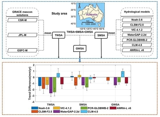
2.1. Study Area
2.2. Data
2.2.1. Hydrological Models
2.2.2. GRACE Mascon Solutions
2.3. Methodology
2.3.1. Composition of Total Terrestrial Water Storage
2.3.2. Time Series Decomposition and Trend Estimation
2.3.3. Determination of Reference Values
2.3.4. Evaluation Strategy
3. Results and Discussion
3.1. Comparison of Total Terrestrial Water Storage Trends Derived from GRACE Mascon Solutions
3.2. Evaluation of Different Water Storage Trends from Hydrological Models
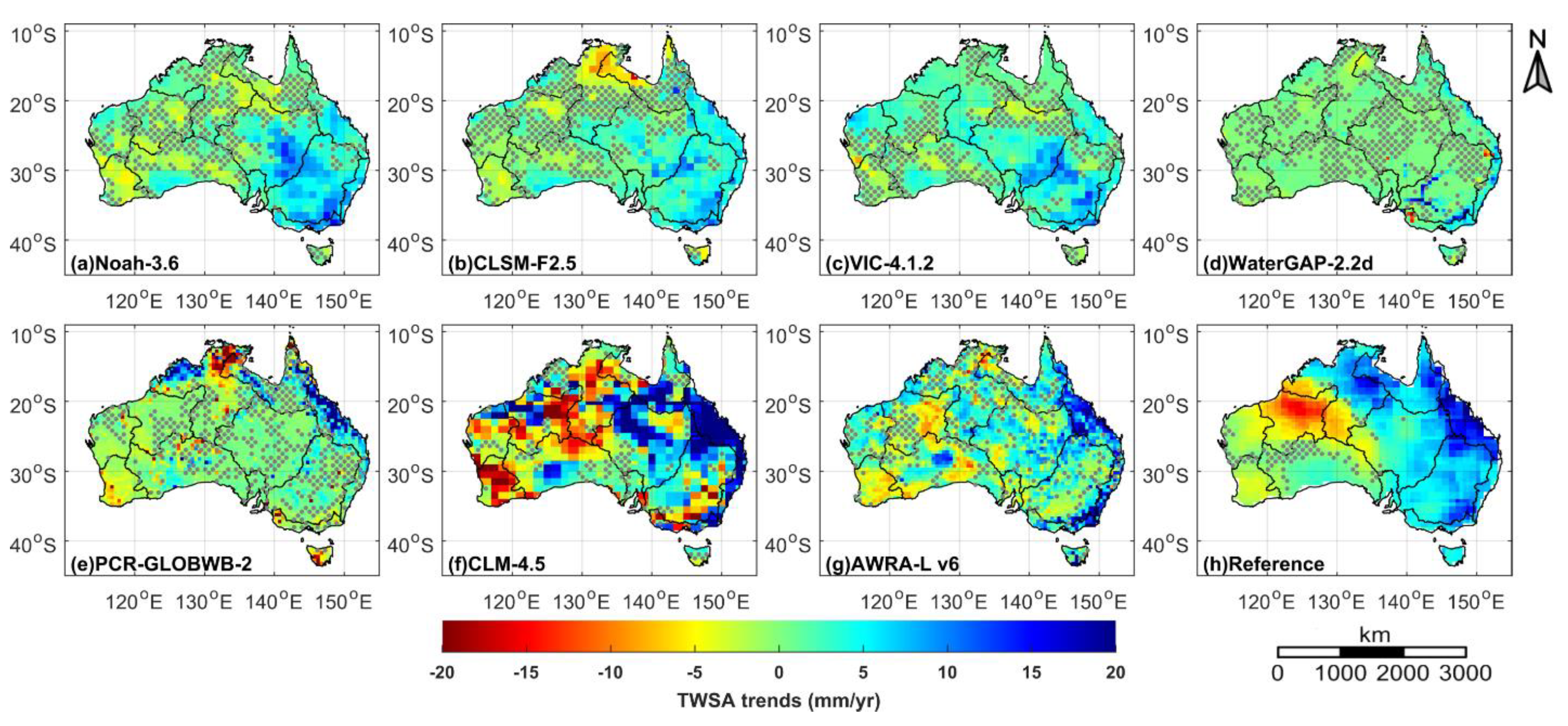
3.2.1. Total Terrestrial Water Storage Trend
3.2.2. Soil Moisture Storage Trend
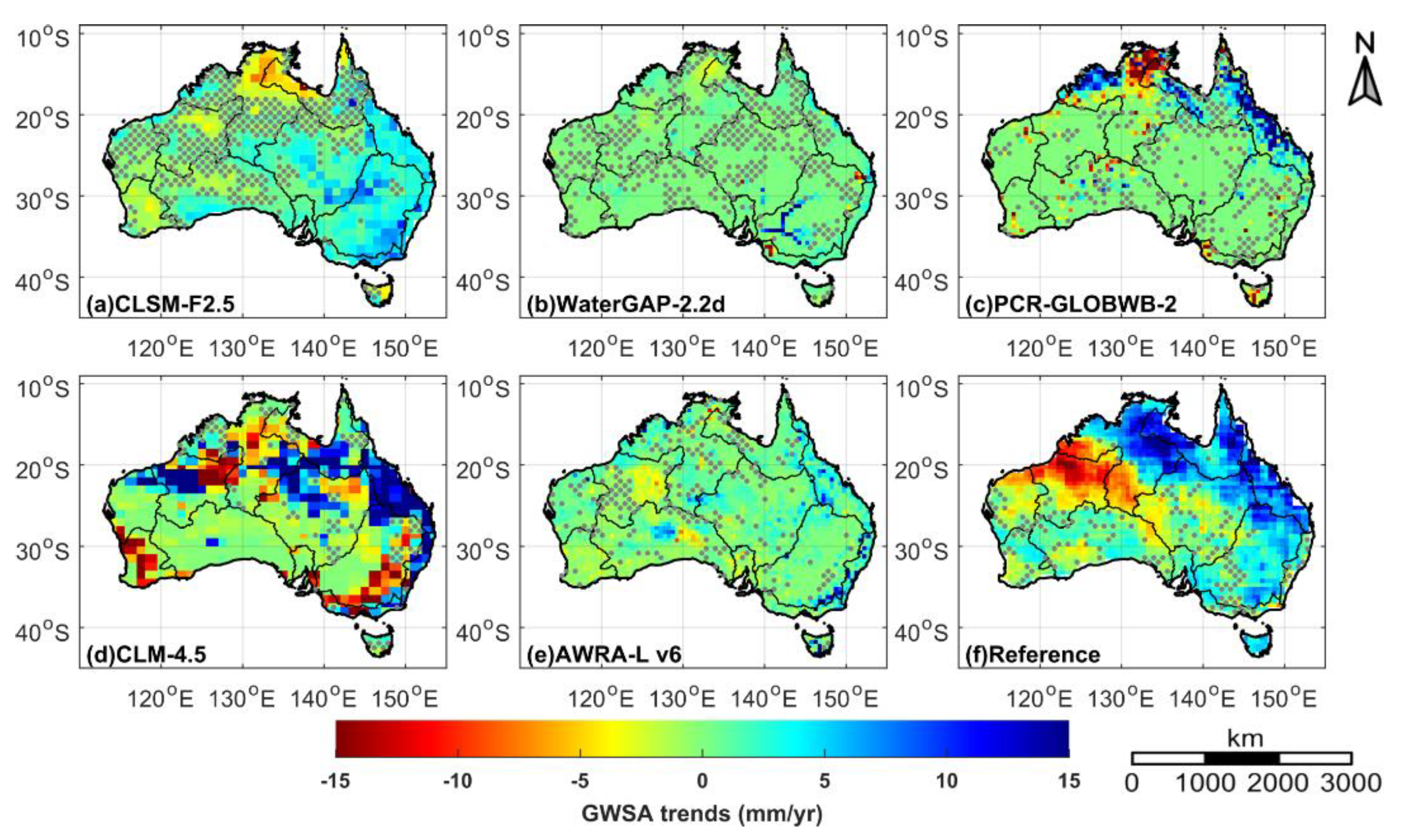
3.2.3. Groundwater Storage Trend
3.3. Influence of Model Structure on Model Uncertainty
3.4. Impact of Other Factors on Model Uncertainty
3.4.1. Climate Forcing
3.4.2. Human Water Use and Model Calibration
4. Conclusions
Supplementary Materials
Author Contributions
Funding
Acknowledgments
Conflicts of Interest
References
- Rodell, M.; Famiglietti, J.S.; Wiese, D.N.; Reager, J.T.; Beaudoing, H.K.; Landerer, F.W.; Lo, M.H. Emerging trends in global freshwater availability. Nature 2018, 557, 651–659. [Google Scholar] [CrossRef] [PubMed]
- Bierkens, M.F.P. Global hydrology 2015: State, trends, and directions. Water Resour. Res. 2015, 51, 4923–4947. [Google Scholar] [CrossRef]
- Müller Schmied, H.; Eisner, S.; Franz, D.; Wattenbach, M.; Portmann, F.T.; Flörke, M.; Döll, P. Sensitivity of simulated global-scale freshwater fluxes and storages to input data, hydrological model structure, human water use and calibration. Hydrol. Earth Syst. Sci. 2014, 18, 3511–3538. [Google Scholar] [CrossRef] [Green Version]
- Oleson, K.W.; Lawrence, D.M.; Bonan, G.B.; Flanner, M.G.; Kluzek, E.; Lawrence, P.J.; Levis, S.; Swenson, S.C.; Thornton, P.E.; Dai, M.A.; et al. Technical Description of Version 4.0 of the Community Land Model (CLM); NCAR Technical Note NCAR/TN-478+STR; National Center for Atmospheric Research: Boulder, CO, USA, 2010; 257p. [Google Scholar]
- Scanlon, B.R.; Zhang, Z.; Save, H.; Sun, A.Y.; Muller Schmied, H.; van Beek, L.P.H.; Wiese, D.N.; Wada, Y.; Long, D.; Reedy, R.C.; et al. Global models underestimate large decadal declining and rising water storage trends relative to GRACE satellite data. Proc. Natl. Acad. Sci. USA 2018, 115, E1080–E1089. [Google Scholar] [CrossRef] [PubMed] [Green Version]
- Tapley, B.D.; Bettadpur, S.; Ries, J.C.; Thompson, P.F.; Watkins, M.M. GRACE measurements of mass variability in the Earth system. Science 2004, 305, 503–505. [Google Scholar] [CrossRef] [PubMed] [Green Version]
- Leblanc, M.J.; Tregoning, P.; Ramillien, G.; Tweed, S.O.; Fakes, A. Basin-scale, integrated observations of the early 21st century multiyear drought in southeast Australia. Water Resour. Res. 2009, 45, W04408. [Google Scholar] [CrossRef]
- Chiew, F.H.S.; Young, W.J.; Cai, W.; Teng, J. Current drought and future hydroclimate projections in southeast Australia and implications for water resources management. Stoch. Environ. Res. Risk Assess. 2010, 25, 601–612. [Google Scholar] [CrossRef]
- McGrath, G.S.; Sadler, R.; Fleming, K.; Tregoning, P.; Hinz, C.; Veneklaas, E.J. Tropical cyclones and the ecohydrology of Australia’s recent continental-scale drought. Geophys. Res. Lett. 2012, 39, L03404. [Google Scholar] [CrossRef] [Green Version]
- van Dijk, A.I.J.M.; Beck, H.E.; Crosbie, R.S.; de Jeu, R.A.M.; Liu, Y.Y.; Podger, G.M.; Timbal, B.; Viney, N.R. The Millennium Drought in southeast Australia (2001-2009): Natural and human causes and implications for water resources, ecosystems, economy, and society. Water Resour. Res. 2013, 49, 1040–1057. [Google Scholar] [CrossRef]
- Zhao, M.A.G.; Velicogna, I.; Kimball, J.S. A Global Gridded Dataset of GRACE Drought Severity Index for 2002–14: Comparison with PDSI and SPEI and a Case Study of the Australia Millennium Drought. J. Hydrometeorol. 2017, 18, 2117–2129. [Google Scholar] [CrossRef] [Green Version]
- Chen, J.L.; Wilson, C.R.; Tapley, B.D.; Scanlon, B.; Güntner, A. Long-term groundwater storage change in Victoria, Australia from satellite gravity and in situ observations. Glob. Planet. Chang. 2016, 139, 56–65. [Google Scholar] [CrossRef] [Green Version]
- Yan, J.; Jia, S.; Lv, A.; Mahmood, R.; Zhu, W. Analysis of the spatio-temporal variability of terrestrial water storage in the Great Artesian Basin, Australia. Water Sci. Technol. Water Suppl. 2017, 17, 324–341. [Google Scholar] [CrossRef]
- García-García, D.; Ummenhofer, C.C.; Zlotnicki, V. Australian water mass variations from GRACE data linked to Indo-Pacific climate variability. Remote Sens. Environ. 2011, 115, 2175–2183. [Google Scholar] [CrossRef] [Green Version]
- Fasullo, J.T.; Boening, C.; Landerer, F.W.; Nerem, R.S. Australia’s unique influence on global sea level in 2010–2011. Geophys. Res. Lett. 2013, 40, 4368–4373. [Google Scholar] [CrossRef]
- Xie, Z.; Huete, A.; Restrepo-Coupe, N.; Ma, X.; Devadas, R.; Caprarelli, G. Spatial partitioning and temporal evolution of Australia’s total water storage under extreme hydroclimatic impacts. Remote Sens. Environ. 2016, 183, 43–52. [Google Scholar] [CrossRef]
- Xie, Z.; Huete, A.; Cleverly, J.; Phinn, S.; McDonald-Madden, E.; Cao, Y.; Qin, F. Multi-climate mode interactions drive hydrological and vegetation responses to hydroclimatic extremes in Australia. Remote Sens. Environ. 2019, 231, 111270. [Google Scholar] [CrossRef]
- Vishwakarma, B.; Devaraju, B.; Sneeuw, N. What Is the Spatial Resolution of grace Satellite Products for Hydrology? Remote Sens. 2018, 10, 852. [Google Scholar] [CrossRef] [Green Version]
- Tapley, B.D.; Watkins, M.M.; Flechtner, F.; Reigber, C.; Bettadpur, S.; Rodell, M.; Sasgen, I.; Famiglietti, J.S.; Landerer, F.W.; Chambers, D.P.; et al. Contributions of GRACE to understanding climate change. Nat. Clim. Chang. 2019, 5, 358–369. [Google Scholar] [CrossRef]
- van Dijk, A.I.J.M.; Renzullo, L.J.; Rodell, M. Use of Gravity Recovery and Climate Experiment terrestrial water storage retrievals to evaluate model estimates by the Australian water resources assessment system. Water Resour. Res. 2011, 47, W11524. [Google Scholar] [CrossRef]
- Swenson, S.C.; Lawrence, D.M. A GRACE-based assessment of interannual groundwater dynamics in the Community Land Model. Water Resour. Res. 2015, 51, 8817–8833. [Google Scholar] [CrossRef]
- Tangdamrongsub, N.; Han, S.-C.; Tian, S.; Müller Schmied, H.; Sutanudjaja, E.H.; Ran, J.; Feng, W. Evaluation of Groundwater Storage Variations Estimated from GRACE Data Assimilation and State-of-the-Art Land Surface Models in Australia and the North China Plain. Remote Sens. 2018, 10, 483. [Google Scholar] [CrossRef] [Green Version]
- Scanlon, B.R.; Zhang, Z.; Rateb, A.; Sun, A.; Wiese, D.; Save, H.; Beaudoing, H.; Lo, M.H.; Müller-Schmied, H.; Döll, P.; et al. Tracking Seasonal Fluctuations in Land Water Storage Using Global Models and GRACE Satellites. Geophys. Res. Lett. 2019, 46, 5254–5264. [Google Scholar] [CrossRef]
- Xia, Y.; Mocko, D.; Huang, M.; Li, B.; Rodell, M.; Mitchell, K.E.; Cai, X.; Ek, M.B. Comparison and Assessment of Three Advanced Land Surface Models in Simulating Terrestrial Water Storage Components over the United States. J. Hydrometeorol. 2017, 18, 625–649. [Google Scholar] [CrossRef]
- Bureau of Meteorology, Australian Government. Australian Hydrological Geospatial Fabric (Geofabric). Available online: http://www.bom.gov.au/water/geofabric/inuse.shtml (accessed on 22 February 2020).
- Awange, J.L.; Sharifi, M.A.; Baur, O.; Keller, W.; Featherstone, W.E.; Kuhn, M. GRACE hydrological monitoring of Australia: Current limitations and future prospects. J. Spat. Sci. 2009, 54, 23–36. [Google Scholar] [CrossRef]
- Brown, N.J.; Tregoning, P. Quantifying GRACE data contamination effects on hydrological analysis in the Murray–Darling Basin, southeast Australia. Aust. J. Earth Sci. 2010, 57, 329–335. [Google Scholar] [CrossRef] [Green Version]
- Scanlon, B.R.; Zhang, Z.; Save, H.; Wiese, D.N.; Landerer, F.W.; Long, D.; Longuevergne, L.; Chen, J. Global evaluation of new GRACE mascon products for hydrologic applications. Water Resour. Res. 2016, 52, 9412–9429. [Google Scholar] [CrossRef]
- Gupta, S.K. Modern Hydrology and Sustainable Water Development; John Wiley & Sons: Hoboken, NJ, USA, 2011. [Google Scholar]
- Rodell, M.; Houser, P.R.; Jambor, U.; Gottschalck, J.; Mitchell, K.; Meng, C.J.; Arsenault, K.; Cosgrove, B.; Radakovich, J.; Bosilovich, M.; et al. The Global Land Data Assimilation System. Bull. Am. Meteorol. Soc. 2004, 85, 381–394. [Google Scholar] [CrossRef] [Green Version]
- Sutanudjaja, E.H.; van Beek, R.; Wanders, N.; Wada, Y.; Bosmans, J.H.C.; Drost, N.; van der Ent, R.J.; de Graaf, I.E.M.; Hoch, J.M.; de Jong, K.; et al. PCR-GLOBWB 2: A 5 arcmin thinsp;arcmin global hydrological and water resources model. Geosci. Model Dev. 2018, 11, 2429–2453. [Google Scholar] [CrossRef] [Green Version]
- Oleson, K.W.; Lawrence, D.M.; Bonan, G.B.; Drewniak, B.; Huang, M.; Koven, C.D.; Levis, S.; Li, F.; Riley, W.J.; Subin, Z.M.; et al. Technical Description of Version 4.5 of the Community Land Model (CLM) NCAR Technical Note NCAR/TNG 503+STR; National Center for Atmospheric Research: Boulder, CO, USA, 2013; p. 420. [Google Scholar]
- Frost, A.J.; Ramchurn, A.; Smith, A. The Australian Landscape Water Balance Model. (AWRA-L v6). Technical Description of the Australian Water Resources Assessment Landscape Model, 6th ed.; Technical Report; The Bureau of Meteorology: Melbourne, Australia, 2018.
- NASA Land Data Assimilation System. GLDAS Specifications. Available online: https://ldas.gsfc.nasa.gov/sites/default/files/ldas/gldas/SOILS/GLDASp5_vicsoildp_10d.nc4 (accessed on 22 February 2020).
- Chen, J.L.; Wilson, C.R.; Tapley, B.D.; Grand, S. GRACE detects coseismic and postseismic deformation from the Sumatra-Andaman earthquake. Geophys. Res. Lett. 2007, 34. [Google Scholar] [CrossRef] [Green Version]
- van Dam, T.; Wahr, J.; Lavallée, D. A comparison of annual vertical crustal displacements from GPS and Gravity Recovery and Climate Experiment (GRACE) over Europe. J. Geophys. Res. 2007, 112. [Google Scholar] [CrossRef] [Green Version]
- Ivins, E.R.; Watkins, M.M.; Yuan, D.-N.; Dietrich, R.; Casassa, G.; Rülke, A. On-land ice loss and glacial isostatic adjustment at the Drake Passage: 2003–2009. J. Geophys. Res. 2011, 116. [Google Scholar] [CrossRef]
- Chambers, D.P.; Cazenave, A.; Champollion, N.; Dieng, H.; Llovel, W.; Forsberg, R.; von Schuckmann, K.; Wada, Y. Evaluation of the Global Mean Sea Level Budget between 1993 and 2014. Surv. Geophys. 2016, 38, 309–327. [Google Scholar] [CrossRef]
- Rieser, D.; Kuhn, M.; Pail, R.; Anjasmara, I.M.; Awange, J. Relation between GRACE-derived surface mass variations and precipitation over Australia. Aust. J. Earth Sci. 2010, 57, 887–900. [Google Scholar] [CrossRef]
- Tregoning, P.; McClusky, S.; Van Dijk, A.I.J.M.; Crosbie, R.S.; Peña-Arancibia, J.L. Assessment of GRACE Satellites for Groundwater Estimation in Australia; Waterlines report; National Water Commission: Canberra, Australia, 2012; p. 82. [Google Scholar]
- Save, H. “CSR GRACE RL06 Mascon Solutions”, Texas Data Repository Dataverse, V1. 2019. Available online: https://dataverse.tdl.org/dataset.xhtml;jsessionid=505699c57eee01fc06638c10a1a6?persistentId=doi%3A10.18738%2FT8%2FUN91VR&version=&q=&fileTypeGroupFacet=%22Data%22&fileAccess=&fileSortField=date (accessed on 5 February 2020).
- Save, H.; Bettadpur, S.; Tapley, B.D. High-resolution CSR GRACE RL05 mascons. J. Geophys. Res. Solid Earth 2016, 121, 7547–7569. [Google Scholar] [CrossRef]
- Watkins, M.M.; Wiese, D.N.; Yuan, D.-N.; Boening, C.; Landerer, F.W. Improved methods for observing Earth’s time variable mass distribution with GRACE using spherical cap mascons. J. Geophys. Res. Solid Earth 2015, 120, 2648–2671. [Google Scholar] [CrossRef]
- Wiese, D.N.; Landerer, F.W.; Watkins, M.M. Quantifying and reducing leakage errors in the JPL RL05M GRACE mascon solution. Water Resour. Res. 2016, 52, 7490–7502. [Google Scholar] [CrossRef]
- Luthcke, S.B.; Sabaka, T.J.; Loomis, B.D.; Arendt, A.A.; McCarthy, J.J.; Camp, J. Antarctica, Greenland and Gulf of Alaska land-ice evolution from an iterated GRACE global mascon solution. J. Glaciol. 2013, 59, 613–631. [Google Scholar] [CrossRef]
- Forootan, E.; Awange, J.L.; Kusche, J.; Heck, B.; Eicker, A. Independent patterns of water mass anomalies over Australia from satellite data and models. Remote Sens. Environ. 2012, 124, 427–443. [Google Scholar] [CrossRef] [Green Version]
- Swenson, S.; Chambers, D.; Wahr, J. Estimating geocenter variations from a combination of GRACE and ocean model output. J. Geophys. Res. Solid Earth 2008, 113, B08410. [Google Scholar] [CrossRef] [Green Version]
- Wahr, J.; Molenaar, M.; Bryan, F. Time variability of the Earth’s gravity field: Hydrological and oceanic effects and their possible detection using GRACE. J. Geophys. Res. Solid Earth 1998, 103, 30205–30229. [Google Scholar] [CrossRef]
- Rodell, M.; Chao, B.F.; Au, A.Y.; Kimball, J.S.; McDonald, K.C. Global biomass variation and its geodynamic effects. Earth Interact. 2005, 9, 1–19. [Google Scholar] [CrossRef] [Green Version]
- Getirana, A.; Kumar, S.; Girotto, M.; Rodell, M. Rivers and Floodplains as Key Components of Global Terrestrial Water Storage Variability. Geophys. Res. Lett. 2017, 44, 10359–10368. [Google Scholar] [CrossRef] [Green Version]
- Wang, J.; Song, C.; Reager, J.T.; Yao, F.; Famiglietti, J.S.; Sheng, Y.; MacDonald, G.M.; Brun, F.; Schmied, H.M.; Marston, R.A.; et al. Recent global decline in endorheic basin water storages. Nat. Geosci. 2018, 11, 926–932. [Google Scholar] [CrossRef] [Green Version]
- Cleveland, R.B.; Cleveland, W.S.; McRae, J.E.; Terpenning, I. STL: A seasonal-trend decomposition procedure based on loess. J. Off. Stat. 1990, 6, 3–73. [Google Scholar]
- Humphrey, V.; Gudmundsson, L.; Seneviratne, S.I. Assessing Global Water Storage Variability from GRACE: Trends, Seasonal Cycle, Subseasonal Anomalies and Extremes. Surv. Geophys. 2016, 37, 357–395. [Google Scholar] [CrossRef] [Green Version]
- Long, D.; Pan, Y.; Zhou, J.; Chen, Y.; Hou, X.; Hong, Y.; Scanlon, B.R.; Longuevergne, L. Global analysis of spatiotemporal variability in merged total water storage changes using multiple GRACE products and global hydrological models. Remote Sens. Environ. 2017, 192, 198–216. [Google Scholar] [CrossRef]
- Mann, H.B. Nonparametric tests against trend. Econometrica 1945, 13, 245–259. [Google Scholar] [CrossRef]
- Kendall, M.G. Rand Correlation Methods; Charles Griffin: London, UK, 1975. [Google Scholar]
- Wang, F.; Shao, W.; Yu, H.; Kan, G.; He, X.; Zhang, D.; Ren, M.; Wang, G. Re-evaluation of the Power of the Mann-Kendall Test for Detecting Monotonic Trends in Hydrometeorological Time Series. Front. Earth Sci. 2020, 8, 14. [Google Scholar] [CrossRef]
- Hamed, K.H. Trend detection in hydrologic data: The Mann–Kendall trend test under the scaling hypothesis. J. Hydrol. 2008, 349, 350–363. [Google Scholar] [CrossRef]
- Sakumura, C.; Bettadpur, S.; Bruinsma, S. Ensemble prediction and intercomparison analysis of GRACE time-variable gravity field models. Geophys. Res. Lett. 2014, 41, 1389–1397. [Google Scholar] [CrossRef]
- Holgate, C.M.; De Jeu, R.A.M.; van Dijk, A.I.J.M.; Liu, Y.Y.; Renzullo, L.J.; Vinodkumar; Dharssi, I.; Parinussa, R.M.; Van Der Schalie, R.; Gevaert, A.; et al. Comparison of remotely sensed and modelled soil moisture data sets across Australia. Remote Sens. Environ. 2016, 186, 479–500. [Google Scholar] [CrossRef]
- Tian, S.; Tregoning, P.; Renzullo, L.J.; van Dijk, A.I.J.M.; Walker, J.P.; Pauwels, V.R.N.; Allgeyer, S. Improved water balance component estimates through joint assimilation of GRACE water storage and SMOS soil moisture retrievals. Water Resour. Res. 2017, 53, 1820–1840. [Google Scholar] [CrossRef]
- Kerr, Y.H.; Al-Yaari, A.; Rodriguez-Fernandez, N.; Parrens, M.; Molero, B.; Leroux, D.; Bircher, S.; Mahmoodi, A.; Mialon, A.; Richaume, P.; et al. Overview of SMOS performance in terms of global soil moisture monitoring after six years in operation. Remote Sens. Environ. 2016, 180, 40–63. [Google Scholar] [CrossRef]
- Leblanc, M.; Tweed, S.; Van Dijk, A.; Timbal, B. A review of historic and future hydrological changes in the Murray-Darling Basin. Glob. Planet. Chang. 2012, 80–81, 226–246. [Google Scholar] [CrossRef]
- Bureau of Meteorology, Australian Government. Australian Groundwater Insight. Available online: http://www.bom.gov.au/water/groundwater/insight/#/bore/density (accessed on 15 June 2020).
- Famiglietti, J.S.; Lo, M.; Ho, S.L.; Bethune, J.; Anderson, K.J.; Syed, T.H.; Swenson, S.C.; de Linage, C.R.; Rodell, M. Satellites measure recent rates of groundwater depletion in California’s Central Valley. Geophys. Res. Lett. 2011, 38, L03403. [Google Scholar] [CrossRef] [Green Version]
- Rodell, M.; Velicogna, I.; Famiglietti, J.S. Satellite-based estimates of groundwater depletion in India. Nature 2009, 460, 999–1002. [Google Scholar] [CrossRef] [PubMed] [Green Version]
- Tangdamrongsub, N.; Han, S.-C.; Decker, M.; Yeo, I.-Y.; Kim, H. On the use of the GRACE normal equation of inter-satellite tracking data for estimation of soil moisture and groundwater in Australia. Hydrol. Earth Syst. Sci. 2018, 22, 1811–1829. [Google Scholar] [CrossRef] [Green Version]
- Göttl, F.; Schmidt, M.; Seitz, F. Mass-related excitation of polar motion: An assessment of the new RL06 GRACE gravity field models. Earth Planets Space 2018, 70, 195. [Google Scholar] [CrossRef]
- Swenson, S.C.; Lawrence, D.M. Assessing a dry surface layer-based soil resistance parameterization for the Community Land Model using GRACE and FLUXNET-MTE data. J. Geophys. Res. Atmos. 2014, 119, 10299–10312. [Google Scholar] [CrossRef]
- Tregoning, P.; Lambeck, K.; Ramillien, G. GRACE estimates of sea surface height anomalies in the Gulf of Carpentaria, Australia. Earth Planet. Sci. Lett. 2008, 271, 241–244. [Google Scholar] [CrossRef]
- Bureau of Meteorology, Australian Government. Australian Groundwater Insight. Available online: http://www.bom.gov.au/water/groundwater/insight/#/gwtrend/10yeartrend/lower_2014 (accessed on 20 June 2020).
- Hu, K.X.; Awange, J.L.; Kuhn, M.; Saleem, A. Spatio-temporal groundwater variations associated with climatic and anthropogenic impacts in South-West Western Australia. Sci. Total Environ. 2019, 696, 133599. [Google Scholar] [CrossRef] [PubMed]
- Goddard Earth Sciences Data and Information Services Center (GES DISC), NASA. Available online: https://disc.gsfc.nasa.gov/datasets?keywords=GLDAS (accessed on 22 February 2020).
- Physical Oceanography Distributed Active Archive Center, Jet Propulsion Laboratory, NASA. Available online: http://grace.jpl.nasa.gov/data/get-data/jpl_global_mascons/ (accessed on 7 February 2020).
- Goddard Earth Science Research, NASA. Available online: https://earth.gsfc.nasa.gov/index.php/geo/data/grace-mascons (accessed on 10 February 2020).


| Description | Noah-3.6 | CLSM-F2.5 | VIC-4.1.2 | WaterGAP-2.2d | PCR-GLOBWB-2 | CLM-4.5 | AWRA-L v6 |
|---|---|---|---|---|---|---|---|
| Resolution (lat × lon) | 1° × 1° | 1° × 1° | 1° × 1° | 0.5° × 0.5° | 0.08° × 0.08° | 0.94° × 1.25° | 0.05° × 0.05° |
| Time span | 2000–present | 2000–present | 2000–present | 1950–2016 | 1958–2015 | 1979–2014 | 1911–present |
| SnWS | Yes | Yes | Yes | Yes | Yes | Yes | Yes |
| CWS | Yes | Yes | Yes | Yes | Yes | Yes | Yes |
| SWS | No | No | No | Yes | Yes | Yes | Yes |
| SMS | Yes | Yes | Yes | Yes | Yes | Yes | Yes |
| GWS | No | Yes | No | Yes | Yes | Yes | Yes |
| Soil layers | 4 | 1 | 3 | 1 | 2 | 10 | 3 |
| Soil thickness (m) | 2.0 | 1.0 | Variable | Variable | 1.5 | 3.8 | 6.0 |
| Climate forcing 1 | (1) | (1) | (1) | (2) | (3) | (4) | (5) |
| Human water use | No | No | No | Yes | Yes | No | No |
| Calibration | No | No | No | Yes | No | No | Yes |
| Description | CSR-M RL06 v01 | JPL-M RL06 v01 | GSFC-M v02.4 |
|---|---|---|---|
| Released/native resolution (lat × lon) 1 | 0.25° × 0.25°/1° × 1° | 0.5° × 0.5°/3° × 3° | 1° × 1°/1° × 1° |
| Solution span | April 2002–June 2017 | April 2002–June 2017 | Jan 2003–July 2016 |
| Mean removed | 2004.0–2009.999 | 2004.0–2009.999 | 2004.0–2016.0 |
| Regularization | [42] | [43,44] | [45] |
| Background static field | GGM-05C 2 | GGM-05C | GOCO-05S 3 |
| Tide model | GOT4.8 (d/o 180) 4 | FES2014b (d/o 180) 5 | GOT4.7 (d/o 90) |
| AOD 6 | ECMWF 7 + MPIOM 8 | ECMWF + MPIOM | ECMWF + MOG2D 9 |
| Degree 1 Corrections | TN-13a 10 | [47] | [47] |
| C20 11 replacement | SLR 12 (TN-11) | SLR (TN-11) | SLR (TN-07) |
| GIA 13 Correction | ICE6G-D 14 | ICE6G-D | ICE6G-D |
| Mascon Solutions | r | RMSE (cm) | NSE |
|---|---|---|---|
| CSR–JPL | 0.98 | 0.66 | 0.97 |
| CSR–GSFC | 0.95 | 1.27 | 0.88 |
| JPL–GSFC | 0.94 | 1.35 | 0.86 |
| Models | TWSA | SMSA | GWSA | ||||||
|---|---|---|---|---|---|---|---|---|---|
| r | RMSE (cm) | NSE | r | RMSE (cm) | NSE | r | RMSE (cm) | NSE | |
| Noah-3.6 | 0.90 | 1.65 | 0.77 | 0.99 | 0.48 | 0.97 | - | - | - |
| CLSM-F2.5 | 0.87 | 1.99 | 0.67 | 0.95 | 2.15 | 0.40 | 0.31 | 2.57 | −2.01 |
| VIC-4.1.2 | 0.87 | 1.88 | 0.70 | 0.98 | 0.67 | 0.94 | - | - | - |
| WaterGAP-2.2d | 0.77 | 3.09 | 0.20 | 0.66 | 2.54 | 0.17 | 0.20 | 1.65 | −0.24 |
| PCR-GLOBWB-2 | 0.81 | 2.48 | 0.48 | 0.87 | 1.76 | 0.60 | 0.62 | 1.25 | 0.28 |
| CLM-4.5 | 0.95 | 1.05 | 0.91 | 0.96 | 0.79 | 0.92 | 0.80 | 0.90 | 0.63 |
| AWRA-L v6 | 0.93 | 1.44 | 0.82 | 0.99 | 0.47 | 0.97 | 0.65 | 1.30 | 0.23 |
| Models | TWSA | SMSA | GWSA |
|---|---|---|---|
| Trends | Trends | Trends | |
| Noah-3.6 | 1.74 ± 0.46 | 1.74 ± 0.46 | - |
| CLSM-F2.5 | 1.29 ± 0.56 | 0.25 ± 0.12 | 1.04 ± 0.44 |
| VIC-4.1.2 | 1.92 ± 0.39 | 1.92 ± 0.39 | - |
| WaterGAP-2.2d | 0.56 ± 0.13 | 0.28 ± 0.06 | 0.28 ± 0.08 |
| PCR-GLOBWB-2 | 0.73 ± 0.31 | −0.05 ± 0.20 | 0.78 ± 0.14 |
| CLM-4.5 | 3.79 ± 0.52 | 1.26 ± 0.36 | 2.53 ± 0.20 |
| AWRA-L v6 | 2.02 ± 0.45 | 1.42 ± 0.36 | 0.58 ± 0.10 |
| Reference 1 | 3.15 ± 0.56 | 1.58 ± 0.48 | 1.57 ± 0.32 |
Publisher’s Note: MDPI stays neutral with regard to jurisdictional claims in published maps and institutional affiliations. |
© 2020 by the authors. Licensee MDPI, Basel, Switzerland. This article is an open access article distributed under the terms and conditions of the Creative Commons Attribution (CC BY) license (http://creativecommons.org/licenses/by/4.0/).
Share and Cite
Yang, X.; Tian, S.; Feng, W.; Ran, J.; You, W.; Jiang, Z.; Gong, X. Spatio-Temporal Evaluation of Water Storage Trends from Hydrological Models over Australia Using GRACE Mascon Solutions. Remote Sens. 2020, 12, 3578. https://doi.org/10.3390/rs12213578
Yang X, Tian S, Feng W, Ran J, You W, Jiang Z, Gong X. Spatio-Temporal Evaluation of Water Storage Trends from Hydrological Models over Australia Using GRACE Mascon Solutions. Remote Sensing. 2020; 12(21):3578. https://doi.org/10.3390/rs12213578
Chicago/Turabian StyleYang, Xinchun, Siyuan Tian, Wei Feng, Jiangjun Ran, Wei You, Zhongshan Jiang, and Xiaoying Gong. 2020. "Spatio-Temporal Evaluation of Water Storage Trends from Hydrological Models over Australia Using GRACE Mascon Solutions" Remote Sensing 12, no. 21: 3578. https://doi.org/10.3390/rs12213578