1. Introduction
Monitoring surface temperature is important for many fields of science and technology, with applications ranging from a simple inspection of electronic components to climate change analysis using sea surface temperature data (SST). Most of these applications rely on remotely sensed measurements, in which temperature is derived from surface radiation emitted in the 8–14 µm wavelengths and registered by thermal infrared (TIR) cameras [
1,
2,
3]. Since the 1970s, surface temperature can be monitored with worldwide coverage retrieving TIR data from satellite platforms, being constantly used in studies developed on a regional scale, such as hydrological modeling [
3,
4,
5], forest fire detection [
6,
7], and environmental monitoring [
8]. Within the last 20 years, the use of Lepton cameras was expanded to proximal and aerial platforms reflecting technology advances with the development of cost-effective miniaturized thermal sensors [
9,
10,
11]. Some of these cameras are low power and lightweight enough to fit onto unmanned aerial vehicles (UAVs), with potential use for small-scale remote sensing where high spatial and temporal resolution is required [
11,
12]. Thermal imagery from UAVs has offered significant advances in agricultural applications, being used for plant phenotyping [
13,
14,
15], crop water stress detection [
16,
17,
18,
19,
20,
21], evapotranspiration estimation [
22], and plant disease detection [
23].
Although the miniaturization of thermal cameras was fundamental to expand the use of TIR data, this process ultimately affected the sensitivity and accuracy of these sensors [
24]. To reduce the size and weight, miniaturized thermal cameras do not include an internal cooling system, being classified as uncooled thermal cameras for this reason. Without a cooling mechanism, the internal temperature of the camera is susceptible to change during operation, affecting the sensitivity of the microbolometers that compose the sensor (focal plane array, FPA), which changes according to the internal temperature [
25]. As a result, the temperature readings change with the FPA temperature [
26,
27], introducing errors in temperature measurements. This issue becomes more evident during UAV campaigns in which the camera may experience abrupt changes in internal temperatures due to wind and temperature drift during flight [
28]. To minimize measurement bias caused by fluctuations in the FPA temperature, thermal cameras usually perform a non-uniformity correction (NUC) after a predefined time interval or temperature change by taking an image with the shutter closed [
24,
25]. Considering that the temperature is uniform across the shutter, the offset of each microbolometer is adjusted to ensure that further images will have a harmonized and accurate response signal [
25,
29]. Because NUC is based on the assumption that the shutter temperature is equivalent to the rest of the camera interior, it is argued that it would not be valid for UAV imagery since the shutter mechanism is more susceptible to temperature drift due to the wind effect than other parts inside the camera [
28]. Moreover, it is not clear if the frequency in which NUC is applied is enough to minimize sensor drift, especially for low-cost cameras that often do not allow adjustments on the NUC rate. For this reason, it is imperative that uncooled thermal cameras undergo a proper warm-up period before data acquisition to allow a temperature stabilization of FPA even when NUC is enabled [
11,
27].
Other sources of errors that can also affect the performance of thermal cameras are target emissivity, the distance between the sensor and the target object, and atmospheric condition. While emissivity can be the main source of error when deriving temperature from TIR data [
9], it can easily be adjusted using reference values that are well-documented in the literature. On the other hand, the atmospheric attenuation of TIR radiation that affects airborne and orbital data demands more resources and might be more complex to correct [
30]. The atmospheric attenuation can cause large errors on temperature measurements [
31,
32], and is mainly affected by meteorological variables like air temperature and humidity along with the distance between the camera and target object [
30]. To correct temperature measurements, the amount of radiation attenuated by the atmosphere is estimated from radiative transfer models using meteorological data and the distance between the sensor and surface as input variables [
33,
34]. Although radiative transfer models are efficient, sometimes input data is not available and the method is often considered time-consuming [
30]. Therefore, calibration methods that present a straightforward approach and account for more than one source of error are necessary to achieve accurate measurements, especially when deriving temperature from UAV thermal surveys.
Another important aspect of TIR UAV imagery is the image processing used to generate orthomosaics. Because such thermal cameras produce low resolution and poor contrast, the detection of common features among overlapped images performed during the alignment process becomes challenging, resulting in defective orthomosaics [
22,
35,
36]. To overcome this issue, some authors propose a co-registration process based on camera positions obtained from images captured simultaneously by a second camera that offers a higher resolution (usually a red blue green (RGB) or multispectral camera) [
36,
37,
38]. In this case, the dataset from the second camera is processed first and the camera positions are then transferred to the corresponding thermal dataset, which significantly improves the alignment performance. In most cases, however, the thermal sensor is not coupled with a second camera or the simultaneous trigger is not possible, demanding alternative solutions. Moreover, the blending mode used to generate the orthomosaic can also influence the final results [
13,
22]. To assign pixel values, overlapping images with distinct viewing angles can be combined in different ways, based on the blending configuration [
39]. As a result, temperature values from the same target might change according to the blending mode. Although some studies have discussed the effects of the blending configuration on thermal data [
13,
22,
28,
40], it has not been investigated how it can affect the overall precision and accuracy of temperature readings.
Within this context, in this study, we investigated the performance of a low-cost uncooled thermal camera, based on the precision and accuracy of temperature readings. We first assessed the proximal scenario, which aimed to analyze the Lepton camera under ideal conditions using factory calibration. Moreover, we investigated the camera performance on aerial conditions based on three flight altitudes conducted at different moments along the day. To overcome alignment issues, a co-registering method was proposed, and the orthomosaics produced were then evaluated according to the blending modes tested. Finally, we tested calibration models based on the ground reference temperature, aiming to reduce the residuals of temperature readings.
2. Materials and Methods
The study was designed to analyze the performance of the low-cost radiometric thermal camera FLIR Lepton 3.5 (FLIR Systems, Inc., Wilsonville, OR, USA) in proximal and aerial conditions. As an original equipment manufacturer (OEM) sensor, FLIR Lepton 3.5 is designed to be built into a variety of electronic products (i.e., smartphones), requiring additional hardware and programming to properly work. The camera used in this study is based on an open-source project “DIY-Thermocam V2” developed by Ritter (2017), in which the Lepton module is connected to a Teensy 3.6 microcontroller (PJRC, Sherwood, OR, USA), assembled on a printed circuit board along with a lithium-polymer battery (3.7 V, 2000 mAh) and a touchscreen liquid crystal display (LCD). The Lepton sensor retail price is around $200 (USD), with the final cost of building the prototype camera (hereafter referred to as Lepton camera) about $400 (USD), which is at least three times less expensive than commercial solutions.
The Lepton camera features an uncooled VOx microbolometer FPA with a resolution of 160 × 120 pixels and a spectral range of 8–14 µm. Temperature readings are extracted from raw 14-bit images with a resolution of 0.05 °C. During the tests, the NUC was enabled with the default configuration, being performed on a three-minute interval or when the internal temperature exceeds 1.5 °C [
41].
Some other sensors were also used during the study to provide temperature reference measurements, enabling comparisons and further calibration procedures.
Table 1 details the specifications of the sensors used to acquire temperature data.
2.1. Proximal Analysis
To evaluate the precision and accuracy of temperature measurements obtained with the Lepton camera, an experiment under controlled conditions was setup using liquid water as a blackbody-like target [
3]. An FLIR E5 handheld camera (FLIR Systems, Inc., Wilsonville, OR, USA) was also used for comparison purposes, placed in a tripod along with the Lepton camera facing perpendicularly a polystyrene box at a distance of 1 m. The polystyrene box was filled with water and a thermocouple (Testo 926, Testo SE & Co. KGaA, Lenzkirch, Germany) was attached at the side of the box, with the probe positioned parallel to the water surface at a 2 mm depth to record reference temperature data.
Data collection started after a 15-min stabilization time [
28], with both cameras being trigged simultaneously to capture a single image, repeating this process after increments in target temperature of approximately 1 °C over a range from 9.1 to 52.4 °C. Each increment on the target temperature was achieved by adding hot water to the polystyrene box, taking special care on the homogenization process, and then removing the same amount of water added to maintain a constant level. Reference temperature measurements were made based on the thermocouple readings, extracted according to the registration time of each image file. The experiment was repeated three times (
n = 102) and the laboratory temperature was kept stable at 22 °C.
Temperature data of FLIR E5 was extracted using FLIR Tools software (FLIR Systems, Inc., Wilsonville, USA), configured to adjust temperature data based on an emissivity of 0.99 [
45,
46], relative humidity of 80%, air temperature of 22 °C, and target distance of 1 m. Average temperature values were obtained from each image using a box measurement tool, using pixels within the central portion of the polystyrene box. For images captured by the Lepton camera, temperature data was extracted using the open-source software ThermoVision (v. 1.10.0, Johann Henkel, Berlin, Germany). The software converts raw digital number values (DN) into temperature data based on a standard equation from the manufacturer (Equation (1)). To obtain the average temperature from each image, the same process used for FLIR E5 data was adopted, extracting the temperature values based on pixels located at the center portion of the reference target. It is worth mentioning that the boundary boxes used to extract average temperature values from each camera had equivalent dimensions, covering approximately 3200 pixels, and remained in the same position throughout the analysis since both cameras were on attached to a fixed support:
Furthermore, temperature values derived from each camera were combined with reference measurements in linear regression models, and the residuals calculated to assess the precision and accuracy of the sensors individually.
2.2. Aerial Analysis
To explore the spatial and temporal variation of surface temperature, the use of thermal data is mostly based on orthomosaics, which are obtained through photogrammetric techniques applied to aerial imagery. In comparison to proximal approaches, aerial thermal imaging is more complex, and tends to have a lower degree of precision and accuracy due to the effect of environmental conditions and factors linked to dynamic data acquisition [
24,
28,
40,
47,
48]. In addition, image processing leading up to orthomosaic obtention can also influence the results and must be taken into account. To close these gaps, aerial data acquisition was conducted in distinct scenarios, covering different weather conditions and flight altitudes, followed by tests involving orthomosaic generation, calibration strategies, and their effect on the overall precision and accuracy of the Lepton camera.
2.2.1. Data Acquisition
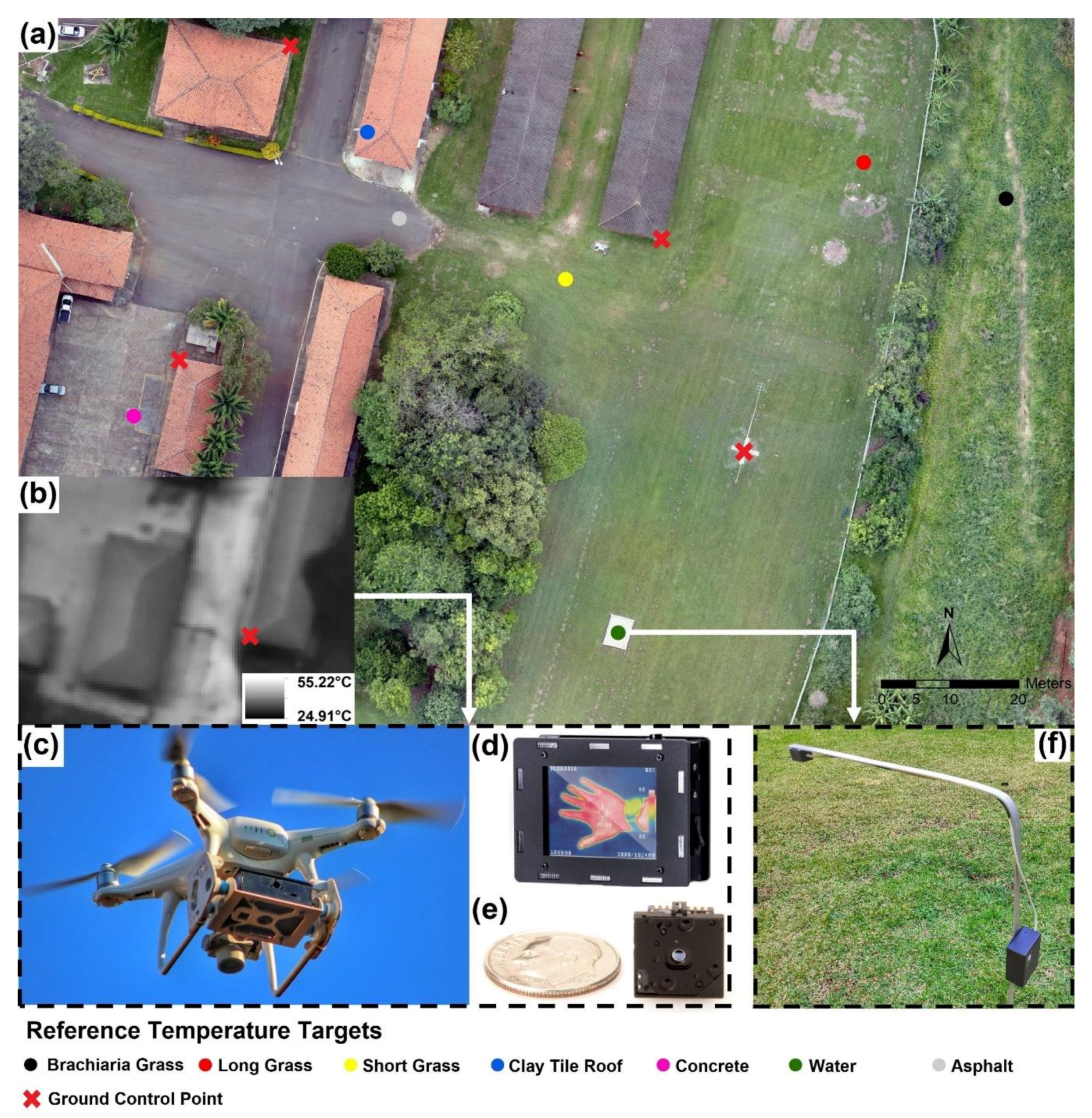
UAV missions were conducted at the Biosystems Engineering Department of Luiz de Queiroz College of Agriculture—University of São Paulo (ESALQ-USP), Piracicaba, Brazil (
Figure 1a). The Lepton camera was attached to a DJI Phantom 4 Advanced quadcopter (SZ DJI Technology Co., Shenzhen, China) using a custom-made 3-D-printed fixed support, adjusted to collect close to nadir images. Three flight plans were used for image acquisition, based on each flight altitude tested: 35, 65, and 100 m. Prior to each mission, the camera was turned on at least 15 min before the flight to ensure that camera measurements were stable [
28]. The image acquisition rate varied between 1.5 and 2 Hz among flights, corresponding to a forward overlap and side overlap of ≥80% and ≥70%, respectively, and flight speed limited to 5 m/s.
In order to capture a wider range of environmental conditions and target temperatures, the missions were performed in the early morning, close to solar noon, and at the end of the afternoon, with the three flight altitudes performed subsequently at each period, and cloudless conditions during all flights. More details regarding each mission and flight conditions are enlisted in
Table 2.
Reference measurements were obtained from seven targets distributed across the study area (
Figure 1a). These targets were selected to cover a wide range of temperatures, different types of surfaces, and materials. Additionally, we only used targets covering at least 12 m² and with enough contrast to be distinguishable in the thermal images. The temperature of the targets was monitored during each flight using MLX90614 infrared sensors (hereafter referred to as the reference sensor) (Melexis, Ypres, Belgium) (
Figure 1f). The reference sensor was installed with a nadir viewing angle 0.7 m above the target and connected to an Arduino microcontroller, recording temperature data at 5-s intervals. To ensure that reference temperature measurements were adjusted to an equivalent emissivity, the reference sensors were submitted to the protocol described in
Section 2.1, in which an empirical line calibration was developed for each device using water as a blackbody-like target [
3] (
R²val = 0.999, RMSE = 0.28 °C). Even though the emissivity among the selected targets may vary, we decided to use a standard value since determining the emissivity of targets in the field was not feasible, and because using emissivity values reported in the literature would add an extra layer of uncertainty to the analysis.
2.2.2. Flight Altitude Analysis
The performance of the Lepton camera in aerial conditions was first assessed based on the flight altitudes tested during the study. Although the accuracy of temperature readings is expected to be reduced when increasing the flight level, it is important to quantify the magnitude of these deviations and evaluate the overall precision to make sure further calibration procedures are feasible.
To ensure that temperature readings were obtained in a more realistic perspective, individual images were used during the analysis. This ensured that temperature data were obtained without any processing that could change the original values. In addition, the number of samples used to perform statistical analysis was significantly higher, improving the robustness of the results. For each mission, six images per target were manually selected from the database. The selection criteria included three images from each flight direction, with the target located on the central portion of the images to avoid the vignetting effect [
22,
28,
40].
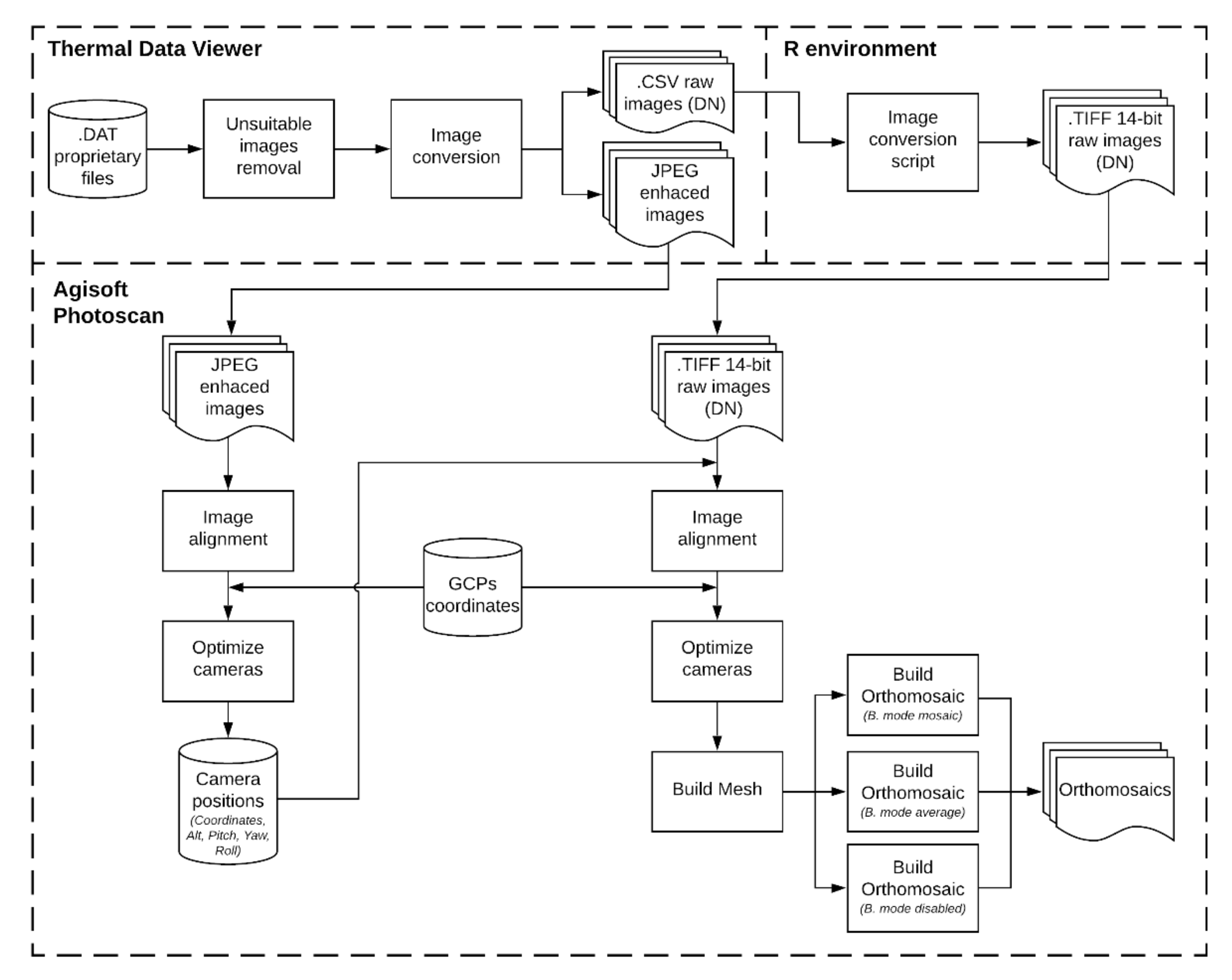
The selected images were first imported to the open-source software Thermal Data Viewer [
49], which converts in batch the proprietary files into a spreadsheet format (.CSV), and then converted into 14 bit TIFF images with DN values using R programming language [
50]. Furthermore, the TIFF images were treated individually using ArcGIS software (v. 10.2.2, ESRI Ltd., Redlands, CA, USA). The first step was to set the spatial resolution according to the GSD from
Table 2, ensuring that the pixel dimension was correct and in the metric system. Then, a circular buffer was used to extract the mean DN value, by visually locating the target and manually positioning the center point over the identified spot. Regarding the buffer size, a diameter of 1.6 m was used for all images, with average values derived from at least four pixels for missions conducted at a 100-m flying altitude, and a minimum of 11 and 43 pixels for the 65- and 35-m missions, respectively. Finally, the average DN value was converted into temperature data applying the factory model (Equation (1)), and then paired with the reference temperature using the time stamp of each image file.
2.2.3. Orthomosaic Generation and Blending Modes Analysis
Since the Lepton camera used in the study works independently from the UAV platform and does not produce geotagged images, additional steps were necessary prior to orthomosaic generation. This limitation is mainly caused by the inability of the camera to precisely record the time of each image acquisition and by fluctuations in the image capture rate, which makes the process of geotagging images using GNSS data from the UAV platform impractical. To solve this issue, a co-registering process was proposed and tested, in which the camera positions were estimated applying the structure from motion (SfM) algorithm to upscaled (pixel aggregation) thermal images with enhanced contrast. Through this process, the software can stitch overlapped images and generate a 3-D point cloud [
51], resulting in estimated camera positions when adding ground control points (GCPs).
To obtain the estimated camera positions for each dataset, we first excluded all images that were not within the flight plan (taking off, landing, maneuvering) along with blurry images and images with bands of dead pixels. The remaining images were then batch converted by Thermal Data Viewer into a JPEG format with an upscaled resolution and enhanced contrast. The software applies a bilinear interpolation increasing the original resolution to 632 × 466 pixels and adjusts the contrast applying adaptive gamma correction. Furthermore, the images were loaded into Agisoft Photoscan Professional (v. 1.2.6, Agisoft LLC, St. Petersburg, Russia) and image alignment was performed with the following settings: accuracy set as the highest, pair selection as generic, standard key point limit of 20,000, and tie point limit of 1000. If images were not aligned in the first attempt, these images were manually selected along with overlapped aligned images and realigned. After being aligned, five GCPs were added to the project, with coordinates previously measured with an RTK GNSS receiver (Topcon GR-3, 1 cm accuracy, Topcon Corporation, Tokyo, Japan). As GCPs targets, we used the roof corners’ edge of buildings, which produced temperatures different enough from the surrounding targets to be distinguishable in thermal images. To reach the roof of the buildings, the GNSS receiver was attached to a telescopic pole, positioning the antenna right beside the roof corner. Finally, optimization of the camera alignment was performed, and the camera positions were exported.
To produce the orthomosaics of each mission, the same dataset used to estimate the camera positions was employed. However, in this case, the raw images were converted into 14 bit TIFF files, preserving the original resolution (160 × 120 pixels). This process was carried out by Thermal Data Viewer, exporting the proprietary files into a spreadsheet format (.CSV), and then converting into the TIFF format using R programming language. TIFF thermal images are composed of raw DN values and have reduced contrast, which, in addition to the low resolution of TIR sensors, affects the performance of SfM-based processing, especially if no camera positions are provided [
22,
35,
36,
52]. When the image positions obtained in the last step were added, the alignment process was significantly improved as a result of a pre-selection of overlapped images based on the coordinates of each image and the availability of the pitch-yaw-roll information. Moreover, the aforementioned GCPs were added to the project and the alignment optimization was executed, followed by the mesh generation. The final step was the orthomosaic creation, in which three orthomosaics were exported for each mission, based on the blending modes tested in the study: mosaic, average, and disabled. Other parameters available in Agisoft are the color correction, which was turned off, and the pixel size, which was adjusted to the maximum for all projects. An overview of all processing steps to obtain the orthomosaics is provided in
Figure 2.
The extraction of temperature values from the orthomosaics representing each blending mode tested was carried out in ArcGIS software. Using the coordinates measured by the RTK-GNSS receiver from each target location, a buffer with a 1.6-m diameter was created. Then, using the zonal statistics tool, the average DN value was extracted using the pixels within the buffer of each target and converted to temperature data using the factory calibration model (Equation (1)), being later compared with reference temperature readings. To provide more reliable reference measurements, the average temperature was calculated considering the time interval in which each of the targets appears on the aerial images. This was achieved by manually selecting sequences of images depicting the target, and extracting temperature values from the reference sensor in these intervals to calculate the average reference temperature of the target.
2.3. Empirical Line Calibration
2.3.1. Proximal Calibration
To develop a proximal calibration model for the Lepton camera, the images collected during the proximal analysis (
Section 2.1) were employed, with 70% used to calibrate the model (
n = 71), and the remaining 30% for validation (
n = 31), being selected to provide an equivalent range of temperature values for both steps. First, the average DN value was extracted from each image by the box measurement tool from ThermoVision software, using a fixed polygon to extract the pixel values within the central portion of the polystyrene box. The average DN values from images corresponding to the calibration step were then combined with reference temperature measurements on a linear regression model, which was later applied to convert DN data from images into temperature readings during the validation step. Furthermore, the temperature readings estimated through the linear regression model were compared with reference temperature data to evaluate the precision and accuracy of the calibration model developed.
2.3.2. Aerial Calibration
Considering the wide range of conditions over the data acquisition from aerial analysis, being performed with different flight altitudes and at different times of the day, we developed multiple calibration models with different levels of specificity. The first model tested the performance of a general calibration model, based on a single dataset combining all flight altitudes and periods of the day analyzed in the study. Moreover, we also evaluated the performance of calibration models generated for specific conditions, with individual models for each flight altitude and periods of the day. In addition, the proximal calibration model obtained in
Section 2.3.1 was also tested on aerial conditions to provide a parameter related to the atmospheric attenuation of TIR radiation.
To obtain the calibration models and properly compare the results, we first established a protocol that was used throughout the analysis. The dataset from the reference targets was separated into two groups, with four targets used for calibration (asphalt, brachiaria grass, clay tile roof, short grass) and the other three for the validation step (concrete, long grass, water) (
Figure 1a). These targets were selected to provide the widest range of temperature values possible for the calibration and validation process, and were employed for all the models tested, ensuring that the different models were calibrated and validated with equivalent datasets from the same targets to promote fair comparisons.
All the calibration models were generated using individual images without any processing, based on the datasets obtained during the flight altitude analysis (
Section 2.2.2). This way, we were able to increase the number of samples used to calibrate the models and avoided introducing any uncertainties from the orthomosaic processing, adding robustness to the method. To extract the average DN value from each image used for calibration, the same procedure described in the third paragraph of
Section 2.2.2 was used, in which a buffer with a 1.6-m diameter was manually positioned over the target location to extract the mean DN value and then paired with the reference temperature according to the timestamp of the image. Moreover, the datasets were organized accordingly and used to build the linear regression model of each strategy mentioned above.
To test the linear regression models obtained, we decided to use the orthomosaics instead of individual images, since the majority of users extract temperature data from aerial thermal images through orthomosaics. In addition, we decided to use only the orthomosaics generated by the blending mode that provided the best precision and accuracy during our tests, aiming to reproduce the best scenario to test calibration models. To calculate the average DN value from targets selected for validation, the method described in the fourth paragraph of
Section 2.2.3 was used, with raw DN data extracted from a 1.6-m circular buffer positioned over the target location based on coordinates measured by an RTK-GNSS receiver. The average DN value from each target was then converted into temperature applying the corresponding linear regression model previously obtained, and paired with reference temperature measurements calculated considering the time interval in which the target appears on the aerial images used to build the orthomosaic.
2.4. Statistical Analysis
To assess the performance of the Lepton camera, we compared the thermal temperature data with reference temperature readings, analyzing the relationship between the measurements and the residuals. The precision of the camera was evaluated using the coefficient of determination values (R²), whereas the accuracy was assessed based on the residuals analysis, represented by the mean error (ME), mean absolute error (MAE), root mean square error (RMSE), and the relative root mean square error (rRMSE). The same methodology was used to assess the performance of the calibration strategies, extracting the coefficients mentioned above from the residuals of the validation step, and calculating the R² value along with the significance level from the regression model obtained in the calibration step.
4. Discussion
Considering that factory calibration of radiometric Lepton cameras is performed based on proximal analysis, using temperature readings of a blackbody radiator in a controlled environment [
41], we first reproduced this scenario to assess the performance of the sensor under ideal conditions and compared the results with a commercial camera. Under a stable ambient temperature and target ranging from 9.1 to 52.4 °C, the Lepton camera delivered accuracy within the values reported by the manufacturer, with an MAE of 1.45 °C and RMSE = 1.08 °C. These results were better than the values reported by Osroosh et al. [
53] during tests using radiometric Lepton sensors, in which an MAE of 2.1 °C and RMSE = 2.4 °C were obtained from a blackbody calibrator in a temperature range from 0 to 70 °C, conducted at a room temperature of 23 °C without replication. The lower accuracy can be explained by the wider temperature range used during the tests but also the lack of a proper initial stabilization period required by uncooled thermal cameras to stabilize temperature readings [
11,
28,
54], which is not stated in the article. In comparison to the FLIR E5 camera, the accuracy of the Lepton camera readings was inferior, with residuals nearly double the E5 results (MAE = 0.48 °C, RMSE = 0.58 °C). Because E5 allows adjustments to perform calibration, optimizing temperature readings according to the informed air temperature, relative humidity, distance, and emissivity of the target, and thus more accurate results were expected. However, in terms of precision, the cameras yielded equivalent results, with
R² > 0.99.
The camera performance on aerial mode was tested on different flight altitudes with replications throughout the day, aiming to provide a wide range of environmental and flying conditions to the analysis. We first assessed the effect of the distance between the camera and the target, which was based on three flight altitudes: 35, 65, and 100 m, using temperature data extracted from individual images without any processing and with the reference target positioned close to the central portion of the frame to avoid the vignetting effect. According to factory calibrated temperature data, the overall precision was similar among the flight altitudes tested (
R² = 0.94–0.96). The accuracy, however, decreased with the increase in flight altitude, with a higher variation between 35 and 65 m. Since TIR radiation is attenuated by the atmosphere [
11,
31,
32], when increasing the distance between the camera from the target, less radiation will reach the sensor, resulting in lower temperature values and ultimately, weaker accuracy. This effect can be clearly observed on the overall regression models (
Figure 4), in which the slope from the regression line elevates towards higher flight altitudes, demonstrating that the factory calibration gradually becomes more inaccurate as the distance between the camera and target is increased. In order to quantify the amount of radiation attenuated due to scattering and absorption by the atmospheric, radiative transfer models, such as MODTRAN [
55,
56,
57,
58], are often employed to correct TIR temperature, deriving profiles according to the distance between the camera and target object, relative humidity, and atmospheric temperature. The correction profiles’ curves have a logarithmic shape when plotted against the distance between the camera and target [
59], explaining the higher contrast of accuracy between the 35- and 65-m missions, and are significantly affected by relative humidity in low altitudes [
11], justifying the distinct patterns of the coefficient values among regressions from missions conducted at different times of the day. Although radiative transfer models are considered efficient, implementing this calibration can become time-consuming for some users [
30] and require input meteorological data, which is often not available.
Furthermore, other sources of error must be taken into account, especially the variations of the internal camera temperature experienced during flight conditions, which changes the sensitivity of the microbolometers, causing unstable temperature readings across time [
24,
25,
29]. A key strategy to mitigate the variations of the internal camera temperature is implementing a stabilization time needed for the camera to warm up before image acquisition [
11,
28,
54], associated with non-uniformity correction (NUC) being switched on to compensate the internal temperature drift effect and provide a harmonized response signal across the FPA sensor [
24]. The contrasting results reported from mission A, in which the 35-m mission delivered the worst performance among flights conducted in the early morning, were probably caused by an insufficient stabilization time before image acquisition. Even though the same warm-up time was used for all missions, the early morning flights experienced air temperature values approximately 10 °C lower than other missions, increasing the temperature difference between the initial and stabilized condition. This effect becomes evident when analyzing the performance of subsequent missions from early morning (D and G), in which the camera’s performance was significantly improved as a result of a steadier internal temperature. To avoid this issue, we recommend adding extra time for camera stabilization before flight campaigns, especially when the range between the air and internal camera temperature is more pronounced. Another effective measure is adding extra flight lines at the beginning of the mission to allow the camera temperature to stabilize according to the air temperature and wind conditions encountered during flight [
28].
Regarding the orthomosaic generation, the method developed to estimate camera positions was fundamental to overcome the alignment issues encountered with raw images, frequently reported in studies using the SfM algorithm in the mosaicking process of thermal images [
22,
35,
36,
52]. In our study, performing the initial alignment process of raw images was even more difficult because the Lepton camera used did not record any coordinates for the images captured, and a post geo-tagging process was not feasible. The co-registration process based on enhanced contrast thermal images differs from other methods because it does not require additional images captured from a second camera (normally RGB) [
36,
37,
38], which is usually triggered simultaneously with the TIR sensor to allow the further co-registration process. As a result, the number of aligned images more than doubled and we were able to successfully align the raw images and generate the orthomosaics from eight out of nine missions. The only case we were not able to produce the orthomosaic was mission A, which experienced the aforementioned issues related to an insufficient warm-up time and dramatic changes in the temperature of target objects during the flight, which we believe affected the image alignment process. For this reason, missions from 35 m were not used during the blending modes and calibration analysis, maintaining only flight altitudes with complete replications to provide more reliable conclusions among the results.
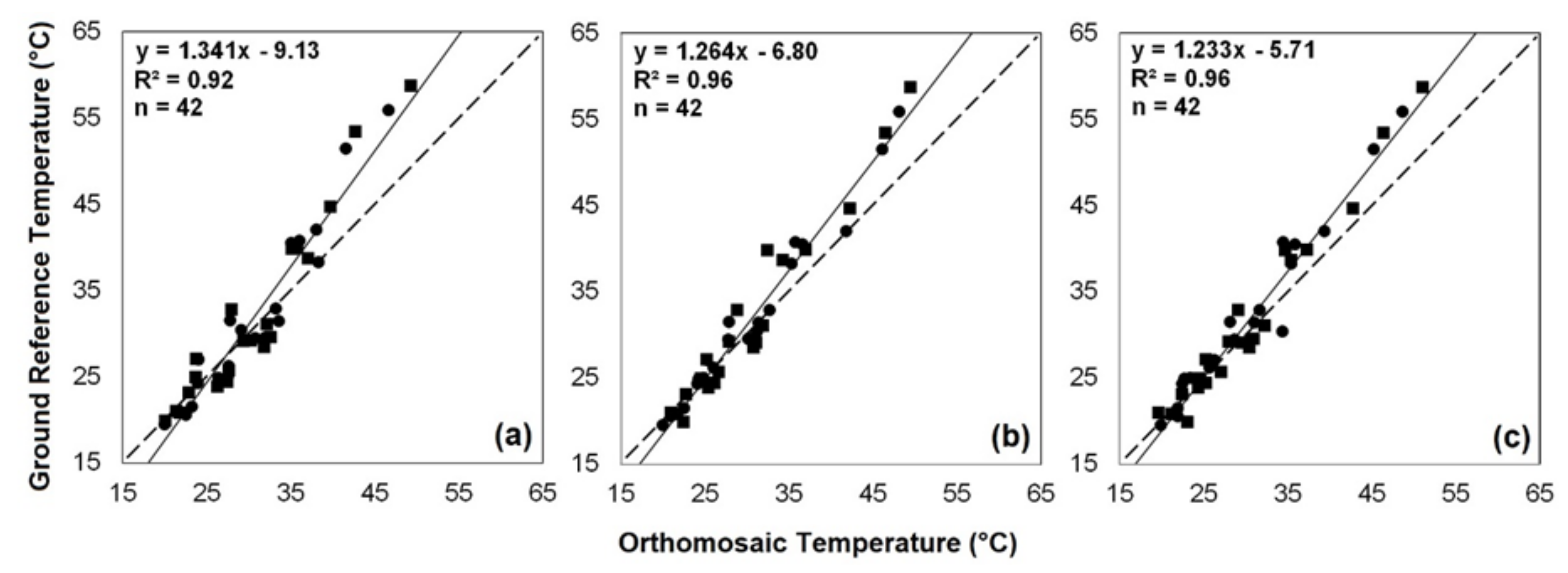
The blending modes available in Agisoft Photoscan that were tested in our study resulted in orthomosaics with significant differences in terms of precision and accuracy, with contrasting visual aspects. When the orthomosaics are generated with the blending mode disabled, each resulting pixel is extracted from a single image with the view being closest to the nadir angle [
39]. On the other hand, when activated, the blending mode merges temperature data from different images, in which the average option combines the temperature values from all images covering the target object in a simple average [
13], whereas the mosaic option applies a weighted average, with pixels closer to the nadir viewing angle being more important [
40]. The results using the disabled mode provided the best overall results, with an
R² = 0.96 and RMSE of 3.08 °C (rRMSE = 9.74%), reflecting the benefit of using only close to nadir view images to reduce the vignette effect and avoiding the extra layer of uncertainty that blending modes might introduce as reported in other studies [
22,
60]. However, the visual result from orthomosaics obtained with the blending mode disabled (
Figure 7c) can be an issue for applications aiming at the spatial distribution of TIR data, since the seamlines from the individual images used in the composition become apparent as a result of abrupt changes in temperature values from one image to another due to different viewing geometries [
13]. Results from the average blending mode were equivalent to the ones obtained with the disabled option, achieving the same overall precision (
R² = 0.96) and nearly the same accuracy, with an average RMSE of 3.14 °C (rRMSE = 9.93%). Since all overlapping images are combined in the average mode, using a wide range of camera positions and viewing angles to derive average temperature, a reduced level of accuracy is expected due to a more pronounced vignetting effect. The residuals, however, were equivalent to those obtained with the blending mode disabled, indicating that vignetting errors were not transferred to the orthomosaic generated with the average blending mode. Similar results were obtained by Hoffmann et al. [
22], in which the orthomosaic produced with the average setting delivered results that were equivalent to the same orthomosaic generated excluding all images’ edges, aiming to eliminate the vignetting effect. The final method tested was the mosaic option, which is the default blending mode in Agisoft, being constantly used to produce thermal orthomosaics [
28,
61,
62]. Although it combines features from the average and disabled mode, the performance of this method was significantly lower, with an
R² = 0.92 and RMSE of 3.93 °C (rRMSE = 12.43%), indicating that this might not be the most appropriate blending mode to produce thermal orthomosaics. Considering that this method assigns a higher weight to close to nadir view images when averaging a pixel value, the expected accuracy would be close to the values obtained with the blending mode disabled. However, it is unclear if any other factors are taken into account and how exactly the software attributes the weight of each image to calculate the average value of each pixel. Other studies that employed the mosaic blending mode to produce thermal orthomosaics achieved results within the values observed in our study, with
R² ranging from 0.70 to 0.96 and RMSE between 3.55 and 5.45 °C [
28,
61,
62].
The results using the empirical line calibration demonstrated significant improvements in the camera performance for proximal and aerial conditions. When applying a proximal calibration model, the accuracy of the Lepton camera was significantly improved in relation to the factory configuration, reducing the MAE and RMSE in 0.76 and 0.28 °C, respectively. The achieved residuals are comparable to the ones obtained with the FLIR E5 camera, which accounts for optimizations for proximal readings, and corresponds with the accuracy reported by Osroosh et al. [
53] after calibrating FLIR Lepton sensors in laboratory conditions. However, when employed in aerial conditions, the proximal calibration model yielded results equivalent to the factory calibration, with the lowest accuracy among the models tested (RMSE = 3.40 °C), indicating that proximal approaches may not be suitable for aerial imaging. To be valid, proximal calibration should account for variations in the internal camera temperature, which are mainly influenced by ambient temperature [
27,
63], and the images corrected for the attenuation of thermal radiance by the atmosphere.
On the other hand, calibration models based on the ground reference temperature consistently reduced the residuals from aerial missions, resulting in RMSE values between 1.31 and 1.94 °C. Since the models are adjusted combining TIR data with high-accuracy ground temperature, they can cover the main sources of error involved in aerial imagery, correcting the attenuation of radiation caused by the atmosphere, and reducing errors caused by variations in the camera temperature among different flights [
28]. The general model, which combines datasets from flight altitudes of 65 and 100 m, delivered the lowest residuals among the validation results, representing a reduction in MAE and RMSE values of 1.19 and 1.83 °C, respectively (MAE = 0.99 °C, RMSE = 1.31 °C). Other methods of calibration, such as the use of neural network calibration proposed by Ribeiro-Gomes et al. [
61], using sensor temperature and DN values as input variables, improved the accuracy of TIR measurements in 2.18 °C, with a final RMSE of 1.37 °C. Moreover, Mesas-Carrascosa et al. [
24] proposed a method to correct TIR temperature, removing the drift effect of microbolometer sensors based on the features used by SfM in the mosaicking process, and achieving a final accuracy within 1 °C. Using snow as the ground reference source, Pestana et al. [
64] corrected temperature derived from TIR imagery, increasing the accuracy by 1 °C. A similar approach was used by Gómez-Candón et al. [
26], in which thermal imagery was calibrated with a final accuracy of around 1 °C by using ground reference targets distributed across the flight path, deriving separate calibration models for images closest to each overpass. Furthermore, the results of specific models using individual datasets from the 65- and 100-m missions, as well as datasets dividing missions according to the time of day, provided slightly higher residuals, with RMSE values ranging from 1.32 to 1.94 °C. Even though the general model performed better in our tests, demonstrating that a more robust calibration might deliver better accuracies, the use of individual models generated from ground reference data acquired specifically for the flight campaign to be corrected ensures that any specific condition encountered will be properly covered in the calibration process, maintaining a reliable accuracy degree.


