SAR Target Classification Based on Sample Spectral Regularization

Abstract

Synthetic Aperture Radar (SAR) target classification is an important branch of SAR image interpretation. The deep learning based SAR target classification algorithms have made remarkable achievements. But the acquisition and annotation of SAR target images are time-consuming and laborious, and it is difficult to obtain sufficient training data in many cases. The insufficient training data can make deep learning based models suffering from over-fitting, which will severely limit their wide application in SAR target classification. Motivated by the above problem, this paper employs transfer-learning to transfer the prior knowledge learned from a simulated SAR dataset to a real SAR dataset. To overcome the sample restriction problem caused by the poor feature discriminability for real SAR data. A simple and effective sample spectral regularization method is proposed, which can regularize the singular values of each SAR image feature to improve the feature discriminability. Based on the proposed regularization method, we design a transfer-learning pipeline to leverage the simulated SAR data as well as acquire better feature discriminability. The experimental results indicate that the proposed method is feasible for the sample restriction problem in SAR target classification. Furthermore, the proposed method can improve the classification accuracy when relatively sufficient training data is available, and it can be plugged into any convolutional neural network (CNN) based SAR classification models.

1. Introduction

Synthetic Aperture Radar (SAR) is an important earth observation system with all-day and all-weather capability, and it has been widely used in both the military and civil fields. However, due to the complicated characteristics of SAR images, human recognition of SAR targets is difficult and inefficient. Therefore, automatic target recognition (ATR) of SAR has become a very important research direction and attracted wide attention. A standard SAR ATR process can be divided into three steps: detection, discrimination and classification. The first two steps intend to extract potential target areas and remove false alarms. The third step is to use a classifier to distinguish each SAR target. In this paper, we mainly focus on the third stage of the SAR target classification.

There are many researches on SAR target classification, which can be mainly divided into three categories: template-based methods [1,2,3], model-based methods [4,5,6,7] and machine learning based methods [8,9]. The template-based method stores a large number of SAR target templates in advance. During the inference phase, the template matching technology is used to find the most matching template for the test SAR target, then the test SAR target is classified as the category of the matched template. However, it is very difficult to obtain sufficient SAR target templates for different imaging conditions in advance, which limits the performance of the template-based SAR target classification methods. Therefore, model-based methods are proposed, which avoid the involvement of a large number of SAR target templates, but rely on the physical model for each category of the SAR target, and generate the SAR target characteristics corresponding to the model by simulation software. Besides, the statistical-model-based methods, e.g., conditionally Gaussian model [10], model different targets by statistical processes. However, the computational burden of model construction and online feature prediction is huge, which limits the performance of the model-based SAR target classification methods.

With the development of machine learning technology, machine learning based SAR target classification methods [8,9], such as AdaBoost and Support Vector Machine (SVM), have been successively proposed. The work in [11] employs iterative graph thickening to construct a two-stage SAR target classification framework. The machine learning based methods can further improve the performance of SAR ATR. However, the handcrafted features adopted in these methods [8,9,10] have limited representation capacity. Considering that the extracted features by deep convolutional neural networks have stronger representation capacity than the handcrafted features, researchers combine the deep convolutional neural network with SVM for SAT ATR [12]. Furthermore, the deep neural networks with fully connected layers as a classifier [13,14] are applied to SAR ATR. Benefiting from better deep features and end-to-end training, the deep learning based SAR ATR methods implement state-of-the-art performance.

However, the deep learning based SAR ATR methods inevitably face the challenge of sample restriction. On the one hand, the deep learning based SAR ATR methods are data-hungry. Generally, the more parameters of the deep neural networks, the more training data they require. The deep neural networks will suffer from overfitting if training with limited data example, which leads to degraded performance during the test phase. The application of deep learning based SAR ATR methods may be limited. On the other hand, the training data for SAR ATR may not be always sufficient even for the commonly used Moving and Stationary Target Acquisition and Recognition (MSTAR) dataset [15] there are only two or three hundred training images per class. More seriously, there may be only several dozens of samples for each class in practice. The reasons for sample restriction are as follows. Firstly, the valid SAR target images are not easy to collect due to some noises, e.g., speckle noise. Secondly, the annotation of the SAR target is laborious and time-consuming. Thirdly, it’s hard to collect sufficient examples for some scarce targets.

In order to solve the sample restriction problem for SAR ATR, many methods are proposed and can be divided into two categories. As shown in Figure 1a, the first category of methods is enlarging training sample sets [16,17,18,19,20,21,22,23,24,25]. To this goal, these methods resort to simulators or generative models to produce new SAR target samples. As shown in Figure 1b, the second category of methods is transfer-learning [26,27,28,29,30,31,32]. It can transfer the pre-trained knowledge from source domain to SAR target images. Specifically, in [32,33], the prior knowledge is transferred from a simulated SAR dataset to a real SAR dataset where only 10 percent of the training set is available.

Inspired by the above researches, we use transfer-learning to solve the sample restriction problem in SAR target classification. A standard pipeline is pre-training the model on a simulated SAR dataset with sufficient training data, then fine-tuning the pre-trained model with limited real SAR data. But the low feature discriminability for real SAR data may further challenge the performance, especially with the limited training data. The relation of the feature transferability and discriminability is explored in [34]. The eigenvectors of feature representations with large singular values dominate the feature transferability, while the eigenvectors with small singular values can provide extra feature discriminability. During training, the classifier relies on the salient features with large singular values as they dominate the feature representations. The features with large singular values will be strengthened and the features with small singular values will be suppressed until the model enters the saturation area of softmax activation, resulting in loss of feature discriminability from the features with small singular values.

Therefore, we propose the spectral regularization of the feature representations to improve the feature discriminability by reducing the difference between the large and small singular values and combine it with the standard transfer-learning pipeline, as shown in Figure 2. Concretely, the first proposed regularization is named sample spectral regularization (SSR), which suppresses the large singular values for the feature of each sample. The second proposed regularization named SSR${}^{†}$, which explicitly encourages more feature discriminability by narrowing the gap between the large and small singular values. Employing spectral regularization at sample-level, i.e., regularization for the feature of each training sample, can implement better performance than [34] at batch-level. Except for the sample restriction problem, the proposed spectral regularization can also improve the classification accuracy when sufficient training data is available.

Our contributions are three folds:

• We propose SSR and SSR${}^{†}$ to improve the feature discriminability by reducing the difference between the large and small singular values. The proposed SSR is at sample-level and can implement better feature discriminability than that at batch-level, which makes the classifier easier to recognize the targets of different classes.
• Based on the proposed regularization method, we propose a transfer-learning pipeline to solve the sample restriction problem in SAR target classification, which can leverage the prior knowledge from the simulated SAR data as well as has better feature discriminability.
• We further investigate the difference of various spectral regularizations. The experimental results indicate that reducing the difference between the large and small singular values at sample-level is best effective. Besides, we analyze the impact of spectral regularization on singular values.

The remainder of this paper is organized as follows. The details of the proposed method are described in Section 2. In Section 3, we conduct experiments to prove the effectiveness of the proposed method in the limited-data and sufficient-data regime and analyze the experimental results. Section 4 concludes this paper.

2. Method

In this section, we formulate the sample restriction problem for SAR target classification and address it by the proposed sample spectral regularization (SSR).

2.1. Problem Setting

The goal of this paper is to solve the sample restriction problem for SAR target classification. Let $\mathcal{S}=\left\{(x_i^s,y_i^s)\right\}$ denote a source dataset consisting of $N_s$ labeled SAR target samples from $C_s$ different classes, and $\mathcal{T}=\left\{(x_i^t,y_i^t)\right\}$ denote a target dataset consisting of $N_t$ labeled SAR target samples from $C_t$ different classes. Herein, $\mathcal{S}$ contains sufficient training samples, e.g., at least several hundreds of samples per class, $\mathcal{T}$ only contains a small number of training samples, e.g., only several dozens of samples per class. We employ a transfer-learning approach to transfer prior knowledge from a simulated SAR dataset $\mathcal{S}$ to a real SAR data set $\mathcal{T}$.

2.2. Feature Discriminability

As a key criterion to measure the representational capacity, discriminability refers to whether the model can recognize different SAR target categories successfully. Here, we revisit the relation between the feature discriminability and the singular values of the feature matrix. According to [34], the feature discriminability criterion can be formulated as follows:

$$\begin{array}{c}\hfill arg\underset{D}{max}J\left(D\right)=\frac{tr\left(D^T{S}_{inter}D\right)}{tr\left(D^T{S}_{intra}D\right)}\end{array}$$

(1)

D is a matrix for dimension reduction. $D^{\ast }$ is the optimal solution of Equation (1) and can be formulated as:

$$\begin{array}{c}\hfill D^{\ast }=arg\underset{D}{max}J\left(D\right)\end{array}$$

(2)

$S_{inter}$ and $S_{intra}$ denote the inter-class variance and intra-class variance, and can be calculated as follows:

$$\begin{array}{c}\hfill \begin{array}{c}\hfill S_{inter}=\sum _{j=1}^c{n}_j({\mu }_j-\mu ){({\mu }_j-\mu )}^T\\ \hfill S_{intra}=\sum _{j=1}^c\sum _{f\in {\mathcal{F}}_j}(f-{\mu }_j){(f-{\mu }_j)}^T\end{array}\end{array}$$

(3)

For $S_{inter}$, there are c target classes and each class has $n_j$ examples. For $S_{intra}$, there are c target classes and f is the extracted deep feature. ${\mu }_j$ denotes the center feature of j-th class. $\mu$ denotes the center feature of all classes. ${\mathcal{F}}_j$ denotes all features in j-th class. The optimal solution $D^{\ast }$ of the feature discriminability criterion can be calculated by the Singular Value Decomposition (SVD) as follows:

$$\begin{array}{c}\hfill S_{intra}^{-1}{S}_{inter}=U\Sigma V^T\end{array}$$

(4)

Thus, $D^{\ast }=U$.

The larger discriminability criterion indicates higher classification accuracy and vice versa. In the standard transfer-learning pipeline, the deep learning based classification model is pre-trained on the source dataset, then is fine-tuned on the target dataset using the pre-trained parameters as an initialization. During both phases, the model is commonly optimized by the classification loss function, e.g., the cross entropy loss. While training the model via only minimizing the classification loss cannot guarantee that the discriminability converges to the optimal solution well [34]. Therefore, we need to explicitly optimize the feature discriminability to improve the performance of the SAR target classification model training with insufficient data.

The relation between the feature discriminability and the singular values of the feature matrix is investigated in [34,35]. The eigenvectors of the feature matrix corresponding to larger singular values represent the portion of features with better transferability. The information in the eigenvectors of the feature matrix corresponding to small singular values is beneficial to improving the feature discriminability. The sharper distribution of singular values can degrade the feature discriminability. That is, strengthening the large singular values can improve the feature transferability. Strengthening the small singular values can improve the feature discriminability.

In this paper, we transfer the prior knowledge from the simulated SAR dataset $\mathcal{S}$ to real SAR dataset $\mathcal{T}$. The difference between $\mathcal{S}$ and $\mathcal{T}$ is small. Hence, the feature transferability can be guaranteed. While the discriminative information from the features corresponding to small singular values may be weakened. Consequently, we should suppress the large singular values and strengthen the small singular values to improve the feature discriminability.

2.3. Sample Spectral Regularization

A SAR target classification model consisting of a feature extractor M and a classifier $\varphi$. The feature extractor M takes a batch of SAR target images as input and outputs the extracted feature matrix $F=[f_1,f_2,...,f_b]$. b is the size of a batch. Then the extracted features are sent to the classifier $\varphi$ to output class probabilities for each sample.

A simple approach to improve the feature discriminability is suppressing the largest singular values so that the eigenvectors with small singular values can be relatively strengthened, which is named Batch Spectral Penalization (BSP) and applied in [34]. To implement BSP, the singular values of the feature matrix F are computed by singular value decomposition (SVD) as follows:

$$\begin{array}{c}\hfill F=U\Sigma V^T\end{array}$$

(5)

And $\Sigma$ can be formulated as:

$$\begin{array}{c}\hfill \Sigma =\left(\begin{array}{cccc}{\sigma }_1& 0& \cdots & 0\\ 0& {\sigma }_2& \cdots & 0\\ ⋮& ⋮& \ddots & ⋮\\ 0& 0& \cdots & {\sigma }_b\end{array}\right)\end{array}$$

(6)

Then BSP can be formulated as:

$$\begin{array}{c}\hfill BSP=\eta \sum _{i=1}^k{\sigma }_i^2\end{array}$$

(7)

where $\eta$ is a trade-off hyperparameter, ${\sigma }_i$ is the i-th singular value in the diagonal of singular value matrix $\Sigma$. [34] only suppresses the largest singular value, i.e., k is set to 1. BSP can be combined with the classification loss ${\mathcal{L}}_{cls}$ to train the model as follows:

$$\mathcal{L}={\mathcal{L}}_{cls}+BSP$$

(8)

${\mathcal{L}}_{cls}$ can be formulated as:

$$\begin{array}{c}\hfill {\mathcal{L}}_{cls}=\frac{1}{b}\sum _{i=1}^{b}l(\varphi \left(M\left(x_i\right)\right),y_i)\end{array}$$

(9)

l is the cross entropy loss.

Although BSP can improve the feature discriminability, it is conducted at batch-level and its performance can be affected by batch size, especially for the sample restriction problem where large batch size may not be available. We propose sample spectral regularization (SSR) and regularize the singular values at sample-level to bypass the above limitation of BSP. For each input SAR target example, the shape of the extracted feature f is $(W,H,C)$. W and H denote the width and height of f, and C is the number of channel. We reshape the feature f to $(W\times H,C)$ so that the singular values of f can be computed by SVD as follows:

$$\begin{array}{c}\hfill f=\stackrel{\ast }{U}\stackrel{\ast }{\Sigma }{\stackrel{\ast }{V}}^T\end{array}$$

(10)

Here, the singular value matrix $\stackrel{\ast }{\Sigma }$ is:

$$\begin{array}{c}\hfill \stackrel{\ast }{\Sigma }=\left(\begin{array}{cccc}{\stackrel{\ast }{\sigma }}_1& 0& \cdots & 0\\ 0& {\stackrel{\ast }{\sigma }}_2& \cdots & 0\\ ⋮& ⋮& \ddots & ⋮\\ 0& 0& \cdots & {\stackrel{\ast }{\sigma }}_{\tau }\end{array}\right)\end{array}$$

(11)

where $\tau =min(W\times H,C)$. Let ${\stackrel{\ast }{\sigma }}_i$ denote the set of singular values in the diagonal of singular value matrix $\stackrel{\ast }{\Sigma }$ for i-th sample within a batch, that is, ${\stackrel{\ast }{\sigma }}_i=\{{\stackrel{\ast }{\sigma }}_1,{\stackrel{\ast }{\sigma }}_2,...,{\stackrel{\ast }{\sigma }}_{\tau }\}$. Hence, ${\stackrel{\ast }{\sigma }}_{ij}$ denotes the j-th singular value in ${\stackrel{\ast }{\sigma }}_i$. The sample-level SSR can be formulated as:

$$\begin{array}{c}\hfill SSR=\eta \frac{1}{b}\sum _{i=1}^b\sum _{j=1}^k{\stackrel{\ast }{\sigma }}_{ij}^2\end{array}$$

(12)

Besides, we further improve SSR and suppress the large singular values and strengthen the small singular values by directly narrowing the gap between the largest and smallest singular values. This regularization is named SSR${}^{†}$ and can be formulated as:

$$\begin{array}{c}\hfill SS{R}^{†}=\eta \frac{1}{b}\sum _{i=1}^{b}max(max\left({\stackrel{\ast }{\sigma }}_i\right)-min\left({\stackrel{\ast }{\sigma }}_i\right),ϵ)\end{array}$$

(13)

$ϵ$ is to control the extent of the regularization constraints.

2.4. Transfer Learning with Sample Spectral Regularization

We combine the proposed SSR with the standard transfer-learning pipeline to solve the sample restriction problem of SAR target classification. Considering that generating SAR target examples by the simulator is easier than collecting real SAR target examples, we use sufficient simulated SAR data to solve the sample restriction problem, which is feasible in practice. As shown in Figure 2, the whole pipeline consists of pre-training and fine-tuning phases. During pre-training, the feature extractor M and the classifier $\varphi$ are trained on the labeled simulated SAR data. During fine-tuning, M is initialized with the pre-trained parameters and $\varphi$ is initialized randomly. Therefore, we can employ the proposed SSR during the pre-training phase to get better-initialized parameters and employ SSR during the fine-tuning phase to improve the performance of the model. The model architecture with SSR or SSR${}^{†}$ is shown in Figure 3.

Pre-train with SSR. We pre-train the model with SSR or SSR${}^{†}$ in the simulated SAR dataset $\mathcal{S}$. The loss function can be formulated as:

$$\begin{array}{c}\hfill \begin{array}{c}\hfill \mathcal{L}={\mathcal{L}}_{cls}+SSR\\ \hfill {\mathcal{L}}^{†}={\mathcal{L}}_{cls}+SS{R}^{†}\end{array}\end{array}$$

(14)

The feature extractor M is optimized by ${\mathcal{L}}_{cls}$ and the proposed regularization together. The classifier is optimized by ${\mathcal{L}}_{cls}$.

The pre-trained feature extractor $M_{pre}$ can output features with better discriminability by optimizing with the proposed SSR. This provides a good initialization for the next fine-tuning phase and makes the model converge better.

Fine-tune with SSR. We fine-tune the pre-trained model with SSR or SSR${}^{†}$ in the target SAR dataset $\mathcal{T}$. The loss function is same as in Equation (14). With a good initialization and the proposed regularization, the features from fine-tuned feature extractor $M_{ft}$ have better discriminability so that the model can yield better performance even a few training data is available.

In summary, the model is pre-trained and fine-tuned by the loss function:

$$\begin{array}{c}\hfill \mathcal{L}=\frac{1}{b}\sum _{i=1}^{b}l(\varphi \left(M\left(x_i\right)\right),y_i)+\eta \frac{1}{b}\sum _{i=1}^b\sum _{j=1}^k{\stackrel{\ast }{\sigma }}_{ij}^2\end{array}$$

(15)

or by the following loss function:

$$\begin{array}{c}\hfill {\mathcal{L}}^{†}=\frac{1}{b}\sum _{i=1}^{b}l(\varphi \left(M\left(x_i\right)\right),y_i)+\eta \frac{1}{b}\sum _{i=1}^{b}max(max\left({\stackrel{\ast }{\sigma }}_i\right)-min\left({\stackrel{\ast }{\sigma }}_i\right),ϵ)\end{array}$$

(16)

For example, the detailed process with SSR is outlined in Algorithms 1 and 2.

Algorithm 1 Pre-training process

Input: Labeled data of the simulated SAR dataset ${\mathcal{C}}_s$, feature extractor M, classifier $\varphi$, learning rate $\alpha$

Output: Pre-trained feature extractor M

1: Randomly initialize M, $\varphi$

2: while not converged do

3:     Sample b samples from ${\mathcal{C}}_s$

4:    Compute loss $\mathcal{L}=\frac{1}{b}{\sum }_{i=1}^{b}l(\varphi \left(M\left(x_i\right)\right),y_i)+\eta \frac{1}{b}{\sum }_{i=1}^b{\sum }_{j=1}^k{\stackrel{\ast }{\sigma }}_{ij}^2$

5:    Update M and $\varphi$ with gradient descent:

6:     $(M,\varphi )=(M,\varphi )-\alpha \nabla \mathcal{L}$

7: end while

Algorithm 2 Fine-tuning process

Input: Labeled data of the real SAR dataset ${\mathcal{C}}_t$, pre-trained feature extractor M, classifier $\varphi$, learning rate $\alpha$

Output: Fine-tuned feature extractor M, fine-tuned classifier $\varphi$

1: Initialized M with the pre-trained parameters, randomly initialize $\varphi$

2: while not converged do

3:     Sample b samples from ${\mathcal{C}}_t$

4:     Compute loss $\mathcal{L}=\frac{1}{b}{\sum }_{i=1}^{b}l(\varphi \left(M\left(x_i\right)\right),y_i)+\eta \frac{1}{b}{\sum }_{i=1}^b{\sum }_{j=1}^k{\stackrel{\ast }{\sigma }}_{ij}^2$

5:     Update M and $\varphi$ with gradient descent:

6:     $(M,\varphi )=(M,\varphi )-\alpha \nabla \mathcal{L}$

7: end while

2.5. An Intuitive Understanding

A convolutional neural network (CNN) based SAR target classification model commonly consists of a feature extractor and a classifier. The feature extractor is responsible for generating features that have better discriminability. Then the extracted features are used for classification. Without spectral regularization, the feature extractor M and the classifier $\varphi$ are updated with gradient descent as follows:

$$\begin{array}{c}\hfill (M,\varphi )=(M,\varphi )-\alpha \nabla {\mathcal{L}}_{cls}\end{array}$$

(17)

∇ is nabla operator.

During training, the classifier relies on the salient features with large singular values as they dominate the feature representations. As a result, the features with large singular values will be strengthened continuously and the features with small singular values will be suppressed continuously, which makes the model very confident for target classification and enter the saturation area of softmax activation, that is, the gradient magnitude $\nabla {\mathcal{L}}_{cls}$ is small. However, the features with large singular values may not always provide enough and correct information for target classification, especially with limited training data. Therefore, we need to make the model capture as much useful information as possible. The proposed spectral regularization method aims to strengthen the features with small singular values. With the proposed spectral regularization, the model is updated as follows:

$$\begin{array}{c}\hfill (M,\varphi )=(M,\varphi )-\alpha (\nabla {\mathcal{L}}_{cls}+\nabla SSR)\end{array}$$

(18)

When the model relies on the salient features with large singular values heavily, the gradient magnitude from the spectral regularization $\nabla SSR$ will be large, which can make the model leave the saturation area of softmax activation and force the classifier to use more features for classification instead of only the salient features with large singular values. Obviously, the proposed method can improve the feature discriminability and implement better SAR target classification results.

2.6. Implementation Details

We employ the same network architecture as in [33] for a fair comparison. The details of network configurations are shown in Figure 4. The feature extractor M contains four blocks. Each block consists of a convolutional layer, a batch normalization layer, a rectified linear unit (ReLU) activation function, and a $2\times 2$ max-pooling layer. The convolution stride is 1 pixel for all blocks. The output features from the feature extractor M are flattened into 1024-D vectors as the input of the classifier $\varphi$. For BSP, the extracted features are flattened into 1024-D vectors. For SSR and SSR${}^{†}$, the extracted features are reshaped into $(64,16)$ for SVD.

3. Experiment

3.1. Datasets

MSTAR. The Moving and Stationary Target Acquisition and Recognition (MSTAR) dataset is collected and released with the support of the Defense Advanced Research Projects Agency and the Air Force Research Laboratory. Figure 5 shows some SAR images and optical images for military targets in the MSTAR dataset. There are 10 military targets: T62, BTR60,ZSU234, BMP2, ZIL131, T72, BTR70, 2S1, BRDM2 and D7. The SAR data are collected by an HH-polarized X-band SAR sensor and the resolution is 0.3 m × 0.3 m. The SAR image size is $128\times 128$ pixels. The azimuth angles of target images are in the range of 0${}^{\circ }$–360${}^{\circ }$. The depression angles of target images are ${15}^{\circ }$, ${17}^{\circ }$, ${30}^{\circ }$, and ${45}^{\circ }$. The details of MSTAR are shown in

Table 1. The details of the MSTAR dataset.

Target		T72	BMP2	BTR70	BTR60	2S1	BRDM2	D7	T62	ZIL131	ZSU234
Target ID		1	2	3	4	5	6	7	8	9	10
Number	Training	232	233	233	256	299	298	299	299	299	299
	17${}^{\circ }$
Number	Test	196	196	196	195	274	274	274	273	274	274
	15${}^{\circ }$

.

The simulated SAR dataset. The simulated SAR dataset is devised by [36]. The simulated SAR images are collected using a simulation software according to the CAD models of the targets. The simulation software parameter values, e.g., material reflection coefficients and background variation, were set according to the imaging parameters of the MSTAR dataset so that the appearance of the simulated images is close to the real SAR images. There are fourteen target classes from seven types of targets due to each target type with two different CAD models. Some SAR images of the simulated SAR dataset are shown in Figure 6. The details of the simulated SAR dataset are shown in

Table 2. The details of the simulated SAR dataset.

Target	Bulldozer		Bus		Car		Humvee		Motorbike		Tank		Track
Target ID	1	2	3	4	5	6	7	8	9	10	11	12	13	14
Number	504	504	504	504	504	504	504	504	504	504	504	504	504	504

.

3.2. Training Details

During the pre-training stage, the model is trained for 400 epochs with an SGD optimizer. The learning rate is 0.001, the momentum rate is 0.9 and the weight decay is 0.0005. During the fine-tuning stage, the model is trained for 200 epochs with an SGD optimizer and the learning rate is 0.01. The hyperparameter $\eta$ is tuned through cross validation. $\eta$ is 0.01 and 0.1 for SSR and SSR${}^{†}$ respectively. $\eta$ in BSP is set to 0.001. $ϵ$ in SSR${}^{†}$ is set to zero. k in BSP and SSR is set to 1, that is, only the largest singular value is constrained.

3.3. SSR with Limited Training Data

To solve the sample restriction problem, we propose SSR and combine it with the transfer-learning pipeline. The proposed SSR suppresses large singular values and strengthens small singular values to improve the feature discriminability, which can make the deep learning based SAR classification model converge well with limited training data. In this section, we first evaluate the performance of different spectral regularization methods, then compare our best spectral regularization solution with baselines.

The performance of SSR. We evaluate the performance of BSP, SSR and SSR${}^{†}$ and the experimental results are shown in

Table 3. Test accuracies of different methods with or without spectral regularization. × denotes no any spectral regularizations. Note that the model is just trained on the limited real SAR data without the pre-training stage for ID 1, 3, 4, and 5.

ID	Pre-Training Stage				Finetuning Stage				Test Accuracy (%)
	×	BSP	SSR	SSR${}^{†}$	×	BSP	SSR	SSR${}^{†}$
1					√				75.5
2	√				√				80.2
3						√			76.1
4							√		76.6
5								√	77.8
6	√					√			82.2
7	√						√		83.4
8	√							√	84.5
9		√			√				80.7
10			√		√				81.6
11				√	√				83.2
12				√				√	88.8

. The simulated SAR dataset is used for pre-training, then we fine-tune the model using 10% of the real SAR images at a 17${}^{\circ }$ depression angle. All of the real SAR images at a 15${}^{\circ }$ depression angle are used for test. The details of the pre-training, fine-tuning and testing data are shown in Table 1 and Table 2.

Firstly, BSP, SSR and SSR${}^{†}$ are integrated into a standard training pipeline, where the model is trained from scratch (ID 3, 4, 5 in Table 3). With the three spectral regularizations, the three trained models can yield slightly higher classification accuracies than the model (ID 1 in Table 3) without spectral regularization respectively. Secondly, we initialize the models using the pre-trained parameters. then fine-tune the models with BSP, SSR and SSR${}^{†}$ respectively (ID 6, 7, 8 in Table 3). Based on the same pre-trained model, fine-tuning the model with the spectral regularizations can achieve better classification results than without spectral regularization (ID 2 in Table 3), especially SSR${}^{†}$ bringing in a 4.3% relative classification accuracy improvement. And the models with the proposed SSR and SSR${}^{†}$ significantly outperform that with BSP. Thirdly, we pre-train the models with BSP, SSR and SSR${}^{†}$ respectively, then fine-tune the models without spectral regularization to investigate how much improvements are brought by the three spectral regularizations (ID 9, 10, 11 in Table 3). Obviously, BSP, SSR and SSR${}^{†}$ can provide better-initialized parameters than pre-training without spectral regularization.

The above experimental results indicate that applying spectra regularizations to pre-training and fine-tuning can improve the final classification accuracies in the limited-data regime. SSR${}^{†}$ is the best regularization method for pre-training and fine-tuning, thus we combine SSR${}^{†}$ with the transfer-learning as our solution for the sample restriction problem (ID 12 in Table 3), which can yield the best classification accuracy of 88.8%.

Classification results Under SOC. In the limited-data regime, the model is evaluated under the standard operating condition (SOC). After pre-training with the simulated SAR images, the feature extractor M is initialized with the pre-trained parameters and the model is fine-tuned using 10% of the real SAR images at a 17${}^{\circ }$ depression angle. All of the real SAR images at a 15${}^{\circ }$ depression angle are used for test. The baseline methods are the original CNN (CNN_ORG), CNN with transfer-learning (CNN_TF) [26], CNN with parameter prediction (CNN_PP) [37], the cross-domain and cross-task method (CDCT) [32] and the probabilistic meta-learning method (PML) [33].

The experimental results are shown in

Table 4. Test accuracies with 10% of training data under SOC.

Method	CNN_ORG	CNN_TF [26]	CNN_PP [37]	CDCT [32]	PML [33]	Ours
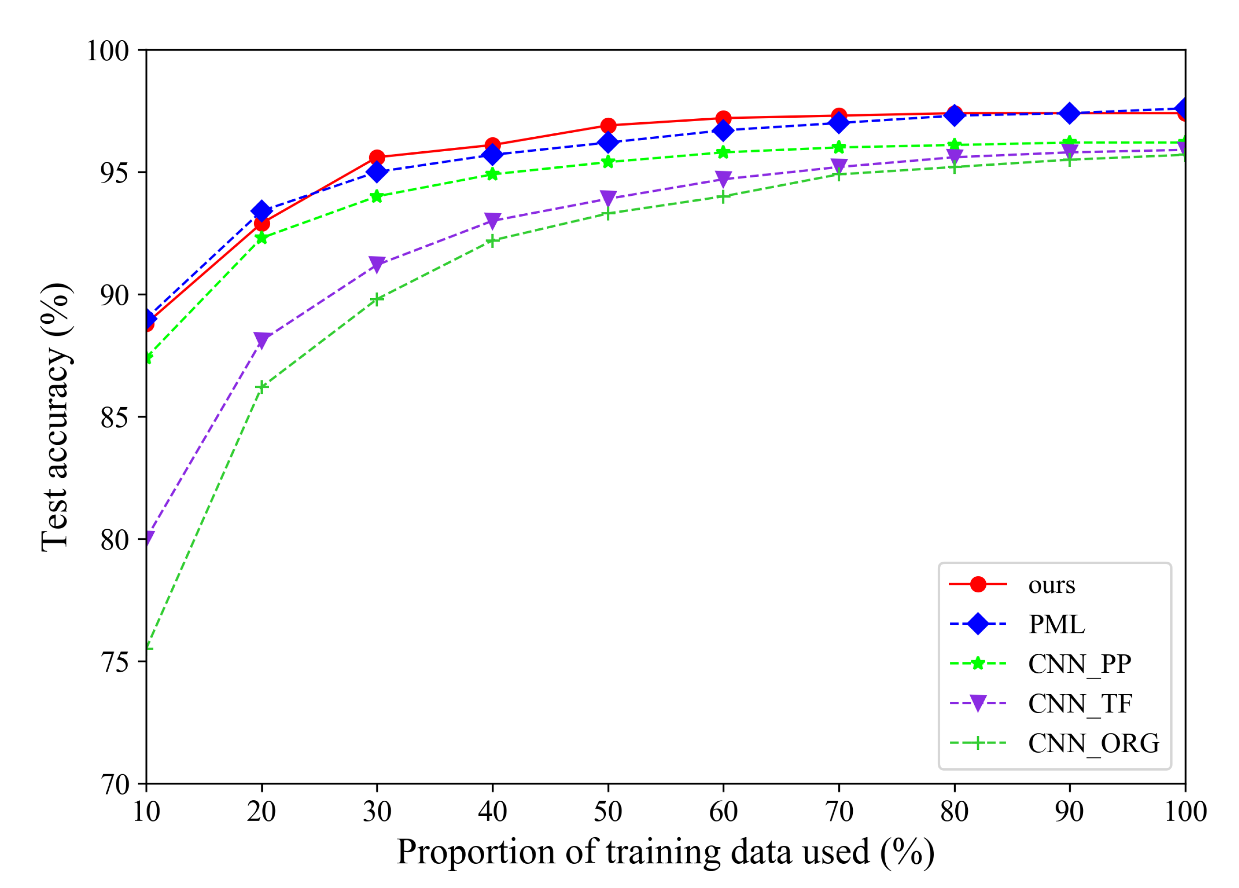
Accuracy(%)	75.5	80.2	87.4	88.9	89.0	88.8

. CNN_ORG yields the lowest classification accuracy of 75.5%. From this we can see that training the model using limited SAR data is a challenge. The standard transfer-learning can significantly improve the classification accuracy by using the prior knowledge learned from the sufficient simulated SAR images. CNN_PP, CDCT and PML achieve better classification results based on the carefully designed pipeline and model framework. In contrast, our method is very simple and effective, which achieves a comparable accuracy of 88.8% to CNN_PP, CDCT and PML.

Besides, Figure 7 illustrates the detailed classification accuracies with different proportions of training data. When increasing the proportion of training data used, the classification accuracies of all methods will become higher. Our method can achieve comparable or better performances for different proportions of training data used.

Classification results Under Depression Variations. In the limited-data regime, the model is evaluated at different depression angles. During the pre-training stage, we train the model on the simulated SAR dataset. Then, the pre-trained parameters are used to initialize the feature extractor M. We select 3 target classes from the real SAR dataset to fine-tune and test the model.

Table 5. The details of training and testing data under depression variations.

Split	Depression Angles	ZSU234	BRDM2	2S1
Training	17${}^{\circ }$	299	298	299
Test	30${}^{\circ }$	288	287	288
Test	45${}^{\circ }$	303	303	303

shows the details of the training and test data on the real SAR dataset. The model is fine-tuned on 10% of the real SAR images at a 17${}^{\circ }$ depression angle. During test time, the model is evaluated with images at 30${}^{\circ }$ and 45${}^{\circ }$ depression angles.

The experimental results are shown in

Table 6. Test accuracies with 10% of training data under depression variations.

Depression Angles	Method
	CNN_ORG	CNN_TF [26]	CDCT [32]	Ours
30${}^{\circ }$	85.6	89.2	90.3	91.0
45${}^{\circ }$	52.3	65.3	65.6	64.2

. For the 30${}^{\circ }$ depression angle, our model achieves the best classification accuracy of 91.0%. When the testing depression angle increases from 30${}^{\circ }$ to 45${}^{\circ }$, our model still yields a competitive classification result.

In summary, the above experiments prove that the proposed spectral regularization SSR${}^{†}$ is a feasible way to solve the sample restriction problem for SAR target classification. Although SSR${}^{†}$ is simple, it performs well with limited training data under SOC and depression variations.

3.4. SSR with Sufficient Training Data

In this section, we investigate how much improvement is brought by the proposed spectral regularization when fine-tuning the model with sufficient data.

Classification results Under SOC. The comparison experiments is conducted under the standard operating condition (SOC). The whole pipeline is the same as above. We pre-train the model with the simulated SAR images and initialize the feature extractor M using the pre-trained parameters. Then the model is fine-tuned using all of the real SAR images at a 17${}^{\circ }$ depression angle. We perform evaluation on the real SAR images at a 15${}^{\circ }$ depression angle. The baseline methods are CNN_ORG, CNN_TF CDCT, PML, KSR [38] and TJSR [39], CDSPP [40], KRLDP [41], MCNN [42] and MFCNN [43]. CNN_ORG and CNN_TF are selected as the simplest baselines. KSR and TJSR are two sparse representation methods, CDSPP and KRLDP are two discriminant projection methods. MCNN and MFCNN are based on convolutional neural networks (CNN).

The experimental results are shown in

Table 7. Test accuracies with full training data under SOC.

Method	Accuracy (%)
CNN_ORG	95.7
CNN_TF [26]	95.9
CNN_PP [37]	96.2
CDCT [32]	98.5
PML [33]	97.6
KSR [38]	93.6
TJSR [39]	93.4
CDSPP [40]	91.0
KRLDP [41]	95.1
MCNN [42]	98.2
MFCNN [43]	95.5
Ours	97.4

. Our method can achieve a comparable classification result to CDCT, MCNN and PML. With the proposed spectral regularization, the deep learning based feature extractor can acquire better feature discriminability, providing a 1.5 point boost in classification accuracy.

Classification results Under Depression Variations. In the sufficient-data regime, the model is evaluated at different depression angles. We pre-train the model on the simulated SAR dataset and use the pre-trained parameters as an initialization for the feature extractor M.

Three target classes from the real SAR dataset are selected to fine-tune and test the model. The details of the training and test data on the real SAR dataset are shown in Table 5. All of the real SAR images at a 17${}^{\circ }$ depression angle are used to fine-tune the model. The real SAR images at 30${}^{\circ }$ and 45${}^{\circ }$ depression angles are used for evaluation.

The experimental results are shown in

Table 8. Test accuracies with full training data under depression variations.

Method	Depression Angles
	30${}^{\circ }$	45${}^{\circ }$
CNN_ORG	91.6	60.1
CNN_TF [26]	94.0	62.5
CDCT [32]	95.8	72.5
PML [33]	96.0	79.3
KSR [38]	93.8	72.8
TJSR [39]	95.2	70.7
CDSPP [40]	92.3	77.2
KRLDP [41]	98.1	–
MCNN [42]	95.7	–
Ours	98.9	69.2

. Our model achieves the best classification accuracy of 98.9% at a 30${}^{\circ }$ depression angle, which brings in a 4.9 point boost in classification accuracy for CNN_TF. For 45${}^{\circ }$ depression angle, the classification accuracies of all methods degrade dramatically. It should be noted that the classification accuracy of CNN_TF decreases when the number of training data changes from 10% to 100%. That’s likely because the standard transfer learning cannot work well when the training images are very different from the test images [32]. While our model yields a comparable classification result to TJSR and provides a 6.7 point boost in classification accuracy for CNN_TF.

In summary, the above experiments prove that the proposed spectral regularization SSR${}^{†}$ can also promote the learning of the classification model with sufficient data. In the sufficient-data regime, cooperating with SSR${}^{†}$, the performance of CNN_TF can be significantly improved under SOC and depression variations.

3.5. SVD Analysis

In this section, we analyze the effectiveness of the proposed SSR and SSR${}^{†}$. With the pre-trained parameters as initialization, the model is fine-tuned on the real SAR images at 17${}^{\circ }$ depression angle. And the max-normalized singular values in different epochs are visualized.

Firstly, we visualize the batch-level singular values of the feature matrix $F=[f_1,f_2,...,f_b]$, which is produced from a batch of SAR image features. As shown in Figure 8, the difference between the large and small singular values is very big in the first epoch. As training progresses, the difference between the large and small singular values is decreased gradually. It is obvious that BSP makes the small singular values have more dominance than CNN_TF without spectra regularization. That is, the model with BSP has better feature discriminability. As a consequence, BSP can provide a 2.3 point boost in classification accuracy for CNN_TF.

Secondly, we visualize the singular values of the sample-level feature matrix f, which is generated by reshaping the extracted SAR image feature from $(W,H,C)$ to $(W\times H,C)$. Figure 9 shows the max-normalized sample-level singular values in different epochs. Both SSR and SSR${}^{†}$ can strengthen the small singular values to improve the feature discriminability. Obviously, SSR${}^{†}$ implements a significantly smaller difference between the large and small singular values than SSR. This is because SSR${}^{†}$ is designed to reduce the difference between the large and small singular values directly. As a consequence, SSR${}^{†}$ can provide a 4.3 point boost in classification accuracy for CNN_TF.

Although both BSP and SSR improve the feature discriminability by suppressing the largest singular values, the sample-level spectral regularization SSR performs better than the batch-level spectral regularization BSP. We think this difference comes from the level of spectral regularization. The sample-level regularization can improve the feature discriminability for each SAR image feature precisely. While the batch-level spectral regularization works for a batch of SAR image features and every image feature can affect each other. Therefore, using spectral regularization at the sample-level is more effective than batch-level (3.2% boost of SSR vs. 2.3 % of BSP).

For the original transfer-learning method, the difference between large and small singular values is always very large along with the training, and the large singular values are dominant. In contrast, for the proposed methods SSR and SSR†, the difference of large and small singular values is reduced along with the training, and the dominant position of large singular values is weakened, or small singular values are strengthened. Strengthening small singular values can make the model use more diverse discriminative information for classification and generalize well with limited training samples.

In summary, our best spectral regularization SSR${}^{†}$ directly reduces the difference of the large and small singular values at the sample-level. The effectiveness of SSR${}^{†}$ is proved by the above experiments. Applying SSR${}^{†}$ into the pre-training and fine-tuning stages can achieve better results. Besides, SSR${}^{†}$ can be plugged into any CNN based SAR target classification models to achieve performance gains no matter the training data is sufficient or not.

3.6. Noise Robustness

The small singular values strengthened by our method may contain some noise, which can degrade classification accuracy. In this paper, we combine classification loss with SSR or SSR+ and use a trade-off hyperparameter $\eta$ to balance these two terms and the classification loss is dominant. This setting can guarantee that the noise affecting discrimination will be suppressed. Therefore, the proposed method is noise-robust. This is proved by the above experiments, where our method can implement competitive classification results.

4. Conclusions

It’s difficult to train CNN based models with limited data in SAR target classification. To solve this sample restriction problem, we propose the sample spectral regularization, which can regularize the singular values of each SAR image feature to improve the feature discriminability. The proposed SSR method has been integrated into a transfer learning framework to maximize its potential performance. The experimental results indicate that the proposed regularization is a feasible approach for the sample restriction problem in SAR target classification, and conducting spectral regularization at the sample-level is better than batch-level. Besides, the proposed method can improve the classification accuracy as well when the training data is sufficient. It should be noted that our simple and effective spectral regularization can be plugged into any CNN based SAR classification models besides the implemented transfer learning framework, which is expected to benefit numerous researchers in this area.

References

1. Novak, L.M.; Owirka, G.J.; Brower, W.S.; Weaver, A.L. The automatic target-recognition system in SAIP. Linc. Lab. J. 1997, 10, 187–202. [Google Scholar]
2. Novak, L.M.; Owirka, G.J.; Brower, W.S. Performance of 10- and 20-target MSE classifiers. IEEE Trans. Aerosp. Electron. Syst. 2000, 36, 1279–1289. [Google Scholar]
3. Novak, L.M.; Halversen, S.D.; Owirka, G.J.; Hiett, M. Effects of polarization and resolution on SAR ATR. IEEE Trans. Aerosp. Electron. Syst. 1997, 33, 102–116. [Google Scholar] [CrossRef]
4. Ikeuchi, K.; Wheeler, M.D.; Yamazaki, T.; Shakunaga, T. Model-based SAR ATR system. Proc. SPIE 1996, 2757, 376–387. [Google Scholar]
5. Ross, T.D.; Bradley, J.J.; Hudson, L.J.; O’Connor, M.P. SAR ATR: So what’s the problem? An MSTAR perspective. In Algorithms for Synthetic Aperture Radar Imagery VI, Proceedings of the AEROSENSE ’99, Orlando, FL, USA, 5–9 April 1999; SPIE: Bellingham, WA USA, 1999; Volume 3721, pp. 662–672. [Google Scholar] [CrossRef]
6. Hummel, R. Model-based ATR using synthetic aperture radar. In Proceedings of the IEEE International Radar Conference, Alexandria, VA, USA, 12 May 2000; pp. 856–861. [Google Scholar]
7. Diemunsch, J.R.; Wissinger, J. Moving and stationary target acquisition and recognition (MSTAR) model-based automatic target recognition: Search technology for a robust ATR. Proc. SPIE 1998, 3370, 481–492. [Google Scholar]
8. Zhao, Q.; Principe, J.C. Support vector machines for SAR automatic target recognition. IEEE Trans. Aerosp. Electron. Syst. 2001, 37, 643–654. [Google Scholar] [CrossRef] [Green Version]
9. Sun, Y.; Liu, Z.; Todorovic, S.; Li, J. Adaptive boosting for SAR automatic target recognition. IEEE Trans. Aerosp. Electron. Syst. 2007, 43, 112–125. [Google Scholar] [CrossRef]
10. O’Sullivan, J.A.; DeVore, M.D.; Kedia, V.; Miller, M.I. SAR ATR performance using a conditionally Gaussian model. IEEE Trans. Aerosp. Electron. Syst. 2001, 37, 91–108. [Google Scholar] [CrossRef] [Green Version]
11. Srinivas, U.; Monga, V.; Raj, R.G. SAR automatic target recognition using discriminative graphical models. IEEE Trans. Aerosp. Electron. Syst. 2014, 50, 591–606. [Google Scholar] [CrossRef]
12. Wagner, S. Combination of convolutional feature extraction and support vector machines for radar ATR. In Proceedings of the 17th International Conference on Information Fusion (FUSION), Salamanca, Spain, 7–10 July 2014; pp. 1–6. [Google Scholar]
13. Morgan, D.A. Deep convolutional neural networks for ATR from SAR imagery. In Algorithms for Synthetic Aperture Radar Imagery XXII, Proceedings of the SPIE DEFENSE + SECURITY, Baltimore, MD, USA, 20–24 April 2015; International Society for Optics and Photonics: Bellingham, WA, USA, 2015; Volume 9475, p. 94750F. [Google Scholar]
14. Chen, S.; Wang, H.; Xu, F.; Jin, Y.Q. Target classification using the deep convolutional networks for SAR images. IEEE Trans. Geosci. Remote. Sens. 2016, 54, 4806–4817. [Google Scholar] [CrossRef]
15. Keydel, E.R.; Lee, S.W.; Moore, J.T. MSTAR extended operating conditions: A tutorial. Proc. SPIE 1996, 2757, 228–242. [Google Scholar]
16. Shijie, J.; Ping, W.; Peiyi, J.; Siping, H. Research on data augmentation for image classification based on convolution neural networks. In Proceedings of the 2017 Chinese Automation Congress (CAC), Jinan, China, 20–22 October 2017; pp. 4165–4170. [Google Scholar]
17. Alexander, R.; Henry R, E.; Zeshan, H.; Jared, D.; Christopher, R. Learning to Compose Domain-Specific Transformations for Data Augmentation. In Proceedings of the 31st Annual Conference on Neural Information Processing Systems (NIPS 2017), Long Beach, CA, USA, 4–9 December 2017; pp. 3236–3246. [Google Scholar]
18. Cubuk, E.D.; Zoph, B.; Mané, D.; Vasudevan, V.; Le, Q.V. AutoAugment: Learning Augmentation Strategies From Data. In Proceedings of the 2019 IEEE/CVF Conference on Computer Vision and Pattern Recognition (CVPR), Long Beach, CA, USA, 15–20 June 2019; pp. 113–123. [Google Scholar]
19. Auer, S. 3D Synthetic Aperture Radar Simulation for Interpreting Complex Urban Reflection Scenarios; Deutsche Geodätische Kommission; Verlag der Bayerischen Akademie der Wissenschaften: München, Germany, 2011. [Google Scholar]
20. Hammer, H.; Schulz, K. Coherent simulation of SAR images. In Proceedings of the SPIE Image Signal Process. Remote Sens. XV, Berlin, Germany, 31 August–3 September 2009; Volume 7477, pp. 74771G-1–74771G-9. [Google Scholar]
21. Balz, T.; Stilla, U. Hybrid GPU-Based Single- and Double-Bounce SAR Simulation. IEEE Trans. Geosci. Remote. Sens. 2009, 47, 3519–3529. [Google Scholar] [CrossRef]
22. Liu, L.; Pan, Z.; Qiu, X.; Peng, L. SAR Target Classification with CycleGAN Transferred Simulated Samples. In Proceedings of the IGARSS 2018—2018 IEEE International Geoscience and Remote Sensing Symposium, Valencia, Spain, 22–27 July 2018; pp. 4411–4414. [Google Scholar]
23. Cui, Z.; Zhang, M.; Cao, Z.; Cao, C. Image Data Augmentation for SAR Sensor via Generative Adversarial Nets. IEEE Access 2019, 7, 42255–42268. [Google Scholar] [CrossRef]
24. Cao, C.; Cao, Z.; Cui, Z. LDGAN: A Synthetic Aperture Radar Image Generation Method for Automatic Target Recognition. IEEE Trans. Geosci. Remote. Sens. 2020, 58, 3495–3508. [Google Scholar] [CrossRef]
25. Wang, K.; Zhang, G.; Leng, Y.; Leung, H. Synthetic Aperture Radar Image Generation With Deep Generative Models. IEEE Geosci. Remote. Sens. Lett. 2019, 16, 912–916. [Google Scholar] [CrossRef]
26. Malmgren-Hansen, D.; Kusk, A.; Dall, J.; Nielsen, A.A.; Engholm, R.; Skriver, H. Improving SAR Automatic Target Recognition Models With Transfer Learning From Simulated Data. IEEE Geosci. Remote. Sens. Lett. 2017, 14, 1484–1488. [Google Scholar] [CrossRef] [Green Version]
27. Zhong, C.; Mu, X.; He, X.; Wang, J.; Zhu, M. SAR Target Image Classification Based on Transfer Learning and Model Compression. IEEE Geosci. Remote. Sens. Lett. 2019, 16, 412–416. [Google Scholar] [CrossRef]
28. Rostami, M.; Kolouri, S.; Eaton, E.; Kim, K. Deep Transfer Learning for Few-Shot SAR Image Classification. Remote Sens. 2019, 11, 1374. [Google Scholar] [CrossRef] [Green Version]
29. Rostami, M.; Kolouri, S.; Eaton, E.; Kim, K. SAR Image Classification Using Few-Shot Cross-Domain Transfer Learning. In Proceedings of the 2019 IEEE/CVF Conference on Computer Vision and Pattern Recognition Workshops (CVPRW), Long Beach, CA, USA, 16–17 June 2019; pp. 907–915. [Google Scholar]
30. Huang, Z.; Pan, Z.; Lei, B. Transfer Learning with Deep Convolutional Neural Network for SAR Target Classification with Limited Labeled Data. Remote Sens. 2017, 9, 907. [Google Scholar] [CrossRef] [Green Version]
31. Huang, Z.; Pan, Z.; Lei, B. What, Where, and How to Transfer in SAR Target Recognition Based on Deep CNNs. IEEE Trans. Geosci. Remote. Sens. 2020, 58, 2324–2336. [Google Scholar] [CrossRef] [Green Version]
32. Wang, K.; Zhang, G.; Leung, H. SAR Target Recognition Based on Cross-Domain and Cross-Task Transfer Learning. IEEE Access 2019, 7, 153391–153399. [Google Scholar] [CrossRef]
33. Wang, K.; Zhang, G.; Xu, Y.; Leung, H. SAR Target Recognition Based on Probabilistic Meta-Learning. IEEE Geosci. Remote. Sens. Lett. 2020, 1–5. [Google Scholar] [CrossRef]
34. Chen, X.; Wang, S.; Long, M.; Wang, J. Transferability vs. discriminability: Batch spectral penalization for adversarial domain adaptation. In Proceedings of the International Conference on Machine Learning, Long Beach, CA, USA, 9–15 June 2019; pp. 1081–1090. [Google Scholar]
35. Chen, X.; Wang, S.; Fu, B.; Long, M.; Wang, J. Catastrophic Forgetting Meets Negative Transfer: Batch Spectral Shrinkage for Safe Transfer Learning. In Advances in Neural Information Processing Systems 32; Wallach, H., Larochelle, H., Beygelzimer, A., d’Alché-Buc, F., Fox, E., Garnett, R., Eds.; Curran Associates, Inc.: Red Hook, NY, USA, 2019; pp. 1908–1918. [Google Scholar]
36. Kusk, A.; Abulaitijiang, A.; Dall, J. Synthetic SAR Image Generation using Sensor, Terrain and Target Models. In Proceedings of the EUSAR 2016: 11th European Conference on Synthetic Aperture Radar, Hamburg, Germany, 6–9 June 2016; pp. 1–5. [Google Scholar]
37. Qiao, S.; Liu, C.; Shen, W.; Yuille, A. Few-Shot Image Recognition by Predicting Parameters from Activations. In Proceedings of the 2018 IEEE/CVF Conference on Computer Vision and Pattern Recognition, Salt Lake City, UT, USA, 18–23 June 2018; pp. 7229–7238. [Google Scholar]
38. Dong, G.; Kuang, G. SAR Target Recognition Via Sparse Representation of Monogenic Signal on Grassmann Manifolds. IEEE J. Sel. Top. Appl. Earth Obs. Remote Sens. 2016, 9, 1308–1319. [Google Scholar] [CrossRef]
39. Dong, G.; Kuang, G.; Wang, N.; Zhao, L.; Lu, J. SAR Target Recognition via Joint Sparse Representation of Monogenic Signal. IEEE J. Sel. Top. Appl. Earth Obs. Remote Sens. 2015, 8, 3316–3328. [Google Scholar] [CrossRef]
40. Liu, M.; Chen, S.; Wu, J.; Lu, F.; Wang, J.; Yang, T. Configuration Recognition via Class-Dependent Structure Preserving Projections With Application to Targets in SAR Images. IEEE J. Sel. Top. Appl. Earth Obs. Remote Sens. 2018, 11, 2134–2146. [Google Scholar] [CrossRef]
41. Yu, M.; Zhang, S.; Dong, G.; Zhao, L.; Kuang, G. Target recognition in SAR image based on robust locality discriminant projection. IET Radar Sonar Navig. 2018, 12, 1285–1293. [Google Scholar] [CrossRef]
42. Min, R.; Lan, H.; Cao, Z.; Cui, Z. A Gradually Distilled CNN for SAR Target Recognition. IEEE Access 2019, 7, 42190–42200. [Google Scholar] [CrossRef]
43. Cho, J.H.; Park, C.G. Multiple Feature Aggregation Using Convolutional Neural Networks for SAR Image-Based Automatic Target Recognition. IEEE Geosci. Remote. Sens. Lett. 2018, 15, 1882–1886. [Google Scholar] [CrossRef]
Figure 1. The pipelines of (a) enlarging training sample sets and (b) transfer-learning.
Remotesensing 12 03628 g001
Figure 2. The transfer-learning pipeline with sample spectra regularization.
Remotesensing 12 03628 g002
Figure 3. The model architecture with SSR or SSR .
Remotesensing 12 03628 g003
Figure 4. Network structure of the classification model.
Remotesensing 12 03628 g004
Figure 5. The SAR images (top) and optical images (bottom) for military targets in MSTAR dataset. The SAR images are in 17 depression angle.
Remotesensing 12 03628 g005
Figure 6. Examples of the simulated SAR dataset.
Remotesensing 12 03628 g006
Figure 7. The experimental results with different proportion of training data.
Remotesensing 12 03628 g007
Figure 8. The max-normalized batch-level singular values in different epochs.
Remotesensing 12 03628 g008
Figure 9. The max-normalized sample-level singular values in different epochs.
Remotesensing 12 03628 g009