Cloudy Region Drought Index (CRDI) Based on Long-Time-Series Cloud Optical Thickness (COT) and Vegetation Conditions Index (VCI): A Case Study in Guangdong, South Eastern China

Abstract

Widespread and long-lasting drought disasters can aggravate environmental degradation. They can lead to significant economic losses and even affect social stability. The existing drought index mostly chose arid and semi-arid regions as study areas, because cloudy weather in humid and semi-humid regions hindered the satellite in its attempts to obtain the surface reflectivity. In order to solve this problem, a cloudy region drought index (CRDI) is proposed to estimate the drought of the clouded pixels. Due to the cumulative effect of drought, the antecedent drought index (ADI) has a certain impact on the calculation of the current drought. Furthermore, cloud is the only source of natural precipitation, and it also affects the evaporation and emission process on the ground. Therefore, based on the remote sensing drought index, ADI and cloud optical thickness (COT) are used to estimate the drought of pixels with missing data due to cloud occlusion. In this paper, a case study of the cloudy Guangdong, which is located in a humid area, is presented. First, we calculated the CRDI using Moderate Resolution Imaging Spectroradiometer (MODIS) data from 2003 to 2017, and then discussed the effect of CRDI with the data from 2016 as examples. Through the analysis of the parameters of regression equation, filling efficiency, rationality of the estimated value, the continuity of CRDI and the rationality of CRDI spatial distribution results, it is concluded that CRDI can effectively estimate the drought severity of the cloud-covered pixels, and more comprehensive drought data can be obtained by using CRDI. The successful application of CRDI in Guangdong shows it is robust and flexible, suggesting high efficiency and great potential for further utilization.

1. Introduction

Drought, as a serious natural disaster, has a serious impact on social economy and people’s lives [1]. It is estimated that the economic losses caused by drought around the world are far more than for other meteorological disasters [2].

There are many ways to monitor droughts. For a single sample, we can obtain soil moisture data through a soil moisture monitoring station [3,4,5,6]. Meteorological station data can also be used to monitor drought by calculating drought index, such as from the Palmer drought severity index (PDSI), the standardized precipitation index (SPI), the surface water supply index (SWSI) and so on [7,8,9,10,11]. We can also observe the growth of single plants to determine whether they are suffering from drought [12,13,14,15], etc. The spatial continuous drought data can be obtained by interpolating the sample data. However, the point source data are usually unevenly dense, and the interpolating results are uncertain. In recent years, the method of drought monitoring based on remote sensing technology became more and more popular. It has the following advantages: data acquisition is relatively easy; data revisit rate is high; and there is better continuity in space and time. In areas with high vegetation coverage, remote sensing monitoring of soil moisture content or humidity is greatly restricted. Drought monitoring through various remote sensing vegetation indexes has achieved good application effects in vegetation coverage areas. Drought monitoring based on vegetation coverage usually uses remote sensing data to establish a corresponding drought index; for example, the vegetation conditions index (VCI), the normalized difference vegetation index (NDVI) [16,17], the normalized difference water index (NDWI) [18,19], the normalized multi-band drought index (NMDI) [20,21], the anomaly vegetation index (AVI) and the vegetation temperature condition index (VTCI) [22,23]. Among them, the calculation of VCI is simple, and it can eliminate the differences brought by terrain and other factors [24]. It has been proven that VCI can monitor drought effectively and has been widely used [24,25,26,27,28]. However, in drought monitoring based on remote sensing technology it is difficult to avoid data loss due to cloud cover, especially in a cloudy region. Therefore, how to monitor the drought of clouded pixels has become an urgent problem to be solved in the study of drought in cloudy areas.

Cloud is the only source of natural precipitation, and it also affects the evaporation and emission process on the ground. In 2004, a method of drought detection by the cloud parameter method was proposed [29]. In this method, continuous cloud-free days (CCFD), cloud-free days ratio (CFDR), continuous cloudy days (CCD) and other parameters are used. The main factor determining the accuracy of the cloud parameter method is the accuracy of cloud detection. Different cloud detection methods and different threshold values may lead to different results of final drought. Among cloud parameters, cloud optical thickness (COT) has a good correlation with precipitation and evaporation and emission process on the ground [30,31,32,33]. The introduction of COT can more effectively monitor the drought situation with cloud elements.

In view of the pixels of drought value that cannot be obtained during the monitoring period due to cloud cover, a cloudy region drought index (CRDI) inversion model based on COT and ADI was discussed. CRDI can be used to estimate the drought index of cloudy pixels. Furthermore, this model solves the problem in which the traditional remote sensing drought model is easily affected by cloud, which leads to zero value or the misjudgment of drought products. CRDI provides a possibility for more accurate real-time remote sensing drought monitoring in cloudy areas.

2. Materials and Methods

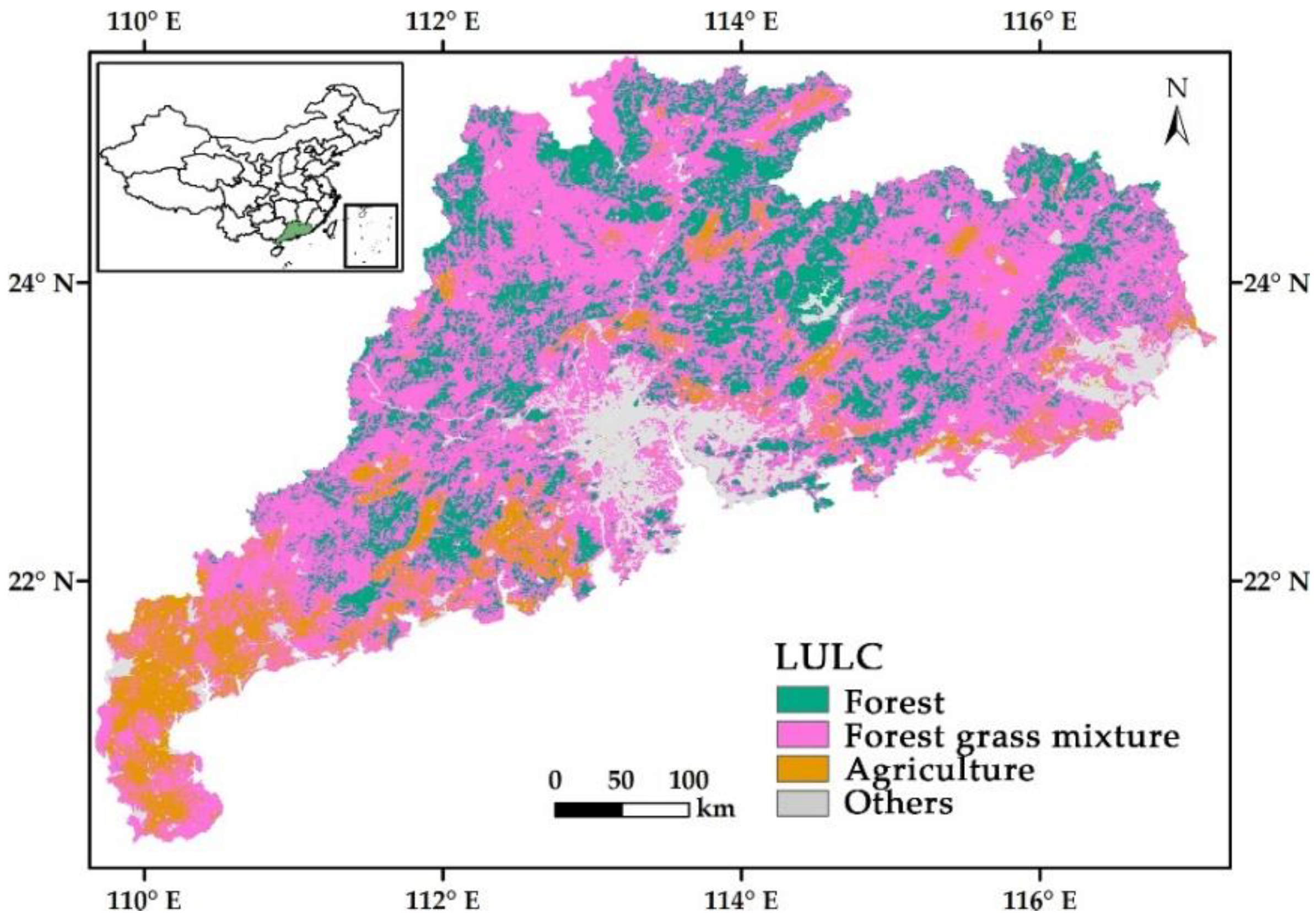
2.1. Study Area

Our study area Guangdong is located in the humid area of southern China, belonging to the East Asian monsoon climate [34]. Its annual average temperature is 19–24 °C, the annual average sunshine hours are 1745.8 h and the annual average precipitation is around 1800 mm [35]. Guangdong is mainly affected by a monsoon climate, with more precipitation, sufficient water vapor supply and more cloud cover [36]. It is also plagued by seasonal drought under the influence of multiple factors such as the monsoon, geography and geological conditions. Drought is threatening the agriculture of the whole province continuously, and it is also affecting all aspects of social life seriously. The vegetation coverage rate in Guangdong is very high, which is more than 90%, and the agricultural land coverage rate is close to 10% (Figure 1). Among them, the pixels of forest, forest grass mixture and agriculture are effective pixels.

2.2. Data Source

The Moderate Resolution Imaging Spectroradiometer (MODIS) is a sensor mounted on Aqua and Terra. It provides observation data of the earth’s surface every 1–2 days, and the minimum spatial resolution of the observation data is 250 m. MODIS data have moderate resolution, long coverage time and a short revisit period and have great potential for large-scale drought monitoring. The main data used in this paper are MODIS surface reflectance data (MOD09 and MYD09) with 250 m resolution in 8 days, COT data (MOD08 and MYD08) with 1 degree resolution in 8 days, and land use/land cover (LULC) data (MCD12Q1) with 500 m resolution.

In this paper, the MODIS surface reflectance and COT products with a period of 8 days from 2003 to 2017 are used. We decided to use 8-day data since droughts are generally persistent events with varying durations, and most of the drought events can be monitored using 8-day data. For COT data, the best value of different satellite synchronization data was selected. For the surface reflectance data, after selecting the best value, the basic drought index VCI should be calculated by using the surface reflectance values of red and near infrared bands (NIR). In addition, land use/land cover data selected in this paper are the international geosphere biosphere programme (IGBP) products that can define the surface classification of ecosystems. The research object of this paper is the area with vegetation cover. In the subsequent use of land cover data, it is necessary to integrate the original land cover data of the IGBP classification scheme (

Table 1. Classification of land data after synthesis in 2016.

Category	Proportion (%)	Category Corresponding to IGBP
Forest	21.59	broad-leaved evergreen forests, evergreen coniferous forest, deciduous broad leaved forest, deciduous coniferous forest, mixed forest, closed shrubbery, sparse shrubbery.
Forest grass mixed	58.99	forested grassland, savanna, grassland.
Agricultural	9.72	farmland, farmland and natural vegetation mosaic.
No vegetation	9.7	permanent wetland, water body, bare land, ice and snow.

). For the convenience of analysis and calculation, we resample the low-resolution COT and land use data to 250 m, so as to establish the one-to-one correspondence relationship between different data sets.

3. Methodology

A new method monitor drought in a cloudy area using ADI and COT was proposed. It included the following procedures: calculation of VCI and ADI, discussion on the correlation between VCI and ADI, establishment of regression equation and construction of a CRDI model.

3.1. Calculate VCI and ADI

NDVI is the most widely used vegetation index, which is related to vegetation coverage and mainly reflects the physiological and ecological characteristics of vegetation and also reflects the background impact of the plant canopy, such as soil, ground tide, snow, dead leaves, coarseness, etc. [37].

NDVI was first proposed by Rouse [38] based on the following equation:

$$\mathrm{NDVI}=\frac{\mathrm{NIR} - \mathrm{R}}{\mathrm{NIR} + \mathrm{R}}$$

(1)

where NIR stands for the reflectivity of near infrared band, and R stands for the reflectivity of red band. The range of NDVI is between −1 and 1, the negative value indicates that the ground is covered by clouds, water, snow, etc.; 0 indicates that there is rock or bare soil, etc.; the positive value indicates that there is vegetation coverage, and its NDVI increases with the increase of vegetation coverage.

VCI is a remote sensing index based on NDVI. It is mainly used to reflect the relative growth of vegetation. VCI was first proposed by Kogan [39] and based on the following equation:

$$\mathrm{VCI}=100\times \frac{{\mathrm{NDVI}}_{\mathrm{i}} -{ \mathrm{NDVI}}_{\min }}{{\mathrm{NDVI}}_{\max } -{ \mathrm{NDVI}}_{\min }}$$

(2)

where, i ranges from 1 to 46 and is represented for the current period in a year. NDVI_i represented the NDVI value of period i in a specific year. NDVI_max and NDVI_min represented the maximum and minimum NDVI values of period i of all years and reflect the best and worst conditions of vegetation growth, respectively. Furthermore, the difference represents the habitat of vegetation, such as soil moisture, nutrition and sunshine. The smaller the difference between NDVI_i and NDVI_min, the worse the vegetation growth in the current period [39]. The range of VCI is between 0 and 100. The smaller VCI is, the worse the vegetation condition is, and the more serious the drought is [40,41].

Due to the cumulative effect of drought, the antecedent drought has a certain impact on the current drought [30]. Antecedent drought used in this paper is obtained from VCI based on the following equation:

$${\mathrm{ADI}}_{\mathrm{j}}={\mathrm{VCI}}_{\mathrm{j}-1}$$

(3)

where j represented the current period. The minimum value of j is 2, and the maximum value of j is the length of our data. We used 15 years of data, and there are 46 issues per year, so the length of our data is 690.

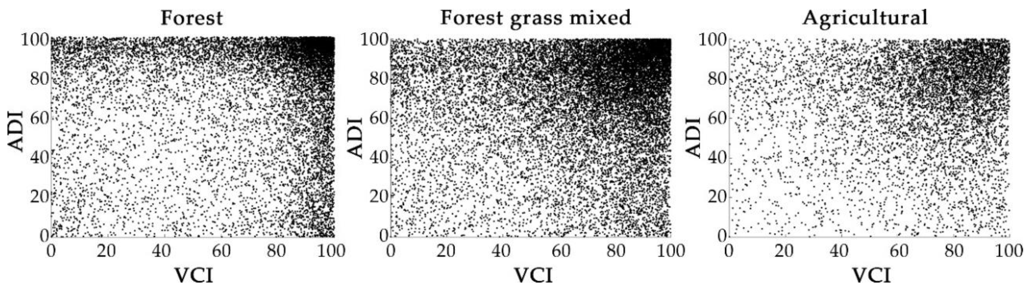
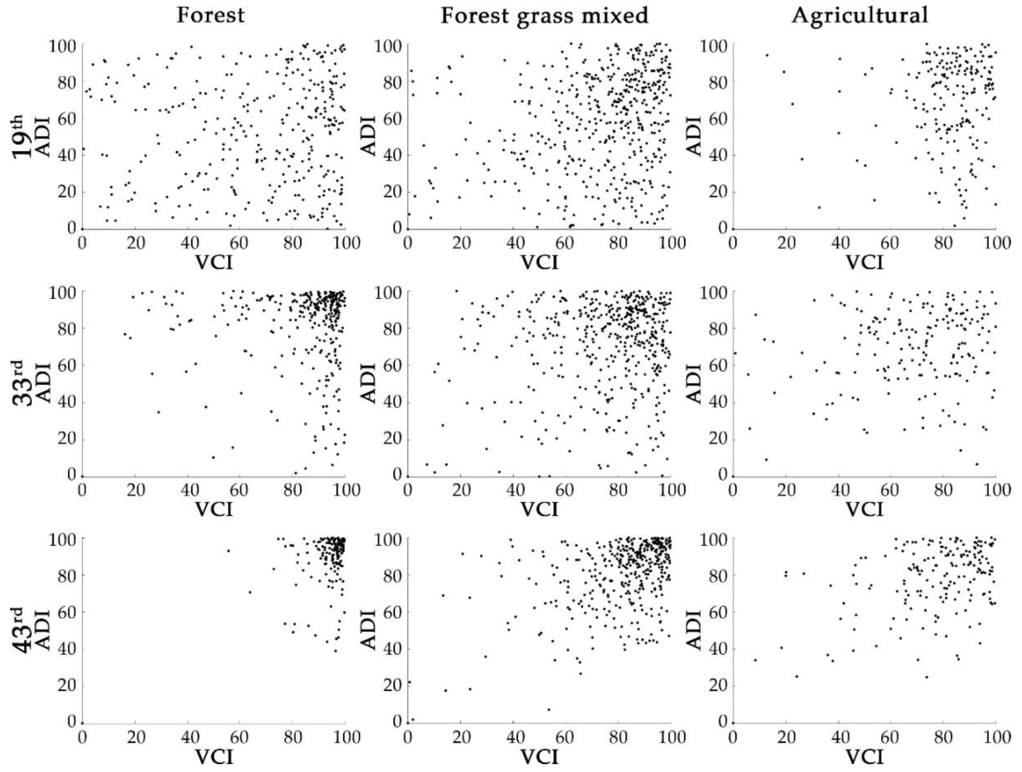
3.2. Correlation between VCI and ADI

The relationship between VCI and ADI of forest, grassland and agricultural land (Figure 2) was discussed by using the data of 2016. The points in the scatter diagram are randomly selected. It can be seen that the scattering points are basically concentrated in the upper right corner, and VCI is positively correlated with its ADI. However, for the scatter diagram of the forest, some scatter points are concentrated in the upper left and lower right. This is due to the area and species of woodland in Guangdong. Some of the points concentrated in the upper left and lower right may be related to different forest types. However, most of the points are still concentrated in the upper right corner, and there is a positive correlation on the whole. For three different land cover types, the aggregation of points in the scatter diagram are similar. However, whether the same equation can be used for different land cover types needs further investigation.

In order to explore the differences of scatter plot of different land cover types and different periods, the scatter plots of random points of the 19th, 33rd and 43rd period were selected from the 46 periods in 2016. Furthermore, period 19, 33 and 43 correspond to late-April, mid-September and early-December in 2016, respectively. The points in the scatter plot tend to be concentrated in the upper right corner, but it is obvious that the aggregation of different land cover types and different periods is different (Figure 3). Therefore, regression equations should be constructed for different land cover types and different periods.

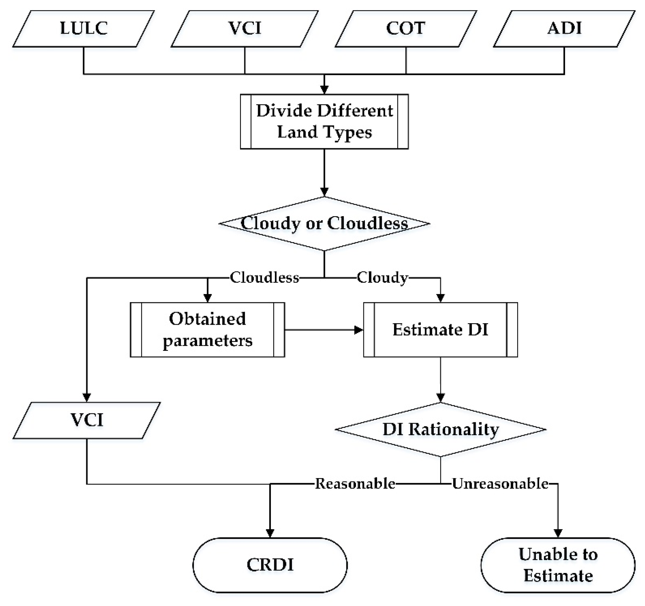
3.3. Estimation Method of Cloudy Pixel

In this paper, ADI and COT are used to estimate the drought value of the pixel in a cloudy region. Using ADI and COT to estimate the drought value of pixels in cloudy regions mainly includes the following steps. Taking the agricultural region as an example, firstly, the agricultural region in current period is extracted, and the regression equation is established according to the COT, ADI and VCI corresponding to the cloudless pixels, and then the parameters in the regression equation are obtained. Finally, according to these parameters, the drought value of cloudy pixels in agricultural region is estimated and recorded as DI. The equation for estimating DI is as follows:

$$\mathrm{DI}=\mathrm{a}+\mathrm{b}\times \mathrm{ADI}+\mathrm{c}\times \mathrm{COT}+\mathsf{\tau }$$

(4)

where, a is the constant term, b is the coefficient of ADI, c is the coefficient of COT and τ is the residual of the regression equation. Finally, it is necessary to judge whether the estimated value DI is reasonable. VCI ranges from 0 to 100, so the boundary of DI should also be within 0 and 100. When the value of DI exceeds the boundary but does not exceed 5%, DI is assigned a boundary value. When the estimated DI value exceeds 5% of the boundary value, the current pixel is considered to be inestimable.

After determining the regression equation of each period and different land cover types, we can further obtain the CRDI of each pixel according to the flow chart (Figure 4). Furthermore, the specific equation of CRDI is as follows:

$$\mathrm{CRDI}=\{\begin{array}{cc}\hfill \mathrm{VCI}\hspace{1em},\hspace{1em}& \mathrm{cloudless} \mathrm{region}\hfill \\ \mathrm{DI}\left(\mathrm{COT},\mathrm{ADI}\right),\hspace{1em}& \mathrm{cloudy} \mathrm{region}\hfill \end{array}$$

(5)

the basic remote sensing drought index VCI is still used in cloudless pixels; for the cloudy pixels which are unable to obtain drought data, the estimated drought value was used. Among them, $\mathrm{DI}\left(\mathrm{COT},\mathrm{ADI}\right)$ is shown in Equation (4).

According to the regression equation, parameters corresponding to each period and land cover type can be obtained, including constant term, coefficient of COT, coefficient of ADI and residual. Therefore, it is possible to determine the form of specific regression equations for each period and land cover type (Figure 4). The current estimated DI can also be used as ADI for the next DI estimation.

4. Results

Taking the data of 2016 as an example, the parameters of regression equation, the efficiency and validity of estimated value, the continuity of CRDI and the rationality of CRDI spatial distribution results are analyzed.

4.1. Analysis of VCI Efficiency

According to the statistics of total VCI data, it is found that most of pixels are missing 10–70 periods of 690 periods (Figure 5a). Among them, most of the pixels lost 15–35 periods. There were few pixels with less than 10 or more than 70 missing periods. There are fewer missing data in eastern Guangdong and Leizhou Peninsula, which are basically within 20 periods, while there are more missing data in northern Guangdong, ranging from 40 to 70 periods.

The loss rate of each period was calculated. Periods with a loss rate greater than 70% are not available in arid land analysis; the quality of the data with a loss rate of less than 2% is better, with a total of 503 periods (Figure 5b). The periods with a loss rate of more than 2% have a greater impact on the overall interpretation of the drought situation, there are 187 periods of such data, accounting for more than 27% of the total periods. The main problem to be solved in this paper is the estimation of missing pixels in such periods.

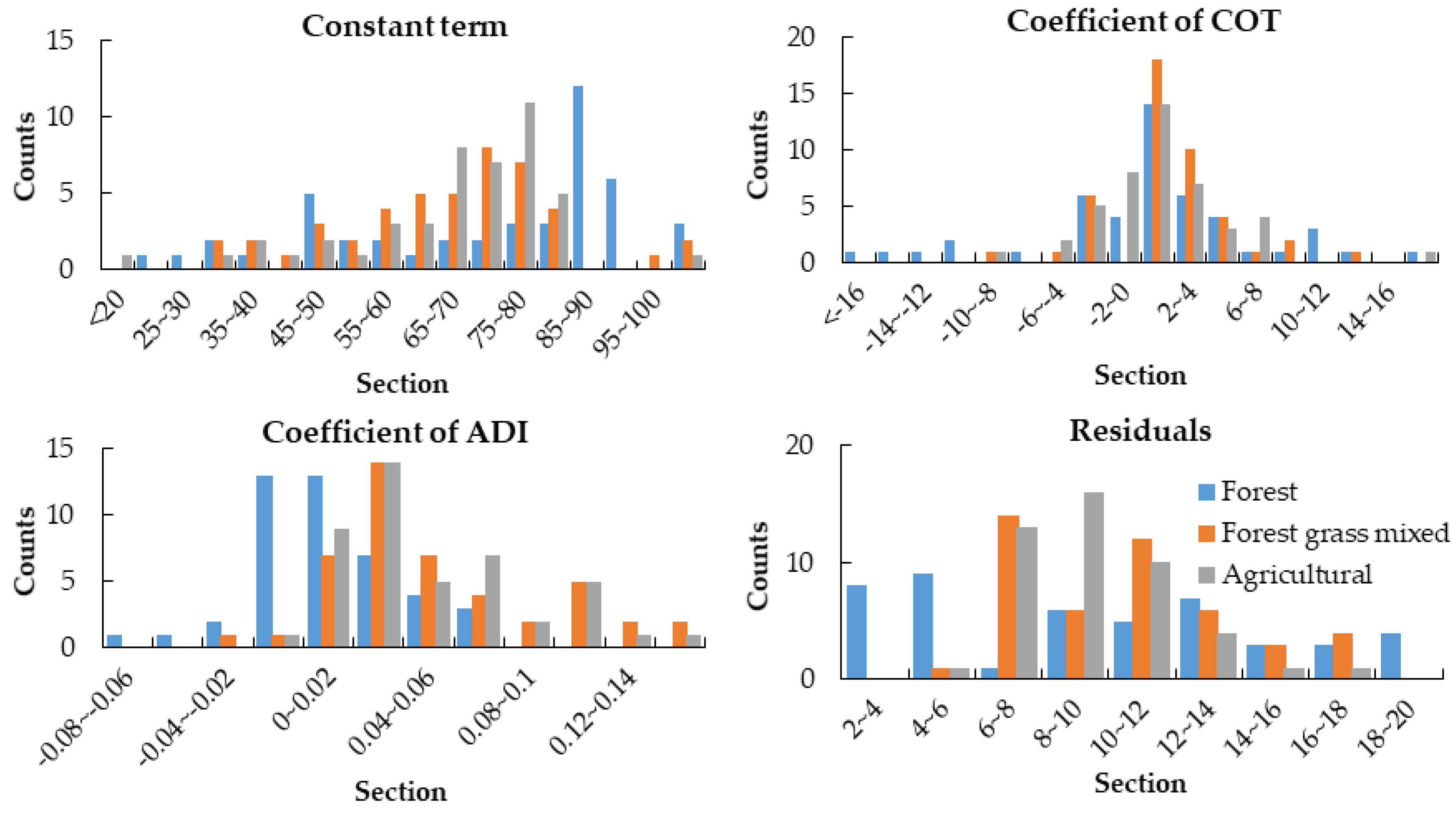
4.2. Analysis of Parameters

The parameters in Equation (4) can be obtained by the regression equation. The statistical values of parameters of forest, forest grass mixture and agricultural land in 2016 have certain regularity (

Table 2. Comparison of parameters of different land cover types in 2016.

Statistic	Land Type	Constant Term	Coefficient of COT	Coefficient of ADI	Average Residual	Absolute Residual	p Value
Average	Forest	74.55	0.32	0.02	0.00	9.61	0.00
	Forest grass mixed	68.01	0.54	0.06	0.00	10.26	0.00
	Agricultural	67.43	0.72	0.06	0.00	9.34	0.00
Median	Forest	82.68	1.04	0.01	0.00	9.83	0.00
	Forest grass mixed	69.59	1.72	0.05	0.00	10.20	0.00
	Agricultural	70.71	0.72	0.04	0.00	9.32	0.00
Variance	Forest	676.83	68.50	0.00	0.00	26.12	0.00
	Forest grass mixed	372.26	42.98	0.00	0.00	9.84	0.00
	Agricultural	272.18	23.62	0.00	0.00	5.41	0.00
Standard Deviation	Forest	26.30	8.37	0.03	0.00	5.17	0.00
	Forest grass mixed	19.52	6.63	0.04	0.00	3.17	0.00
	Agricultural	16.68	4.91	0.04	0.00	2.35	0.00

). Among the three land cover types, the average, median, variance and standard deviation of the P value and mean residual value are small. The absolute residual is around 10. It shows that 10% of them cannot be explained by the parameters in this paper. The average and median of ADI coefficients are similar, and the variance and standard deviation are very small. The ADI coefficient has little difference in different land cover types and different periods. The average and median values of COT coefficients were not significantly different, but the variance and standard deviation of COT coefficients were larger, which indicated that the coefficient of COT varied greatly among different land cover types or periods. Compared with other types of forest, the average and median values of constant and mean residual of forest are quite different. The regression parameters of forest grass mixture and agricultural are better, because the vegetation growth in agricultural land is relatively regular. The vegetation coverage rate of forest grass mixed type is relatively low, and the difference within the vegetation condition is small.

The histogram of parameters of the regression equation for each period of 2016 and different land cover type has certain regularity (Figure 6). Most of the parameters conform to normal distribution. Among them, the distribution of the constant term and absolute residual of the forest is different from other land cover types and other parameters, and they are not normal distributions. This may be due to the different sensitivity of different forest types to drought. Compared with the other two land cover types, the deviation of the regression estimation value of forest land may be relatively large.

4.3. Effectiveness Analysis of Filling

According to the filling situation of CRDI to the original VCI in 2016, the filling rate of each period was calculated (

Table 3. Filling efficiency of different land cover types.

Filling Efficiency	Total	Forest	Forest Grass Mixed	Agricultural
Over 98%	31	41	28	42
95~98%	10	2	12	3
90~95%	3	1	4	1
85~90%	1	1	1	0
80~85%	1	1	1	0

). Among them, the average filling rate of total data, forest, forest grass mixed and agricultural were 98.0%, 99.1%, 97.5% and 99.5%, respectively. The filling rate of each period is different, but the difference is not significant.

There are 31 periods with a filling rate greater than 98%, and 10 periods between 95% and 98% of total data. There are 41, 28 and 42 periods with a filling rate greater than 98%, and 2, 12 and 3 periods between 95% and 98% of forest, forest grass mixed and agriculture, respectively. The filling efficiency of these periods is quite good. The filling rate of less than 80% is poor, which was not found in 2016. The CRDI model can fill in the missing pixels of the traditional remote sensing drought index.

4.4. Rational Analysis of the Estimated Value

It is not comprehensive to evaluate the CRDI model from the perspective of filling efficiency, and whether the distribution of estimated values is reasonable should be considered. We took the CRDI in 2016 as the current CRDI, VCI in 2016 as the original VCI, and the CRDI in 2015 as the previous CRDI (Figure 7). The histogram distribution of different land cover types was analyzed and the rationality of the estimated value of CRDI is discussed through the histogram. The histogram distribution of CRDI in 2016 for different land cover type is similar to that of the original VCI and the previous CRDI.

In 2016, the total number of filled pixels accounted for 4.4% of the effective pixels, and the estimated CRDI values were mainly distributed between 40 and 80. The number of filled pixels in forest type accounted for 5.4% of the total number of forest pixels, and the estimated values in the CRDI model mainly ranged from 40 to 90. In the forest grass mixed type and agricultural type, the number of filled pixels accounted for 4.3% and 2.8% of the total number of forest grass mixed and agricultural areas respectively, and the estimated values in the CRDI model were mainly distributed between 40 and 80. The CRDI in 2016 did not change the overall distribution of the original VCI, and the range of estimated values in the CRDI model was reasonable.

4.5. Continuity Analysis of CRDI

The filling efficiency of the CRDI model is quite good, and the range distribution of the estimated value is also reasonable. In order to further explore the effect of the CRDI model, it is necessary to investigate the spatial and temporal continuity of CRDI. In the study area, the CRDI values of the pixels passed by the section line and the time series curve of the sample points were extracted. On the one hand, the trends of the curve itself were investigated, and on the other hand, the CRDI values of the current, previous and the same period previously were compared.

In the field of remote sensing, it is usually necessary to reconstruct the vegetation index curve, especially the time series curve. This is because some noises in remote sensing data will make the data fluctuation unneglectable [42]. There are many methods to reconstruct remote sensing data. We choose the WS (Whittaker smoother) method which was introduced by Eilers P.H. in 2003 [43].WS has the advantages of fast and convenient, simple parameters and it is easy to implement [44,45,46]. It has been widely used in the analysis of time series curve in the remote sensing field.

We selected the 36th period (early September) of 2016 as the sample data. The loss rate of VCI in this period is at a medium level. There is no significant difference between the original VCI and the previous VCI. Therefore, the estimated value of this period should be basically consistent with the corresponding previous and contemporaneous values. The reference value of this period of data is good.

The selected section line should pass through the missing pixels of the original VCI as much as possible and should also include some pixels that are not missing in the original VCI. Line AA’ and BB’ are located in the north and east of Guangdong respectively (Figure 8). The width of the section line is defined as five pixels, and the average value is taken as the value of the ordinate. When three or more pixels are missing, it is considered that the current pixel is missing. The sample points should be evenly distributed in Guangdong and represent different land use types. Point C is located in Leizhou Peninsula, point D is located in the west of Guangdong, and point E is located in the central part of Guangdong. The width of a single point is defined as 3 × 3 pixels, and the average value is taken as the value of ordinate. When there are five or more missing pixels, it is considered that the current pixel is missing. The first period data is taken as the starting point, and the abscissa is the number of periods of the current data.

Among all the pixels passing through line AA’, the missing pixels account for 68.1%. The trend in the current CRDI is similar to that of the previous CRDI, but the position of peak valley is slightly offset (Figure 9a). Line AA’ was divided into three parts: A1, A2 and A3. The difference between the current and previous CRDI of A1 is quite small, and the trend is similar. The CRDI value of A2 in the previous is higher than that in the current period, but the trend is still very similar, especially in the missing pixels of the original VCI data. Instead, the pixels where the data are not missing are different. The current CRDI of A3 is similar to that of the previous CRDI, but the trend of them is slightly different. In the area with more missing data in the middle section of A3, the details of the previous CRDI are more and the fluctuation is more obvious, while the current CRDI lacks some details here, and the trend is relatively stable.

Among all the pixels passed by line BB’, 59.1% were missing pixels. The trend of the current CRDI is similar to that of the previous CRDI, the peak valley position is slightly shifted (Figure 9b). However, in some areas, there is no obvious law of the two curves. Line BB’ was divided into four parts: B1, B2, B3 and B4. There was no significant difference between the current CRDI and previous CRDI of B1. The trend of the front and middle segments of B1 is similar. The previous CRDI of the tail segment has more details, and the curve has some fluctuations. As a whole, the current CRDI of B2 is higher than that of the previous CRDI. It can be seen that the floating range of the two curves is small. CRDI fluctuated more in the previous period, but it was more stable in the current period. Furthermore, the current CRDI is also less detailed than the previous CRDI. The value of current CRDI of B3 is close to that of the previous CRDI, and their trends are also very similar. The current CRDI of B4 was also close to the previous CRDI. There are some differences between the two curves in B4, but the trends of them are similar in the missing pixels of the middle and rear segment.

In general, the current CRDI and previous CRDI values of the two lines are different in different regions. However, the trend of the two lines is similar on the whole.

In 2016, point C has 3 of the 46 periods are missing, and the loss rate is 6.5% (Figure 10a). The CRDI values of point C in the current period and the same period vary from 50 to 80, both of which are small. The trend of current CRDI in the first three periods is opposite to that in the same period. However, there is little difference between the estimated value of the 2nd and 3rd period and the value of CRDI in the same period. Furthermore, the trends of the 2nd and 3rd periods of current CRDI are consistent with the 1st and 4th period. The estimated value of the 41st period is basically consistent with the data of the same period and has good continuity with the data before and after. The estimation results of the three periods are all good. The 2nd and 3rd periods of point C are continuous missing pixels, and compared with the 2nd period, the estimated value of the 3rd period has a certain deviation.

In 2016, point D has 3 of the 46 periods missing, with the loss rate of 6.5% (Figure 10b). The range of CRDI of point D in the current period is small, basically between ~70 and ~95, while the range of CRDI in the same period is large, basically between ~25 and ~80. Although the fluctuation ranges of the two curves is quite different, the trend is a little similar. There is a certain gap between the estimated values of the 2nd, 29th and 34th periods and the data of the same period, but the consistency is better with the earlier and later periods. The trend of the current CRDI before and after the 34th periods is similar to that of the same period, the estimation result of the 34th period is better. It should be noted that CRDI in 2015 showed a significant trough between the 17th and 28th periods. It can be inferred that there may be drought near point D in this period, but there is no obvious drought in 2016.

In 2016, point E has 4 of the 46 periods missing, and the loss rate is 8.7 % (Figure 10c). The value of CRDI in the current period and that in the same period fluctuated greatly, basically between 40 and 90. Compared with the same period, the estimated values of the 1st, 21st, 29th and 45th period have large gaps. However, the trend of the current period is consistent with that of the previous period in the 1st, 21st and 45th periods. These three periods have good estimation effect.

From the perspective of spatial continuity, the estimation effect of CRDI is quite good. There is a good consistency between the estimated data of the three points and the trend of the previous and later data. From the perspective of time continuity, the estimation effect of CRDI is also good.

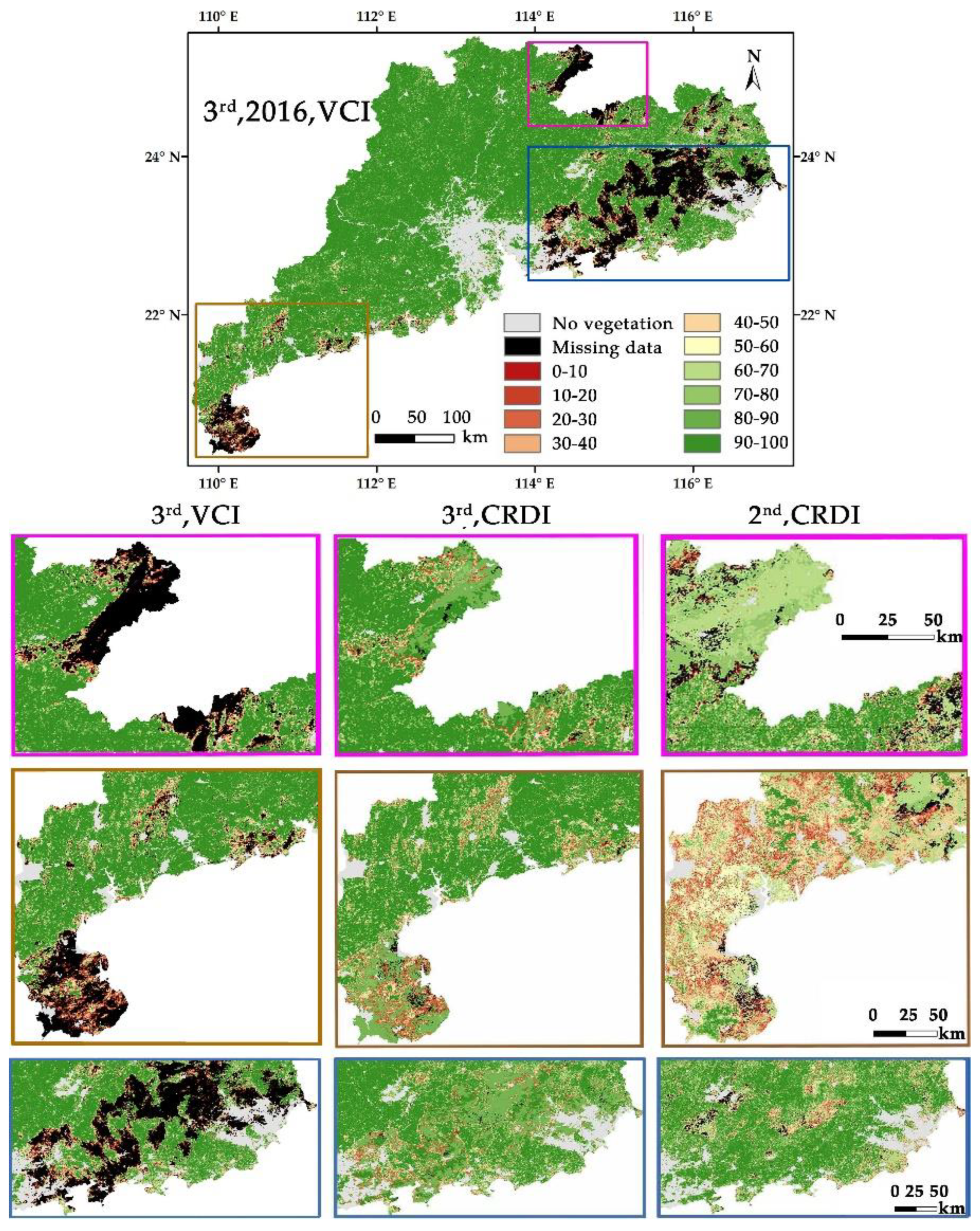
4.6. Comparison of Spatial Distribution Between CRDI and VCI

Take the 3rd (mid-January) and 15th (early April) period of 2016 as an example; in the enlarged area where VCI deficiency is concentrated, the distribution of the current CRDI, the original VCI and the previous CRDI are compared.

The value of VCI in the 3rd period of 2016 is relatively high, basically distributed above 80. The missing pixels of this period are concentrated in Leizhou Peninsula and eastern Guangdong, and the missing pixels account for 3.33% of the effective pixels. However, the loss rate of CRDI is 0.04%, most of the missing pixels can be effectively filled by CRDI model (Figure 11). The estimated values are basically distributed between 70 and 90.

In the 3rd period, the missing pixels in the pink region are mainly forest type. In the brown region, the missing pixels were mainly those of an agricultural type. In the blue region, the missing pixels were mainly those of the forest grass mixed type. The filling effects of these three regions of the estimated value are quite good. The spatial distribution of CRDI after filling are also good. There is a certain difference between the current CRDI and the corresponding previous CRDI in the second region, because the original VCI is different from the previous CRDI itself. There is a small area of CRDI in the middle of the graph with low value in the previous CRDI in the third region, but this information is lost in the current CRDI. The previous data can only be used as reference, not exactly the same as the current data.

The high value of VCI in the 15th period of 2016 was more than 80. Furthermore, there are also some low value distributions below 20, but not so much. The distribution of missing pixels is relatively scattered, accounting for 3.27% of the effective pixels. However, the loss rate of CRDI is 0.01%, most of the missing pixels can be effectively filled by CRDI model. The estimated values are basically distributed between 70 and 90.

In the 15th period, most of the missing pixels are forest or forest grass mixed type. The filling effect of these three regions of the estimated value are quite good (Figure 12). The spatial distributions of CRDI after filling are also good. There are some differences between the estimated data of the second and third regions and the corresponding previous CRDI. This is because some of the missing pixels of the current VCI are also missing in the previous period. In other words, some of the missing pixels in the 15th period were also missing in the 14th period, and these pixels were continuously missing.

5. Discussion

5.1. The Estimation of Extremum Value

Compared with the histogram of current CRDI, original VCI and the same period CRDI (Figure 7), for the CRDI of 2016, the number of estimated pixels distributed between 40 and 80 for total and different land cover types was more than the original data and the previous data. The amount of pixel distribution between 80 and 90, even between 90 and 100, is relatively small. According to the distribution trend of current VCI and CRDI in previous, more estimated pixels should be distributed between ~80 and ~100, but the number of estimated pixels in this region is less, especially in the range of 90~100. This shows that the actual estimates of many pixels that should be between 80 and 100 are smaller. In the range of 80~100, especially 90~100, the CRDI estimation results are not as accurate as other intervals.

CRDI is not so accurate for the estimation of extreme value. Usually, the same set of parameters is used to estimate the same land cover type of the same period. The data used to calculate the parameters of regression equation are distributed between 0 and 100, and the parameters are inclusive, so the parameters usually have some deviation for the estimation of extreme value.

5.2. The Influence of Continuous Loss of CRDI

For the accuracy of CRDI, the first problem of continuous missing pixels is that if the pixel cannot be estimated in the previous period, the pixel cannot be estimated in the current period (Figure 11). The second problem is that the residual of CRDI will accumulate. Due to the lack of correction of the real VCI value in the continuous missing pixels, the estimation residual will become larger and larger (Figure 11 and Figure 12).

The number of continuous missing pixels accounted for 0.47% of the total effective pixels of the 12th, 13th and 14th periods of 2016. The estimated values of continuous missing pixels and the histogram corresponding to the data before and after showed certain regularity (Figure 13a). Before and after the continuous loss of pixels, the VCI values were basically distributed between 40 and 70, and the distribution was relatively uniform. The estimated values are also distributed in this interval, but more concentrated between 50 and 60.

Among them, the distribution of the first period estimates is relatively average, which is more in line with the transition trend from the previous period to the next period (Figure 13b). The histogram of the estimated values of continuous missing pixels between 46 and 74 has certain regularity. Estimate values for the second and third periods are more concentrated than for the previous period. Compared with the first period, the second period is more concentrated between 56 and 58. Furthermore, compared with the second period, the third period is more concentrated between 56 and 60. When there are continuous missing pixels, the cumulative residual will be larger and larger, and the estimated value will be more and more concentrated on a certain value, and the difference between the missing data pixels will be smaller and smaller.

5.3. A Large Number of Data Missing Periods

If the number of missing pixels is too large, the accuracy of CRDI will be affected. The number of reference pixels used to calculate the model parameters is relatively small and concentrated. Therefore, the deviation of the calculated parameters is relatively large (more than 50%), and the estimated value also has a certain deviation. There are 11 periods with the loss rate more than 50%, accounting for about 1.6% of the total 690 periods.

68.15% of the valid pixels were missing in the 10th period of 2016, and the missing pixels were very concentrated. There is a large deviation in the estimated data of this period. However, the estimated data still have some continuity (Figure 14). In the 10th period of 2016, almost all the pixels in northern Guangdong and eastern Guangdong are missing. Due to the small number of original VCI pixels used to calculate parameters in this period, ADI plays a smaller role while COT plays a more important role in the estimation of missing pixels in this period. As a result, there are obvious edges the CRDI period below, which are the edges of the COT period. Even so, the estimated values still follow a certain distribution law, and even the left and right ends of the COT pixel edge still have a certain continuity.

5.4. Evaluation of CRDI and Future Research Directions

The main advantage of CRDI is that it can solve the problem of large blank of drought data caused by cloud cover in a traditional remote sensing model. CRDI has a good application prospect and strong applicability. In this paper, VCI, which is more advantageous in vegetation area, is selected as the remote sensing drought index. When applying the CRDI model, other drought indexes, such as CWSI, SPI or PDSI, can be selected according to the specific situation of the study area.

During the discussion of the results, we found that the CRDI model is not so accurate for the estimation of the extreme value, the continuous loss pixels and the large number of data for the missing periods. In order to improve the accuracy of the CRDI model, the following aspects can be considered for future research:

• The accuracy of basic data needs to be improved. The spatial resolution of VCI and COT is 250 m and 1 degree, respectively, COT should be resampled to 250 m. In the follow-up study, higher resolution data can be considered. The accuracy of the estimation results depends on the precision of land use/land cover data. In order to improve the accuracy, more precise land use/land cover data can be considered.
• The effect of the CRDI model in small area may be better. In calculating the parameters of the regression equation, all the pixels without missing data are used, and then the values of all missing pixels are estimated with the obtained parameters. Therefore, the intra class differences of different land cover type in the study area will affect the results of the model. The smaller the study area is, the smaller the intra class differences of different land cover type may be. Therefore, the parameters obtained are more representative of the study area. Therefore, the algorithm of the model can be improved. For example, an n × n window can be opened with the target pixel as the center, and the parameters of the model can be calculated according to the data in the window, and then the drought value of the target pixel can be estimated. However, this improvement has higher requirements for the running efficiency of the algorithm, and the running efficiency of the algorithm should also be considered. Furthermore, how to determine the size of window is also a difficult problem.

6. Conclusions

In this paper, a drought retrieval model CRDI based on COT and ADI is established for the pixels whose drought value cannot be obtained due to cloud cover during the monitoring period. The drought values of the missing pixels of different land cover types were estimated for each period. The effect of the CRDI model was evaluated from the filling efficiency of the model, the rationality of the estimated value and the temporal and spatial continuity of CRDI. Furthermore, the estimations of large missing and continuous missing periods are analyzed. The main conclusions are as follows:

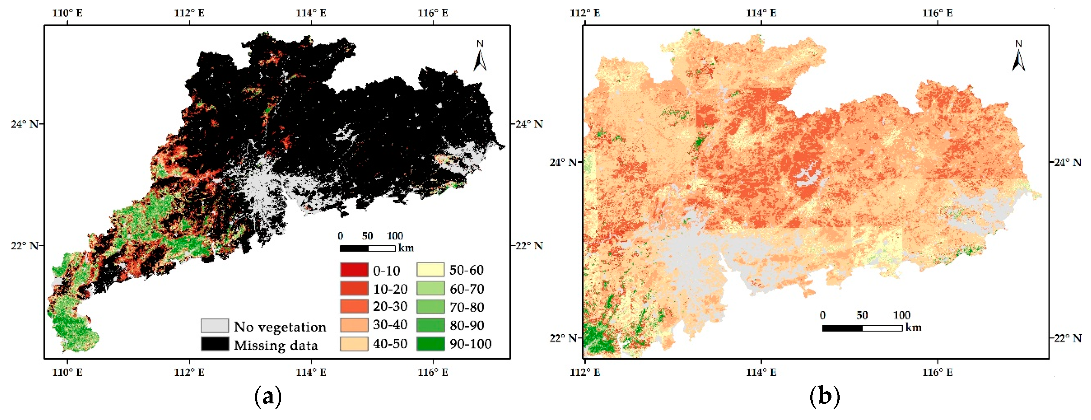
• The filling efficiency of CRDI is high. CRDI can fill most of the missing data. The average filling efficiency of total data, forest, forest grass mixed and agricultural was as high as 98.0%, 99.1%, 97.5% and 99.5%. Even for the most inefficient periods, 80% were filled.
• The estimated value of CRDI is reasonable. The range distribution of CRDI and its corresponding original VCI is similar, and the estimated value is also within a reasonable range. However, the estimated value is more concentrated than the corresponding previous and the same period data, and the estimation of extreme value is not as accurate as others.
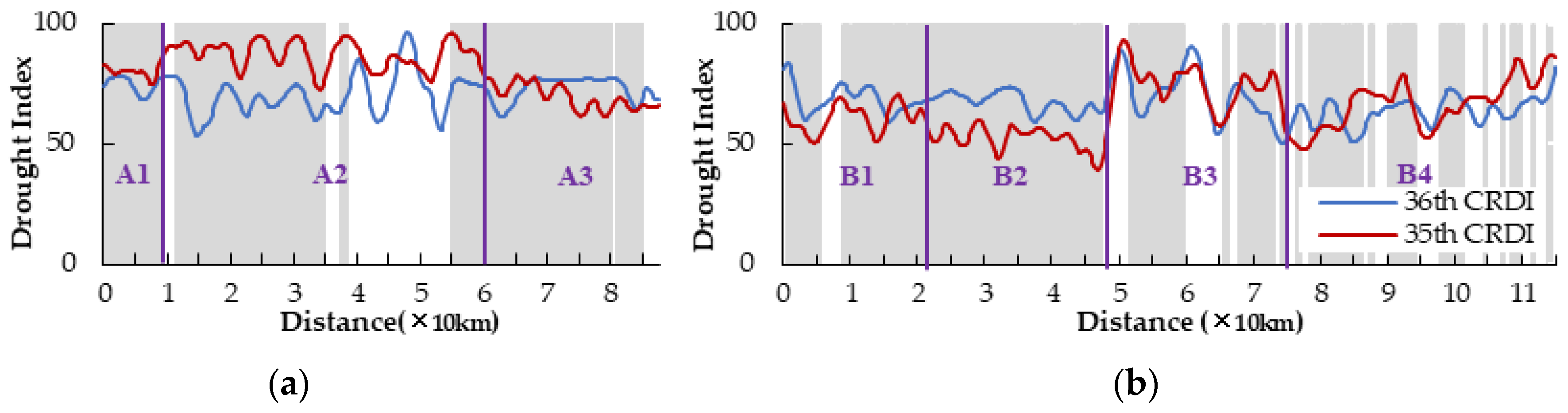
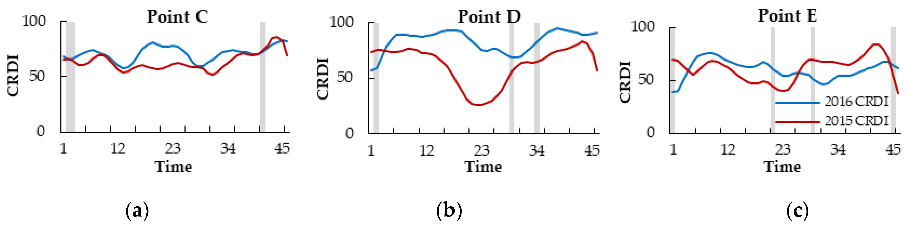
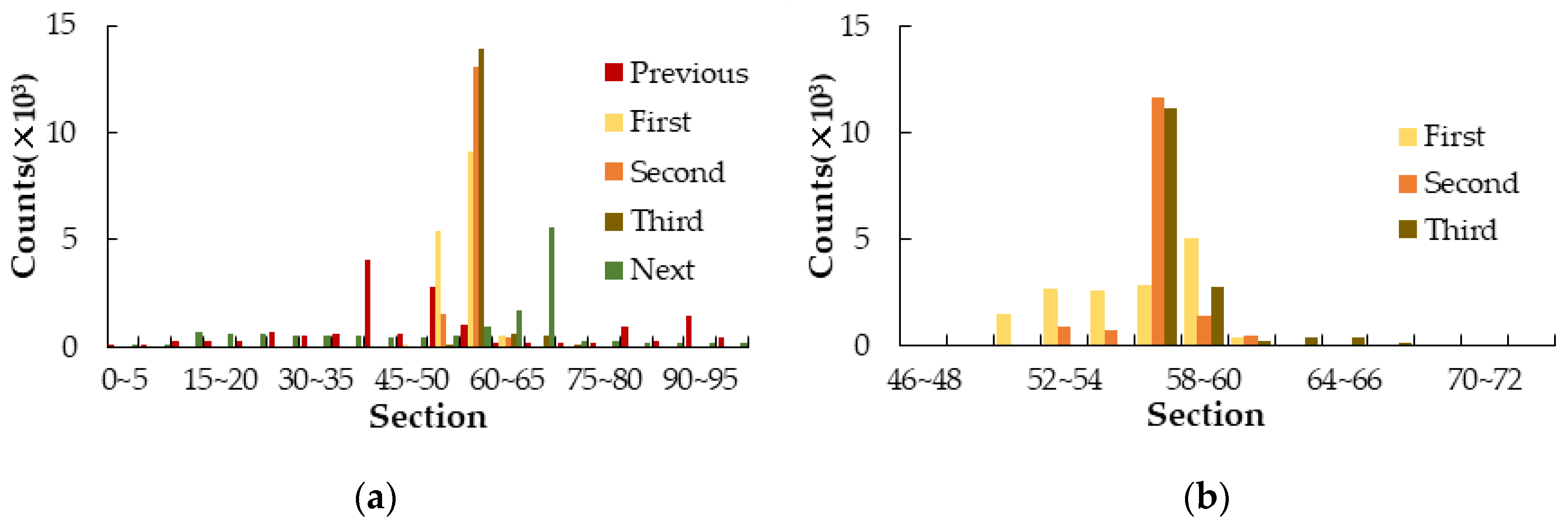
• The continuity of CRDI is quite good. The continuity of CRDI data is analyzed from the perspective of space and time by comparison section line and sample points. The trend of the section line between the current CRDI and the previous CRDI is very similar, and it is reasonable for CRDI to fill the missing areas. The trend of the CRDI curve of sample points is similar to that of the same period, and the continuity of estimated data is better than that of previous and next curve. Considering both time and space, the CRDI model has good continuity. In addition, by comparing the spatial distribution of CRDI and VCI, it is found that the estimated values have good continuity with the surrounding drought values.

References

1. Wang, J.S.; Li, Y.H.; Wang, R.Y.; Feng, J.; Zhao, Y. Preliminary Analysis on the Demand and Review of Progress in the Field of Meteorological Drought Research. J. Arid Meteorol. 2012, 30, 497–508. [Google Scholar]
2. Yuan, W.P.; Zhou, G.S. Comparison Between Standardized Precipitation Index and Z-index in China. Chin. J. Plant Ecol. 2004, 28, 523–529. [Google Scholar]
3. Bulut, B.; Tugrul, Y.M.; Cosh, M.H.; Mladenova, I. Quality control of station-based soil moisture observations in Turkey. In Proceedings of the Agu Fall Meeting, San Francisco, CA, USA, 14–18 December 2015. [Google Scholar]
4. Ford, T.; McRoberts, D.B.; Quiring, S.M.; Hall, R.E. On the Utility of In-Situ Soil Moisture Observations for Flash Drought Early Warning in the Central United States. In Proceedings of the Agu Fall Meeting, San Francisco, CA, USA, 14–18 December 2015. [Google Scholar]
5. Sehgal, V.; Sridhar, V.; Tyagi, A. Stratified drought analysis using a stochastic ensemble of simulated and in-situ soil moisture observations. J. Hydrol. 2017, 545, 226–250. [Google Scholar] [CrossRef] [Green Version]
6. Xu, Y.P.; Wang, L.; Ross, K.W.; Liu, C.; Betcrry, K. Standardized Soil Moisture Index for Drought Monitoring Based on Soil Moisture Active Passive Observations and 36 Years of North American Land Data Assimilation System Data: A Case Study in the Southeast United States. Remote Sens. 2018, 10, 301. [Google Scholar] [CrossRef] [Green Version]
7. Mihajlović, D. Monitoring the 2003–2004 meteorological drought over Pannonian part of Croatia. Int. J. Climatol. 2006, 26, 2213–2225. [Google Scholar] [CrossRef]
8. Mirabbasi, R.; Anagnostou, E.N.; Fakheri-Fard, A.; Dinpashoh, Y.; Etcslamian, S. Analysis of meteorological drought in northwest Iran using the Joint Deficit Index. J. Hydrol. 2013, 492, 35–48. [Google Scholar] [CrossRef]
9. Patel, N.R.; Chopra, P.; Dadhwal, V.K. Analyzing spatial patterns of meteorological drought using standardized precipitation index. Meteorol. Appl. 2007, 14, 329–336. [Google Scholar] [CrossRef]
10. Yang, S.; Yu, Z.G.; Su, Y. Spatial pattern of meteorological drought in China (1951–2011). J. Arid Land Resour. Environ. 2014, 28, 54–60. [Google Scholar]
11. Wang, C.L.; Chen, H.H.; Tang, L.S.; Duan, H. A Daily Meteorological Drought Indicator Based on Standardized Antecedent Precipitation Index and Its Spatial-Temperal Variation. Prog. Inquis. Mutat. Clim. 2012, 8, 157–163. [Google Scholar]
12. Cook, E.R.; Jacoby, G.C. Tree-Ring-Drought Relationships in the Hudson Valley, New York. Science 1977, 198, 399–401. [Google Scholar] [CrossRef] [PubMed]
13. Huber, K.; Dorigob, W.A.; Bauerc, T.; Eitzinger, J.; Haumann, J.; Kaiser, G.; Linke, R.; Postl, W.; Rischbeck, P.; Schneider, W.; et al. Changes in spectral reflectance of crop canopies due to drought stress. In Proceedings of the 11th SPIE International Symposium on remote Sensing, Vienna, Austria, 20–22 September 2005. [Google Scholar]
14. Rigling, A.; Bräker, O.; Schneiter, G.; Schweingruber, F. Intra-annual tree-ring parameters indicating differences in drought stress ofPinus sylvestrisforests within the Erico-Pinion in the Valais (Switzerland). Plant Ecol. 2002, 163, 105–121. [Google Scholar] [CrossRef] [Green Version]
15. Tian, Q.; Gou, X.; Zhang, Y.; Peng, J.; Wang, J.; Chen, T. Tree-Ring Based Drought Reconstruction (A.D. 1855–2001) for the Qilian Mountains, Northwestern China. Tree-Ring Res. 2007, 63, 27–36. [Google Scholar] [CrossRef]
16. Lloret, F.; Lobo, A.; Estevan, H.; Maisongrande, P.; Vayreda, J.; Terradas, J. Woody plant richness and ndvi response to drought events in catalonian (northeastern Spain) forests. Ecology 2007, 88, 2270–2279. [Google Scholar] [CrossRef]
17. Peters, A.J.; WalterShea, E.; Ji, L.; Viña, A. Drought monitoring with NDVI-based standardized vegetation index. Am. Soc. Photogramm. Remote Sens. 2002, 68, 71–75. [Google Scholar]
18. Gu, Y.; Brown, J.F.; Verdin, J.P.; Wardlow, B. A five-year analysis of MODIS NDVI and NDWI for grassland drought assessment over the central Great Plains of the United States. Geophys. Res. Lett. 2007, 34, 06407. [Google Scholar] [CrossRef] [Green Version]
19. Gu, Y.; Hunt, E.; Wardlow, B.; Basara, J.B.; Brown, J.F.; Verdin, J.P. Evaluation of MODIS NDVI and NDWI for vegetation drought monitoring using Oklahoma Mesonet soil moisture data. Geophys. Res. Lett. 2008, 35, 22401. [Google Scholar] [CrossRef] [Green Version]
20. Wang, L.; Qu, J.J. NMDI: A normalized multi-band drought index for monitoring soil and vegetation moisture with satellite remote sensing. Geophys. Res. Lett. 2007, 34, L20405. [Google Scholar] [CrossRef]
21. Wang, L.; Qu, J.J.; Hao, X. Forest fire detection using the normalized multi-band drought index (NMDI) with satellite measurements. Agric. For. Meteorol. 2008, 148, 1767–1776. [Google Scholar] [CrossRef]
22. Patel, N.R.; Parida, B.R.; Venus, V.; Saha, S.K.; Dadhwal, V.K. Analysis of agricultural drought using vegetation temperature condition index (VTCI) from Terra/MODIS satellite data. Environ. Monit. Assess. 2012, 184, 7153–7163. [Google Scholar] [CrossRef] [PubMed]
23. Sun, W.; Wang, P.-X. Further studies on vegetation temperature condition index drought-monitoring model using AVHRR data. Int. Soc. Opt. Eng. 2005, 5884, 58840F. [Google Scholar]
24. Qian, X.; Liang, L.; Shen, Q.; Sun, Q.; Zhang, L.; Liu, Z.; Zhao, S.; Qin, Z. Drought trends based on the VCI and its correlation with climate factors in the agricultural areas of China from 1982 to 2010. Environ. Monit. Assess. 2016, 188, 639. [Google Scholar] [CrossRef]
25. Kogan, F.N. Droughts of the Late 1980s in the United States as Derived from NOAA Polar-Orbiting Satellite Data. Bull. Am. Meteorol. Soc. 1995, 76, 655–668. [Google Scholar] [CrossRef] [Green Version]
26. Kogan, F. Application of vegetation index and brightness temperature for drought detection. Adv. Space Res. 1995, 15, 91–100. [Google Scholar] [CrossRef]
27. Wang, P.-X.; Li, X.-W.; Gong, J.-Y.; Song, C. Vegetation-temperature condition index and its application for drought monitoring. Editor. Board Geomat. Inf. Sci. Wuhan Univ. 2001, 26, 412–418. [Google Scholar]
28. Quiring, S.M.; Ganesh, S. Evaluating the utility of the Vegetation Condition Index (VCI) for monitoring meteorological drought in Texas. Agric. For. Meteorol. 2010, 150, 330–339. [Google Scholar] [CrossRef]
29. Liu, L.M. The Research of Remote Sensing Drought Prediction Model Based on EOS MODIS Data; Wuhan University: Wuhan, China, 2004. [Google Scholar]
30. Tan, D.B.; Liu, L.M.; Yan, J.J. Research on drought monitoring model based on MODIS data. J. Yangtze River Sci. Res. Inst. 2004, 21, 11–15. [Google Scholar]
31. Liu, J.; Zhang, W.J.; Zhu, Y.J. Case Study on Cloud Properties of Heavy Rainfall Based upon Satellite Data. J. Appl. Meteorol. Sci. 2007, 18, 158–164. [Google Scholar]
32. Kobayashi, T.; Masuda, K. Changes in Cloud Optical Thickness and Cloud Drop Size Associated with Precipitation Measured with TRMM Satellite. J. Meteorol. Soc. Jpn. 2009, 87, 593–600. [Google Scholar] [CrossRef] [Green Version]
33. Kobayashi, T.; Masuda, K. Effects of precipitation on cloud optical thickness derived from combined passive and active space-borne sensors. AIP Conf. Proc. 2009, 1100, 267–270. [Google Scholar]
34. Wang, J. Spatial and Temporal Variation of Eco-Environment of Rice Planting Areas in Guangdong Province and Its Comprehensive Evaluation; South China Agricultural University: Guangzhou, China, 2018. [Google Scholar]
35. He, Q.J.; Cao, J.; Zhang, Y.W. Establishment and Application of Vegetation Index Sequences in Guangdong Based on MODIS Data. Meteorol. Mon. 2008, 34, 37–41. [Google Scholar]
36. Fu, C.B.; Dan, L.; Feng, J.M. Temporal and Spatial Variations of Total Cloud Amount and Their Possible Relationships with Temperature and Water Vapor over China during 1960 to 2012. Chin. J. Atmos. Sci. 2019, 41, 87–98. [Google Scholar]
37. Li, W.J.; Wang, Y.P. Analysis of the Spatial-Temporal Characteristics of Drought in Guangdong based on Vegetation Condition Index from 2003 to 2017. J. South China Norm. Univ. (Nat. Sci. Ed.) 2020, 52, 85–91. [Google Scholar]
38. Rouse, J.W.; Hass, R.H.; Schell, J.A.; Deering, D.W. Monitoring Vegetation Systems in the Great Plains with ERTS. NASA Spec. Publ. 1974, 1, 309–317. [Google Scholar]
39. Kogan, F.N. Remote sensing of weather impacts on vegetation in non-homogeneous areas. Int. J. Remote Sens. 1990, 11, 1405–1419. [Google Scholar] [CrossRef]
40. Liang, L.; Sun, Q.; Luo, X.; Wang, J.; Zhang, L.; Deng, M.; Di, L.; Liu, Z. Long-term spatial and temporal variations of vegetative drought based on vegetation condition index in China. Ecosphere 2017, 8, e01919. [Google Scholar] [CrossRef]
41. Shen, Q.; Liang, L.; Luo, X.; Li, Y.; Zhang, L. Analysis of the spatial-temporal variation characteristics of vegetative drought and its relationship with meteorological factors in China from 1982 to 2010. Environ. Monit. Assess. 2017, 189, 471. [Google Scholar] [CrossRef] [PubMed]
42. Gong, Z.J.; Liu, L.M.; Chen, J. Phenophase Extraction of Spring Maize in Liaoning Province Based on MODIS NDVI Data. J. Shenyang Agric. Univ. 2018, 49, 257–265. [Google Scholar]
43. Eilers, P.H. A perfect smoother. Anal. Chem. 2003, 75, 3631. [Google Scholar] [CrossRef]
44. Li, J.; Zhu, H. The Reconstruction of MODIS/NDVI Time Series Data in Chongqing. Sci. Geogr. Sin. 2017, 37, 437–444. [Google Scholar]
45. Zhu, H.; Li, J. Three Timed-Series NDVI Reconstruction Methods: A Case Study of Chongqing. Mt. Res. 2014, 47, 2998–3008. [Google Scholar]
46. Zhang, H.; Ren, Z.Y. Comparison and Application Analysis of Several NDVI Time-Series Reconstruction Methods. Sci. Agric. Sin. 2014, 47, 2998–3008. [Google Scholar]
Figure 1. Land use/land cover map of study area (Guangdong Province) from the international geosphere biosphere programme (IGBP) product of Moderate Resolution Imaging Spectroradiometer (MODIS) in 2016.
Remotesensing 12 03641 g001
Figure 2. Scatter diagram of vegetation conditions index (VCI) and antecedent drought index (ADI) for forest, forest grass mixed and agricultural land types in 2016.
Remotesensing 12 03641 g002
Figure 3. Scatter diagram of VCI and ADI of 19th, 33rd and 43rd periods of different land use types in 2016.
Remotesensing 12 03641 g003
Figure 4. Flow chart of the calculation of a cloudy region drought index (CRDI).
Remotesensing 12 03641 g004
Figure 5. Spatial distribution (a) and statistical chart (b) of missing data.
Remotesensing 12 03641 g005
Figure 6. Histogram distribution of parameters of different land cover types in 2016.
Remotesensing 12 03641 g006
Figure 7. Comparison of histogram distribution of current CRDI, original VCI and previous CRDI.
Remotesensing 12 03641 g007
Figure 8. VCI of the 36th period of 2016 and the position of section lines and sample points. Line AA’ starts from A and ends at A’, with a total length of about 87 km. Line BB’ starts from B and ends at B’, with a total length of about 116 km. Point C, D and E are selected from land of agriculture, forest and forest grass mixed types, respectively.
Remotesensing 12 03641 g008
Figure 9. Comparison of CRDI between the 36th and 35th periods of the section line AA’ (a) and BB’ (b). The grey parts refer to the missing data of the original 36th VCI. According to the trend of the 36th and 35th periods, the CRDI can be divided into several sections separated by purple lines, which were labeled as A1, A2 and A3 and B1, B2, B3 and B4, respectively. The blue line refers to CRDI of the 36th period, and the red line refers to CRDI of the 35th period.
Remotesensing 12 03641 g009
Figure 10. Comparison of current and same period of CRDI of point C (a), point D (b) and point E (c). The grey parts refer to the missing data of the original VCI. The blue line refers to CRDI of 2016, and the red line refers to CRDI of 2015.
Remotesensing 12 03641 g010
Figure 11. Comparison of spatial distribution of original VCI, current CRDI and previous CRDI of the 3rd period of 2016.
Remotesensing 12 03641 g011
Figure 12. Comparison of spatial distribution of original VCI, current CRDI and previous CRDI of the 15th period of 2016.
Remotesensing 12 03641 g012
Figure 13. Distribution of estimated values of continuous missing pixels: (a) compare the continuous missing data with the data before and after (b) comparison between consecutive missing data.
Remotesensing 12 03641 g013
Figure 14. Spatial distribution of VCI (a) and CRDI (b) of the 10th period in 2016.
Remotesensing 12 03641 g014