1. Introduction
The normalized difference vegetation index (NDVI) is one of the commonly used indicators to detect and indicate the status and dynamics of vegetation cover. NDVI time-series data are derived from a wide range of sources, such as MODIS, AVHRR, SeaWiFS, ASTER, Landsat (TM (the Thematic Mapper), ETM + (the Enhanced Thematic Mapper Plus), OLI (the Operational Land Imager)), and sentinel-2 MSI, which have been widely investigated and applied from regional to global scale [
1,
2,
3,
4,
5,
6,
7,
8,
9]. Due to technological and budget limitations, the current NDVI datasets cannot simultaneously meet the needs of high spatial and temporal resolution [
10,
11,
12]. In recent years, although the widespread application of UAV (Unmanned Aerial Vehicle) technology and the successive launch of new satellite systems (for example, Sentinel-2) provide a valuable supplement for traditional satellites, we are still lacking NDVI time-series data with high spatiotemporal resolution [
12,
13,
14]. Therefore, spatiotemporal fusion is of great significance for the study of long-term land surface dynamic processes in a complex environment.
When using spatiotemporal fusion technology to produce NDVI data with high spatiotemporal resolution, there are two blending strategies: blend-then-index (BI) and index-then blend (IB). Research has shown that the IB strategy will become the main strategy for producing NDVI data with high spatial resolution. The IB strategy has three advantages [
15,
16,
17]: (1) The IB strategy only fuses one band, and the calculation cost is low. (2) NDVI data can eliminate most of the effects related to instrument calibration, solar angle, terrain, cloud shadow, and atmospheric conditions, and enhance the response to vegetation so that the IB strategy can better reduce noise. (3) Because the BI strategy needs to fuse the two bands required for NDVI calculation, there is more error transmission. In addition, the short-term change of NDVI data can be considered linear, and it is reasonable and feasible for the IB strategy to use NDVI data instead of reflectance [
18].
At present, there are many spatiotemporal fusion models that can obtain NDVI time-series data with high spatiotemporal resolution [
12,
19]. Where the land cover remains unchanged and there is less landscape disturbance (hereafter called “phenological change”), several models can accurately and effectively predict phenological changes. For example, the spatial and temporal adaptive reflectance fusion model (STARFM) [
10], spatiotemporal adaptive algorithm for mapping reflectance change (STAARCH) [
20], enhanced STARFM (ESTARFM) [
11], spatiotemporal integrated temperature fusion model (STITFM) [
21], and spatial and temporal reflectance unmixing model (STRUM) [
22]. However, for land cover change with shape changes (hereafter called “shape change”), such as during urbanization, deforestation, reforestation, wildfires, and floods, the above models struggle to capture and predict these changes. To overcome these difficulties, researchers have successively proposed a series of models, such as the unmixing-based spatial-temporal reflectance fusion model (U-STFM) [
23], flexible spatiotemporal data fusion (FSDAF) model [
24], sparse-representation-based spatiotemporal reflectance fusion model (SPSTFM) [
25], hierarchical spatiotemporal adaptive fusion model (HSTAFM) [
26], spatiotemporal fusion network (StfNet) [
17], prediction smooth reflectance fusion model (PSRFM) [
27], and robust adaptive spatial and temporal fusion model (RASTFM) [
28]. Although these BI models produce competitive results, the model based on IB is more suitable for NVDI fusion [
18].
Currently, some spatiotemporal fusion models have been designed to produce NDVI data with high spatiotemporal resolution based on the IB strategy, such as the LAC-GAC NDVI integration [
29], the NDVI linear mixing growth model (NDVI-LMGM) [
18], the NDVI Bayesian spatiotemporal fusion model (NDVI-BSFM) [
30], the improved flexible spatiotemporal data fusion (IFSDAF) [
31], and spatial-temporal fraction map fusion model (STFMF) [
32]. Although the above models can capture the temporal changes and maintain the spatial details of NDVI data, they still have some limitations: (1) The land cover classification maps (hereafter called “classification map”) are the auxiliary data or prior knowledge needed by most spatiotemporal fusion models. At present, there are two ways to input the classification map, one is to input the classification map directly [
31], and the other is to generate the classification map automatically according to the unsupervised classification method [
24,
33]. Because the first method will increase workload and be affected by human factors, it is an efficient method to automatically generate a classification map using unsupervised classification method. Meanwhile, the classification map input of most spatiotemporal fusion models is obtained from the high-resolution NDVI at base date, such as NDVI-BSFM and IFSDAF, and the low-resolution NDVI at the prediction date are not involved. However, the input data for the classification should include the coarse-resolution observation on the prediction date, because it is the only observation that contains information of the surface changes on the prediction date [
28]. (2) The spatiotemporal fusion methods all adopt the window strategy to realize the prediction. Due to the grid effect of the window and the residual distribution error, the final prediction result will contain block effects, such as the ESTARFM [
11]. (3) Two or more pairs of cloudless basic NDVI data are needed, such as NDVI-LMGM and STFMF. Although NDVI-LMGM can complete NDVI data fusion by reusing one pair of images, the prediction accuracy is low [
31].
The majority of remote sensing data pixels are composed of several ground objects, and the spectral characteristics of most pixels are also composed of spectral values of multiple features. By consequence, the reflectance of pixels can be expressed as a function of the spectral characteristics of the endmembers and their area percentage (abundance). Assuming that the same ground object has the same spectral characteristics and linear additivity, the pixel between low-resolution and high-resolution data can be linked together with linear mixing theory [
10,
11]. In recent years, the vegetation index has also been used to predict the time change by linear mixing theory [
18,
34]. This study proposes a high spatiotemporal resolution NDVI fusion model based on histogram clustering (NDVI_FMHC) to generate high spatiotemporal resolution NDVI by using a linear mixing theory. In summary, the main contributions of this study are the following:
- (1)
The NDVI_FMHC constructs an effective fusion framework using two kinds of classification maps which are automatically generated by histogram clustering method. Due to the classification map containing coarse-resolution information of the surface changes on the prediction date, the NDVI_FMHC forms an important contribution to improve the prediction accuracy of phenological and shape changes.
- (2)
To reduce error, the NDVI_FMHC approach uses four strategies, namely, the construction of an overdetermined linear mixed model, multiscale prediction, residual distribution, and Gaussian filtering.
- (3)
We have designed a friendly and concise software interface for the NDVI_FMHC, which will be shared with interested users. The NDVI_FMHC software can directly generate NDVI time-series data with a high spatial resolution by using one pair of cloudless basic NDVI data but with less computational costs and prior knowledge.
2. Method
Before introducing the method, a brief description of the symbols used in the model is provided to facilitate the reader’s understanding (
Table 1).
2.1. Spatiotemporal Fusion Framework
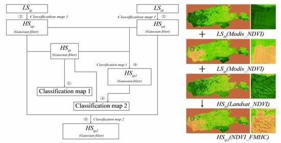
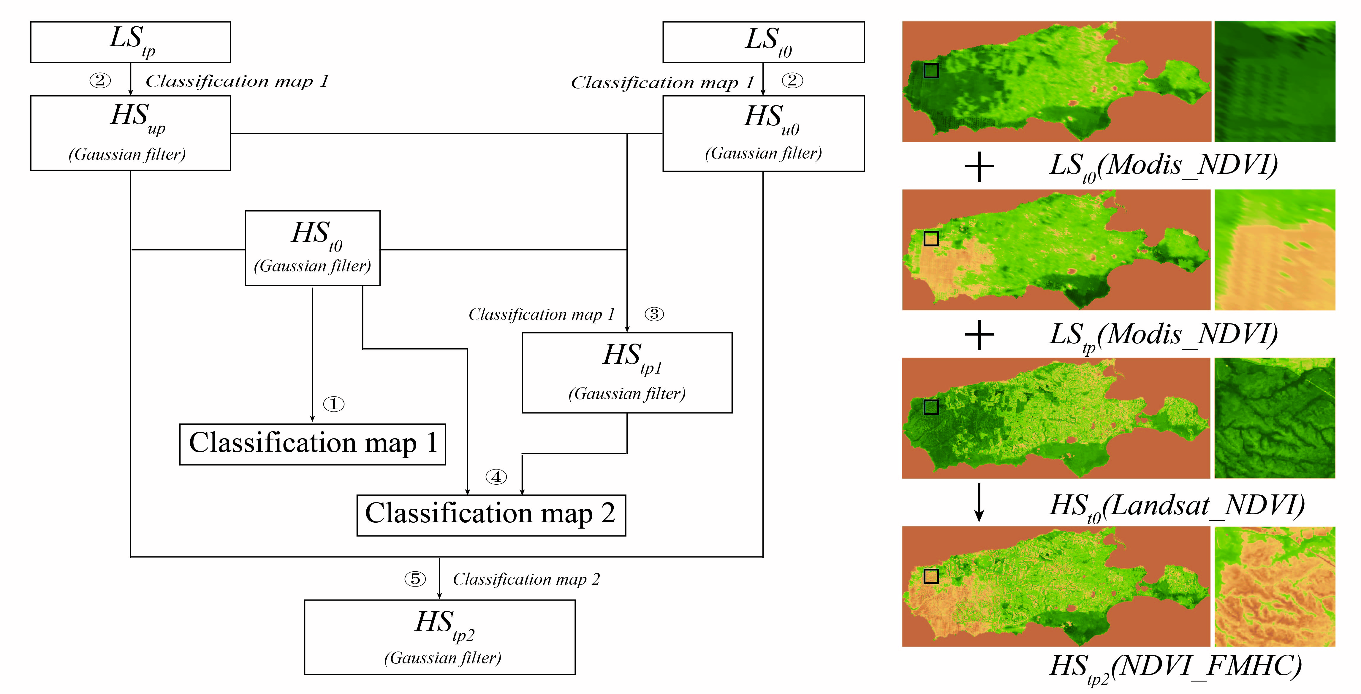
As the input data of the spatiotemporal fusion model, the quality of the classification map is crucial to the accuracy and robustness of the fusion results. Most models assume that the type of land cover cannot change during spatiotemporal fusion; however, this assumption is unreasonable in some situations, such as floods and fires. This study uses hierarchical clustering to provide land cover for NDVI data fusion through local histogram features and generates two kinds of classification maps, in which classification map 1 is used for predicting , which is directly generated from , and classification map 2 is used for predicting which is generated from and . An effective high spatiotemporal NDVI data fusion framework based on histogram feature clustering is constructed using the above two classification maps.
Based on the , and , the NDVI_FMHC approach constructs an effective fusion framework using two kinds of classification maps to predicting high-resolution NDVI data (). , and all need to be preprocessed with the same geometric correction and atmospheric correction. The spatiotemporal fusion framework consists of five steps: ① Classification map 1 is generated by hierarchical clustering according to the local histogram features based on ; ② Combined with classification map 1, and are up-sampled using a linear mixing model to obtain the and with the Landsat resolution as ; ③ Based on , and , using classification map 1, the first high spatial resolution NDVI data at () are predicted by the linear mixing model; ④ Combined with and , classification map 2 is generated by hierarchical clustering according to the local histogram features; ⑤ Based on , , using classification map 2, the second high spatial resolution NDVI data at () are predicted through the linear mixing model. In the above five steps, the , and , , and are all processed by Gaussian filtering.
2.2. Feature Description of Land Cover Classification
The NDVI_FMHC automatically generated a classification map by the hierarchical clustering method, in which a local histogram is used as the feature to classify pixels. In the first three steps of the NDVI_FMHC, due to the lack of high spatial resolution information at , a 3 × 3 moving window based on only is used to build classification map 1 produced by a 16-dimensional local histogram feature. After obtaining , classification map 2 is generated based on and , in which each moving window at the corresponding position generates a 16-dimensional local histogram, and then expands to a 32-dimensional local histogram. Therefore, classification map 2 contains both phenological information without shape change and land cover change information with the shape change at and , which helps improve the accuracy of the fusion result.
2.3. Estimation of NDVI Change with a Linear Mixture Model
Although the variation in NDVI over time is complex, it satisfies the linear change hypothesis in the short term [
18]. The NDVI increment of the coarse pixel
is defined as
According to linear mixing theory, the NDVI of the coarse pixel is a linear superposition of the fine pixel, from which the relationship between the short-term change of the coarse pixel and the fine pixel NDVI can be obtained, as follows:
In Equation (2), l is the count of classes and
is the increment of the coarse pixel NDVI from
. It should be noted that the coarse pixel here is not the original low-resolution data pixel, but a new coarse pixel composed of a certain number of fine pixels based on
and
(detailed in
Section 2.5).
is the abundance of the l category in the coarse pixels
. When obtaining
, the abundance is calculated from classification map 1, and when predicting
, the abundance is calculated from classification map 2.
is the increment of the fine pixel NDVI of category l from
. The least-squares method is used to solve Equation (2) to obtain the optimal solution of
.
2.4. Residuals and Its Allocation Formed by Predicting Time Changes
Previous studies [
24] have shown that if there is no land cover change from
, the value of NDVI fine pixels can be accurately estimated at
, while the prediction is less accurate where land cover change has occurred and large within-class variability exists. In addition, it is difficult to construct a positive definite linear mixing model due to the non-equilibrium of ground feature distribution. To eliminate the influence of multiple solutions under positive definite equations, a large window is usually used to construct the equations of the overdetermined linear mixing model. After the optimal solution is obtained by the least-squares method, although the residual error is very small, it is still not zero. The residual estimation method of the NDVI_FMHC for the prediction and true value of fine pixels NDVI is consistent with that of FSDAF [
24], and the residual distribution method is consistent with that of IFSDAF [
31,
32].
2.5. Gaussian Filtering
First, the remote sensing data inevitably contains noise due to the influence of sensor material properties and the working environment. Second, while solving the linear mixed model using the least squares method, additional noise is generated. Therefore, The NDVI_FMHC uses Gaussian filtering to remove the noise of
,
,
,
and
. The formula is as follows:
Gaussian filtering is mainly affected by two parameters when removing noise, which are Gaussian kernel size and standard deviation (σ). Gaussian kernel size is a 3 × 3 fine pixel window, and σ is determined through multiple experiments. In addition, is the value of the fine pixels at after Gaussian filtering.
2.6. Block Effect Elimination and Final Prediction
The spatiotemporal fusion methods all adopt the window strategy to realize the prediction. Due to the grid effect of the window and the residual distribution error, the final prediction result will contain block effects, similar to the ESTARFM algorithm [
11]. To eliminate the block effect, the NDVI_FMHC uses multiple different numbers of fine pixels to form new coarse pixels based on
and
, and uses the arithmetic average of several prediction results as the final prediction result (hereafter called “multiscale prediction”). Specifically, the NDVI_FMHC introduces a new parameter (coarse pixel width) to determine the size of a new coarse pixel. If the input value of the coarse pixel width is k (k ≥ 3), the size of the new coarse pixel has three values, and the resolutions are k × 30 m, (k + 2) × 30 m, and (k + 4) × 30 m (fine pixel size is 30 m). Values above the three coarse pixel width are used to make three predictions respectively, obtaining three parallel
, which can be marked as
,
, and
. For instance, when the value of k is 4 and the fine pixel size is 30 m,
is predicted using the new coarse pixel of 120 × 120 m according to the framework of the NDVI_FMHC (
Figure 1), then
and
are predicted using the new coarse pixel of 180 × 180 m and 240 × 240 m, respectively. The final prediction result of Landsat_NDVI is as follows:
is the final prediction result.
5. Discussion
The study integrates multi-source remote sensing data (MODIS_NDVI and Landsat_NDVI) to obtain NDVI time-series data with high spatiotemporal resolution and study the long-term dynamic processes of the surface environment. In general, the most common natural changes on the land surface are phenological changes, simultaneously accompanied by dramatic land cover changes. Due to water levels rising or falling, fire hazards, floods, urban expansion, and deforestation, shape changes of land cover also frequently occur. During spatiotemporal fusion, the prediction of phenological changes is relatively easy, while the prediction of these shape changes is extremely difficult. Therefore, it is of great significance to understand the accurate, automatic, and robust prediction of complex shape changes in various landscapes for comprehensive monitoring of the surface dynamics.
5.1. Prediction Advantages of the NDVI_FMHC
The changing pattern of NDVI is determined by biotic factors (e.g., vegetation type) and environmental factors (soil, temperature, and precipitation). However, environmental factors play a more significant role than biotic factors, and in a small area, NDVI change can be assumed to be similar within the same type of land cover. Therefore, NDVI-LMGM assumes that within a short period, NDVI values of adjacent pixels of the same land cover exhibit the same linear changes [
18]. If only phenological changes occurred, this assumption would be reasonable, but the prediction results will have a large error when shape changes and existing variations occur within the class. The FSDAF [
24] has designed a new weighting function reallocating residuals to areas with shape changes reducing errors. The NDVI_FMHC proposes a new spatiotemporal fusion framework to solve this problem based on classification map 1 and classification map 2, in which classification map 1 is obtained by
and classification map 2 is obtained by combining
and
. Compared with classification map 1, classification map 2 further refines the land cover types and its changing characteristics, which can distinguish shape changes that did and did not occur during the prediction period. Therefore, the abundance calculated by classification map 2 is more reasonable, and the time variation of the terminal element solved by the linear mixture model has better robustness and higher accuracy.
It is necessary to select a suitable classification method to classify and obtain an accurate classification map, which is the basis of the spatiotemporal fusion model. Currently, some spatiotemporal fusion models select similar pixels based on the threshold of spectral distance to obtain classification maps, such as STARFM and ESTARFM [
11,
24]. Because the threshold is empirical, it is difficult to accurately capture the boundaries of different land cover types owing to different objects with the same spectrum, especially NDVI. There are also some spatiotemporal fusion models using ISODATA [
18,
24] or the K-Means method [
2] to perform unsupervised classification to obtain classification maps. However, the ISODATA method needs many parameters, and the input value is not easy to determine, and K-Means is easily affected by the initial value. Hierarchical clustering is also widely used in image segmentation and classification owing to ease of use and defining similarity rules [
40,
41], and the NDVI_FMHC selects this method. There are many clustering methods for image classification, each of which has its own advantages and disadvantages. We have designed two features for applying clustering classification methods, including a 16-dimensional local histogram based on
, and a 32-dimensional local histogram expanded by two 16-dimensional local histograms based on
and
, which not only contains the information of land cover but also reflects the change at two moments.
Due to the grid effect of the window and error of residual distribution, the regional errors of shape changes and variations within the class are large, leading to the block effect of the prediction image. Therefore, it is very important to reduce the error between the true and predicted value for various spatiotemporal fusion models. The NDVI_FMHC uses four strategies to reduce error. First, the overdetermined equations of the linear mixed model are constructed with a large window and the optimal solution is obtained by the least-squares method which can reduce errors. Second, three times parallel prediction results are obtained to calculate the arithmetic average. It should be noted that the multiscale prediction is to fuse high and low frequency information to reduce the residual between the prediction and true value. Third, local variability of temporal change caused by land cover conversions or within-class differences is modelled well through the distribution of residuals. Fourth, Gaussian filter is applied to suppress the noise of . Although the filtering makes the prediction image much blurrier and thus reduces the actual spatial resolution, a smaller standard deviation of Gaussian filter has little influence on the blurriness and can reduce the singular points of the predicted result.
Low computational efficiency is a key factor restricting the widespread application of spatiotemporal fusion models [
12]. In terms of the tested fire area (4444.64 km
2), NDVI_FMHC and NDVI-LMGM only require 4.10 min and 2.58 min, while ESTARFM and FSDAF require 105.37 min and 111.52 min. Due to multiple parallel processing of NDVI_FMHC, the computational efficiency is lower than that of NDVI-LMGM. However, the calculation efficiency of NDVI_FMHC is much higher than that of ESTARFM and FSDAF for two main reasons, including the use of advanced programming strategies, such as parallel computing, and no need to use ENVI and ArcMap software, reducing the function module calling time in the prediction process.
5.2. Optimal Parameters of the NDVI_FMHC
To obtain the best prediction effects and spend the least time, a large number of trial and error experiments were performed for the first four groups of test datasets, and the optimal parameters of the NDVI_FMHC were determined involving four main parameters: count of classes, distance calculation method, coarse pixel width, and Gaussian filter parameters. The optimal parameters of the NDVI_FMHC are based on MODIS and Landsat data while might need to be adjusted by future users to other satellite data spatiotemporal fusion.
The count of classes of hierarchical clustering based on histogram features is determined by users according to experience, and it is valuable to test the influence of count of classes on prediction accuracy.
Supplemental Table S1 is the quantitative index evaluation table from 2 to 10 count of classes. In terms of trends, AAD, AE, and RMSE of cultivated land and flood areas decrease rapidly first with the increase in count of classes, and then tend to stabilise, while the changes in r and SSIM are opposite; AAD, AE, and RMSE of forests and urban areas increase slowly at first with the increase in count of classes, and then increase rapidly, while the changes in r and SSIM are opposite. In comparison, when the count of classes is four, the prediction effects of the NDVI_FMHC are relatively satisfactory.
When NDVI is classified by hierarchical clustering based on histogram features, the relationship between feature points in feature space is measured by pairwise distances. Therefore, the definition of distance measurement is of great significance to the study of the structure of feature space. In this study, we have analyzed the performance of six different distance measures including KL,
,
,
, ∩, and
[
42]. By analyzing the quantitative index evaluation tables of six different distance measures (
Table S2), for different distance measures, the difference in prediction results of the NDVI_FMHC is very small, indicating that the different distance measures have little effect on the prediction performance of the new spatiotemporal fusion framework. In addition, because
and
have the smallest AAD, AE, and RMSE, and the largest r and SSIM, it is recommended that
and
are the formulas of distance measurement for the NDVI_FMHC.
Coarse pixel width is a parameter to determine the size and change in coarse pixel width, which is also one of the important parameters of the NDVI_FMHC.
Supplemental Table S3 is the quantitative index evaluation table under the width from 3 to 10 coarse pixels. In terms of trends, AAD, AE, and RMSE of the four test areas slowly decrease with the increase in the coarse pixel width, and then increase rapidly, while the changes in r and SSIM are opposite. The coarse pixel width may introduce a large error to the prediction result, leading to the decrease in the prediction effect, and the recommended coarse pixel width is 3 or 4.
Gaussian filtering is a kind of linear smoothing filter, and the smoothing degree depends on the standard deviation. The larger the standard deviation, the more dispersed the distribution, and the filter effect will be closer to the mean filter; the smaller the standard deviation, the more concentrated the distribution, and the filter effect will be weaker.
Supplemental Table S4 is the quantitative index evaluation table under the change in standard deviation from 0.1 to 1. In terms of trends, AAD, AE, and RMSE of the four test areas first decrease with the standard deviation, then increase, and reach the minimum value at 0.5 or 0.6, while the change rule of r and SSIM is opposite, which means that the standard deviation is too small to eliminate the noise mixed with the prediction results, while the standard deviation is too large, some of the accurate values in the prediction results will also be eliminated as noise. Therefore, the recommended standard deviations are 0.5 and 0.6.
5.3. Limitations of the NDVI_FMHC
The NDVI_FMHC shows good robustness and prediction accuracy in predicting phenological changes and shape changes; however, the following aspects still need to be improved. First, in urban expansion, shape changes are generally large in number and small in size, and the low-resolution NDVI of the predicted date and a pair of high and low-resolution NDVI of the basic date did not record these changes, increasing the prediction difficult. Second, because MODIS and Landsat images were collected at an interval of approximately 0.5 h and the flood occurred very quickly, the range of shape changes recorded by two kinds of NDVI is not consistent, causing unsatisfactory fusion results. Third, for the multiple types of land cover converted into a single type due to the fire, although current fusion models can capture the overall shape change, the local prediction effect is not ideal because the prediction results still retain the texture information of the basic Landsat_NDVI. If we can propose a better new framework or add auxiliary data (other high-resolution images), the prediction accuracy of the above complex shape changes may be improved.
6. Conclusions
This study proposes an effective high spatiotemporal NDVI fusion model based on histogram feature clustering to obtain NDVI data with high spatiotemporal resolution. Compared with the three fusion models of ESTARFM, NDVI-LMGM, and FSDAF, we also have found that except for fire areas, the NDVI_FMHC has the highest prediction accuracy, the best spatial detail retention, and the strongest ability to capture shape changes. The new spatiotemporal fusion framework proposed by the NDVI_FMHC can better predict phenological changes and shape changes because classification map 2 is obtained by combining and , which can distinguish shape changes that occurred from those that did not occur during the prediction period. Meanwhile, the NDVI_FMHC also uses four strategies to reduce the error, including the construction of the overdetermined linear mixed model, Multiscale prediction, residual distribution, and Gaussian filtering.
Although the NDVI_FMHC has good robustness and prediction accuracy, it still needs to improve. For example, this model cannot predict small changes, instantaneous changes caused by floods, and the shape changes from the multiple types of land cover converted into a single type. In addition, this study does not test the fusion performance of the NDVI_FMHC on other vegetation indexes. We have designed a friendly and concise user interface for the NDVI_FMHC, which will be shared (
https://github.com/xingxuejun1989/NDVI_FMHC) for interested users.

 ,
, 


