Meteorological OSSEs for New Zenith Total Delay Observations: Impact Assessment for the Hydroterra Geosynchronous Satellite on the October 2019 Genoa Event

Abstract

Along the Mediterranean coastlines, intense and localized rainfall events are responsible for numerous casualties and several million euros of damage every year. Numerical forecasts of such events are rarely skillful, because they lack information in their initial and boundary conditions at the relevant spatio-temporal scales, namely O(km) and O(h). In this context, the tropospheric delay observations (strongly related to the vertically integrated water vapor content) of the future geosynchronous Hydroterra satellite could provide valuable information at a high spatio-temporal resolution. In this work, Observing System Simulation Experiments (OSSEs) are performed to assess the impact of assimilating this new observation in a cloud-resolving meteorological model, at different grid spacing and temporal frequencies, and with respect to other existent observations. It is found that assimilating the Hydroterra observations at 2.5 km spacing every 3 or 6 h has the largest positive impact on the forecast of the event under study. In particular, a better spatial localization and extent of the heavy rainfall area is achieved and a realistic surface wind structure, which is a crucial element in the forecast of such heavy rainfall events, is modeled.

1. Introduction

The Mediterranean region is frequently struck by severe rainfall events causing numerous casualties and several million euros of damage every year [1]. In particular, the unusually complex terrain of the western Mediterranean areas, characterized by high mountains close to the coastlines (Alps, Apennines, Massif Central, Pyrenees), can enhance or trigger the deep convective processes often originating over the warm sea in the fall season [2,3,4]. Among the heaviest rainfall phenomena of this region, there are Mesoscale Convective Systems (MCSs). On short time-scales, their relevance is due to their high probability of triggering floods and flash-floods, with significant societal impacts, often combined with numerous shortcomings in their forecast [5,6,7]. Being characterized by very high accumulated rainfall depths, they are also responsible for a large proportion of rainfall on annual time-scales. Climate projections suggest that their importance, in terms of frequency and intensity, is likely to increase in a warming climate. Recent studies demonstrate a strong sensitivity of the predicted climate impacts to the numerical representation of MCSs, with current climate models not generally capturing MCSs well enough [8]. Thus, improving the forecast accuracy of MCSs is a fundamental step towards managing their social and economic damage on both the short and the long term.

The advance of Numerical Weather Prediction (NWP) models to increasingly higher grid spacing (km and sub-km) is paving the way to potential new synergies with space-borne systems. On the one hand, to drive high resolution NWP models, high resolution input data and boundary conditions are needed. On the other hand, the present state-of-the-art high resolution NWP models coincide with the increasing availability of space-borne observational data sources characterized either by high spatial resolution (e.g., the Sentinel missions developed in the Copernicus program framework) or by a high temporal resolution (Global Navigation Satellite System, GNSS).

In this context, the Synthetic Aperture Radar (SAR) Interferometry (InSAR) technique [9,10,11,12] applied to Sentinel-1 data enables the retrieval of information on a wide range of spatial scales of the potentially highly turbulent atmospheric water vapor field [13,14,15,16,17,18]. Many studies demonstrate the positive impact of assimilating Integrated Water Vapor (IWV) (measured in kg m${}^{-2}$) or, equivalently, Zenith Total Delay (ZTD) [m] observations in the forecast of heavy rain, both from InSAR [19,20,21,22,23], and from GNSS [22,24,25,26,27]. Hence, it is expected that feeding NWP models with EO (Earth Observation) data-derived ZTD maps combining high spatial resolution and short revisit time can represent a breakthrough in the ability to forecast extreme weather events. However, nowadays, such space-borne observations with concurrently high spatial and temporal resolutions are not available yet. On the one hand, Sentinel-1 ZTD maps have a very high spatial resolution [13,16] but a too low temporal one, of the order of some days. On the other hand, GNSS ZTD timeseries are point measurements characterized by a coarser resolution (on the order of 30 km at best, much less in some regions) but they reach a temporal resolution of 30 s [22].

In the future, InSAR data at high temporal resolution (daily, or sub-daily) could be provided by geosynchronous satellites. The geosynchronous C-band SAR mission called Hydroterra is currently a phase 0 candidate mission for the 10th Earth Explorer Programme of the European Space Agency (ESA). Hydroterra aims to observe the key processes of the daily water cycle by supplying frequent images (e.g., 1–12 h repeat time) at 1–3 km resolution. The geosynchronous orbit is expected to cover Europe and Africa. One of its main scientific objectives is to improve the physical insight and, therefore, the predictive capability of heavy rainfall and its possible consequences (floods, landslides) by providing estimates of ZTD, as well as of soil moisture, flood extent, and the presence of melting snow [28].

Concerning soil moisture, the added value of Hydroterra-derived estimates has been discussed in Cenci et al. [29]. To the best of our knowledge, a similar kind of analysis has never been carried out for ZTD estimates from Hydroterra observations and their impacts on the predictive capability of severe hydro-meteorological events. In this work, to assess the added value of high resolution/high frequency ZTD estimates using future Hydroterra observations, a set of Observing System Simulation Experiments (OSSEs) is built. An OSSE is a numerical experiment conducted with a numerical prediction model (in this case a NWP model) and a data assimilation system that ingest simulated rather than real observations. Thus, a simulated scenario is used as reference instead of real-world observations, as explained in Section 3. The OSSE approach is widely used to estimate the impacts of the proposed designs of new satellites or new kinds of observations [30,31]. However, this is the first time that an OSSE is used to evaluate the potential of the Hydroterra data for NWP applications. In particular, the OSSEs are used both to understand the best way to assimilate this new kind of observation with the state-of-the-art data assimilation systems and to assess the most useful spatio-temporal resolution for NWP applications [32,33,34,35,36].

The aim of this work is twofold. Firstly, the sensitivity to different spatio-temporal resolutions of this new kind of ZTD observation is assessed to identify the best-performing setup in the simulation of a heavy rainfall event. Secondly, the added value of assimilating the Hydroterra-like ZTD field is compared to the forecasting skills of some experiments, where already existing ZTD observations are assimilated, namely mimicking the GNSS Italian network coverage. Beyond a traditional and an object-based validation of the rainfall forecasts, the OSSEs results are also investigated using some physical criteria that are relevant for operational activities. Despite the OSSEs not being performed in fully operational configurations, this assures the relevance of the assimilation of the Hydroterra product to operational activities.

The work is organized as follows. In Section 2, the use case is presented. Section 3 introduces the OSSE setup, a comparison between the reference run (to be used to produce the synthetic observations) and the experiment with no data assimilation, the observations to be assimilated, the assimilation techniques, the experiments, and the validation method. Results are presented in Section 4. Section 5 is devoted to the discussion and the interpretation of the results, while the conclusions are given in Section 6.

2. Case Study Description

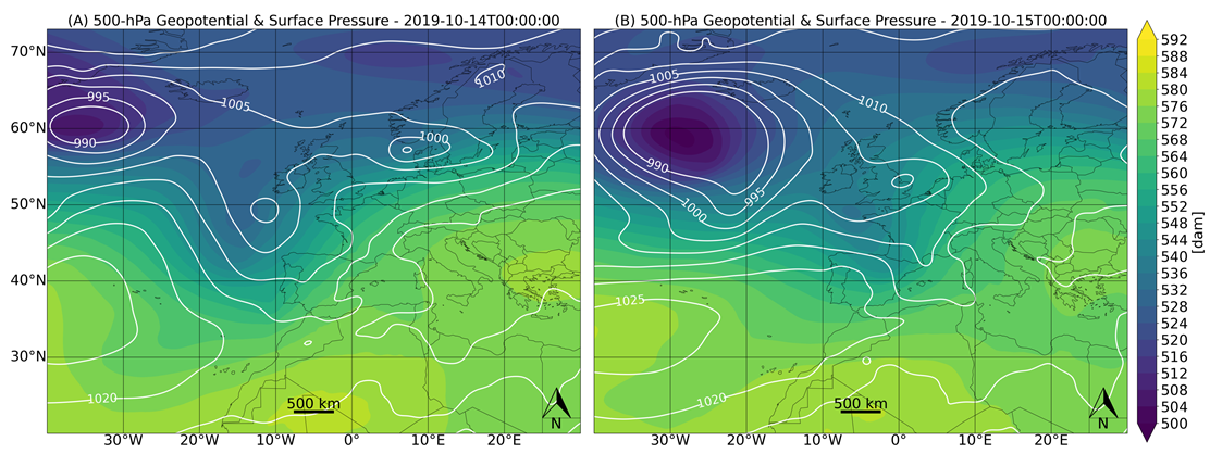
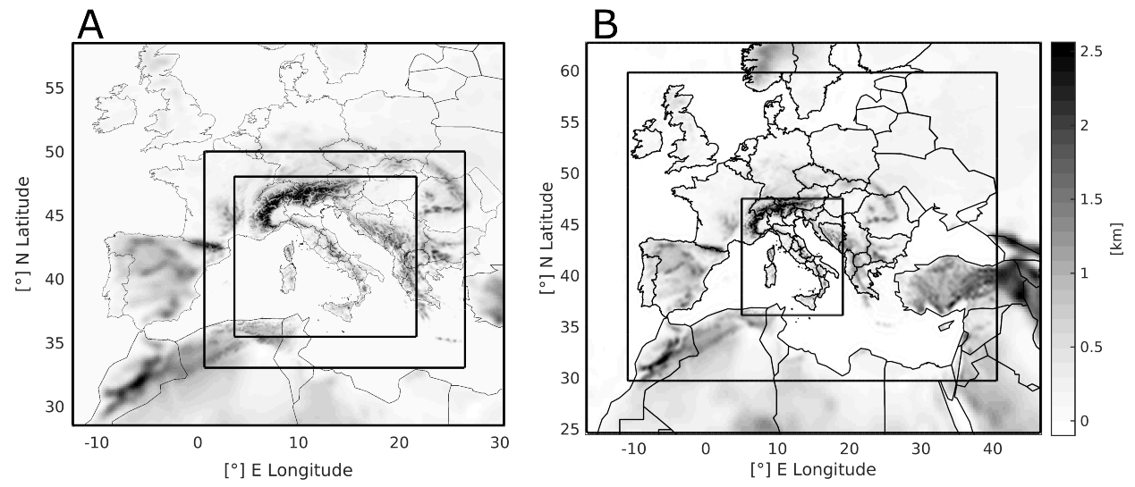
2.1. Study Area

The study area, corresponding to the territory of the Italian region called Liguria, is located along the north-western coast of Italy (see Figure 1). From a morphological point of view, the region is characterized by high mountain ranges, with a maximum height between 1000 and 2000 m a.s.l. (above sea level) that run parallel to the coast and reach their maximum height a few kilometers from the coast. The particular morphology leads to the formation of meteorological patterns specific to the region, capable of producing rainfall of relatively short duration and extremely high intensity (up to an average of 200 mm in one hour and 500–600 mm in 12 h) (see e.g., [37]). The particular meteorological situation, combined with the morphology, characterized by small basins with a high average slope, makes the region particularly exposed to flash flood risk. This type of morphology is very similar to that of several areas of the Mediterranean (e.g., Spanish, Greek, Algerian, French, and Turkish coasts) as well as the hydro-meteorological events that cause economic damage and deaths [38,39,40]. The region provides an excellent study area representative of the entire Mediterranean belt subject to flash floods.

2.2. Case Study Description

The OSSEs are performed for a high impact weather event characterized by low predictability that occurred in Italy over the Liguria region between the 14th and the 15th of October 2019. The selected case study corresponds to a back-building MCS; these are among the most important flash-flood producing storms in the Liguria region area [2,4,41] and other Mediterranean coastal regions, such as southern France [3,42] and eastern Spain [43,44]. MCSs are known to have been common in these areas also in the past [45] and there is evidence that climate change could increase their frequency [46]. It is also known that their dynamics generally develop over the sea [42,47], which can control the rainfall intensity by modifying the atmospheric stability according to the average value of sea surface temperature [48,49,50], and can influence the low-level wind field by means of the differential thermal forcing due to sea surface temperature gradients [51,52]. The low predictability of this kind of event [4,53,54] is due to the fact that small-scale meteorological processes drive their dynamical evolution. Fiori et al. [4], for example, highlight the role of the convergence line that forms over the sea when a cold and dry continental air mass coming from inland meets a warm and wet maritime air mass. The cold air mass acts as a virtual orographic barrier that lifts the unstable warm air and triggers convection.

In addition to the mesoscale lifting, the other known ingredients for the development of a back-building MCS are a relatively high level of moisture, the presence of a conditionally unstable air mass, and slowly-evolving synoptic conditions [42].

On the 14th of October 2019, a surface low pressure system located off the south-western coast of Ireland was associated with an upper-level trough extending as far south as the north African coasts, as shown in Figure 2A. At that time, a cold front was approaching the Spanish coasts and a southerly low-level flow was developing off the Ligurian coasts (not shown). Similar conditions characterized the 15th of October, see Figure 2B, where the upper level divergence of the synoptic trough was placed over the Ligurian coasts and the moist and unstable flow kept blowing from the Mediterranean Sea. Such conditions are typical of the heavy rainfall events that are known to hit northern Italy in the Autumn [55,56,57]. As outlined before, these slow-evolving synoptic conditions are necessary for the MCS development but need to be accompanied by other local forcing factors (conditional instability, low-level moisture and mesoscale lifting), which significantly challenge the predictive capabilities of current NWP modeling tools.

3. Methods and Experiments

The underlying hypothesis of this study is that by assimilating high resolution ZTD maps, the NWP model can improve its spatial representation of the low-level moisture and the conditional instability. For the event under consideration, this can affect the local dynamics, possibly helping the development of a convergence line, which can act as a lifting factor for the triggering of the back-building MCS.

3.1. OSSE Setup

The OSSEs setup is built following key points from Hoffman and Atlas [32] to guarantee its validity. The state-of-the-art Weather Research and Forecasting Model [59] (WRF, v3.8.1) is used to produce both the truth run (TR hereafter) and the forecast runs (FC hereafter), characterized by the following features:

• the TR and FC simulations are performed at different grid spacing using three two-way nested domains: 13.5, 4.5, and 1.5 km for TR (Figure 3A) and 22.5, 7.5, and 2.5 km for FC (Figure 3B). Both FC and TR have 50 vertical levels and the top of all domains reach 50 hPa;
• the TR is initialized at 00UTC of the 14th of October 2019 with the ECMWF-IFS (European Centre for Medium-Range Weather Forecasts Integrated Forecasting System) global model at 0.125° grid spacing and forced at the boundaries at an hourly frequency with the same product. The FC simulations are initialized at 00UTC of the 14th of October 2019 with the NCEP-GFS (National Centers for Environmental Prediction Global Forecast System) analysis and forecast data available at a horizontal grid spacing of 0.25° × 0.25° and forced at the boundaries every three hours;
• the microphysical parameterizations used in the two use cases are the Aerosol-aware Thompson scheme for the TR [60] and the WSM6 (WRF Single Moment six-class) scheme for the FC simulations [61];
• the Digital Elevation Model (DEM) used in the numerical simulations is smoother in the FC setup than in the TR one: the WRF default filter was applied 24 times for the TR and 36 for the FC.

The choice to use a higher resolution for the TR is mainly dictated by three considerations. Firstly, we needed to represent the phenomena under study with a sufficiently high resolution in the TR. Secondly, we wanted to have a TR ZTD field at a resolution which was as close as possible to the maximum resolution planned for the Hydroterra observations (on the order of 1 km) [62]. Thirdly, we aimed to evaluate the impact of the assimilation in a model with a setup currently used for operational forecasting activities. The remaining parameterizations (listed below) are the same for the TR and the FC experiments and follow the setup adopted in recent research [22,63,64]. They are also used in the setup implemented for an operational forecast at CIMA Research Foundation (www.cimafoundation.org/foundations/research-development/wrf.html) and include the Yonsei University scheme [65] for the planetary boundary layer turbulence closure; the RRTMG shortwave and longwave schemes [66,67,68] for radiation; the Rapid Update Cycle (RUC) scheme for the land surface model [69,70]. No cumulus scheme is activated in the two innermost domains (of both TR and FC runs), because the grid spacing is fine enough to explicitly resolve convection. An appropriate convective scheme, consistent with the boundary condition product, is activated in the outermost domain of both configurations: the Tiedke scheme [71,72] in the TR, and the new simplified Arakawa–Schubert scheme [73] in the FC experiments.

3.2. Comparison between TR and FC Open Loop

To assess the impact of ZTD assimilation at different spatial and temporal resolutions, it is necessary that the TR differs significantly from the FC_OL (the FC Open Loop simulation, i.e., with no data assimilation) and, conversely, that it represents the rainfall field well enough.

In the TR, a back-building MCS is simulated, producing accumulated rainfall depths higher than 300 mm in 12 h (Figure 4B). The simulation is very close to the back-building MCS accumulated rainfall observed by the merged radar and rain-gauges product (Figure 4A). As introduced in the previous subsection, MCSs are generally triggered by a strong and persistent (in time) convergence line over the sea, which fixes the generation of convective cells at the same position for a few hours, so that very high values of accumulated rainfall are produced [4,63,74]. Such a convergence line is visible during the main phase of the event (00, 01, 02 UTC) in the TR, as shown in Figure 5A–C.

Conversely, the FC_OL is not able to capture the correct dynamics of this event: Figure 5D–F shows that the convergence line is completely absent in the FC_OL simulation between 00 and 02 UTC. Consequently, the peak accumulated rainfall in 12 h is less than 100 mm and the precipitation is more spatially distributed (Figure 4C). The dynamics of the TR and the FC_OL seem to significantly diverge in the afternoon of the 14th of October. In fact, in the morning of the 14th both configurations model a convergence line over the sea. Later during the day, in the FC_OL, this line moves towards France and gets weaker, while in the TR, the convergence line intensifies (not shown). This is likely due to either a wrong description of the thermodynamical state of the continental air mass in the FC_OL, which prevents it from overcoming the orographic barrier and flow over the sea, or a too strong south-easterly flow from the sea, or a combination of both.

A correct representation of the convergence line in the NWP model has both dynamical and thermodynamical consequences. In fact, other than possibly producing vertical motion, the surface convergence line is also characterized by an anomalous water vapor content. This happens because the relatively dry continental air mass acts as a barrier for the moister maritime air mass [4], resulting in an accumulation of water vapor, which affects the air column stability. This is visible in Figure 5, where the 252 mm isoline of ZTD is shown in magenta. In fact, it is possible to see that, corresponding to the convergence line over the sea, a well-defined finger-like structure of high water vapor content is modeled perpendicular to the Ligurian coast in the TR (Panels A, B, C). This area of relatively high humidity, in the first place, acts as source of water for the intense heavy rain, which is one of the necessary ingredients for the development of such phenomena [42]. Secondly, the higher humidity content in the TR, decreases the atmospheric stability. In fact, over the Ligurian Sea, the maximum Convective Available Potential Energy (mCAPE) is significantly higher in the TR, O(2000 J kg${}^{-1}$), than in the FC_OL, O(1500 J kg${}^{-1}$), as discussed in Section 5. Since in the FC_OL the convergence line is not produced, also the area of higher humidity is completely absent, with the consequences for the accumulated rainfall field discussed above (Panels D, E, F).

3.3. Synthetic Observations Description and Retrieval from The TR

All the observations used in this work, namely the Hydroterra-like and the GNSS ZTD, are synthetic observations retrieved from the TR fields. ZTD can be modeled as the difference between the distance in the zenith direction covered by an electromagnetic signal assuming to be in vacuum, i.e., moving with constant velocity c, and the actual distance, i.e., that covered at the actual velocity $v\le c$. In particular, it can be expressed as the vertical integral of the atmospheric refractivity N [75], namely

$$\mathrm{ZTD}={10}^{-6}\int N\left(z\right)dz,$$

(1)

where N is a function of the pressure of dry air $p_d$, the partial pressure of water vapour e, and the temperature T along the zenith profile:

$$N\left(z\right)=k_1\frac{p_d\left(z\right)}{T\left(z\right)}+k_2\frac{e\left(z\right)}{T\left(z\right)}+k_3\frac{e\left(z\right)}{T{\left(z\right)}^2}.$$

(2)

The $k_i,i=1,2,3$ constants are experimentally determined and, in this work, their values are taken from Smith and Weintraub [76] and Bevis et al. [77], in agreement with the WRF implementation. ZTD is related to IWV through

$$\mathrm{ZTD}=\mathrm{ZHD}+\mathrm{ZWD}=\mathrm{ZHD}+\mathrm{IWV}/\Pi ,$$

(3)

where ZHD is the Zenith Hydrostatic Delay, which is substantially controlled by the surface pressure [78], ZWD is the Zenith Wet Delay, which is controlled by the highly variable water vapor content, and $\Pi$ is a conversion factor. It depends on the vertical mean value of the inverse of the temperature weighted by the water vapor density and is approximately equal to 0.15 [75,77]. To go from ZTD to IWV, thus, it is clear that additional information on surface pressure and temperature is needed. As these observations are sometimes hard to retrieve and they add processing steps that can be avoided by directly assimilating ZTD in the model, in all the experiments of this work, the assimilated variable is ZTD.

The Hydroterra-like ZTD is assimilated only over land, since Hydroterra will not retrieve ZTD over the sea. This is mainly because the ZTD InSAR maps (as the Hydroterra ones) are derived by taking phase differences for of each pixel using multi-temporal observations. The phase is the optical path delay and the own target’s signature, which should be stable in the time between the two SAR observations, in order to provide a reliable measure of the differential path delay. This does not occur when observing water, where the kinematic instability of the surface changes its radar reflectivity within milliseconds [79,80]. In SAR interferometry, water surfaces have random phase, even when observed by a very short revisit.

To obtain the GNSS-like ZTD, the TR ZTD field is interpolated on the positions of the receivers of the Italian GNSS network, with a nearest-neighbor approach. The distance between the GNSS receivers of the Italian network is between 30 and 50 km, and for a map of the receivers the reader is referred to Figure 4 of Lagasio et al. [22].

As with many heavy rainfall events, this case study was completely missed by Sentinel-1: the first observation was at 5.35 UTC of the 14th of October, too early to give some information for such very localized event, and the second one was at 5.25 UTC of the 15th of October, when the event was already over. The difficulty in finding a case study in which to assimilate Sentinel-1 ZTD map with a timely passage [22,64] is due to its very low temporal resolution with respect to the dynamics of this kind of explosive high impact weather events.

3.4. Data Assimilation Setup and Experiments Configuration

The data assimilation procedure is performed with the state-of-the-art 3DVAR WRFDA package, V3.9.1 [81]. The 3DVAR finds the optimal estimate of the atmospheric state, called ‘analysis’, by minimising an appropriate cost function that weights the background atmospheric state(coming from a NWP model run) and the observations, by their uncertainties. A technical description of the assimilation procedures used in this study is given in Appendix A.

It has been shown that when high resolution radar observations are assimilated, if the cost function is not properly constrained, such a large number of inputs can dominate the analysis result by adding large unbalanced wind increments, especially when convective systems are present [82,83]. Furthermore, the high resolution ZTD Hydroterra-like observations can lead to unrealistic dynamics, by changing the atmospheric stability and producing very vigorous vertical motion throughout the domain (not shown). This is why an additional constraint in the assimilation procedure is needed.

The additional constraint used is sensitive to the large-scale features. It is well known that one of the challenges in convective-scale data assimilation is to extract as much information as possible from the observations while maintaining the background large-scale balance. In other words, the problem is to find a way to add high resolution observational data to the initial conditions through a data assimilation system without damaging the large-scale pattern or causing spurious convection [82]. A possible solution to improve the data assimilation procedure is to use a method to minimize the imbalance problem in the 3DVAR system by adding a constraint in the cost function using information at larger scales. This is defined in terms of the departure of a high resolution 3DVAR analysis from a coarser-resolution large-scale analysis, as explained more in detail in Appendix A [82]. In this work, the version of large-scale constraint (LSC) used in Tang et al. [83] is adopted. Firstly, the GFS forecast fields (instead of analysis fields) are interpolated into the same regular grids as the outer domain via the WRF pre-processing system. Secondly, they are assimilated as bogus observations in the inner domain during the regular DA cycles. Note that, as discussed in Appendix A, not all the grid points of the large domain are considered. In particular, in the present work, the LSC sampling step is set to 45 km, corresponding to retaining every second point of the d01 grid.

The assimilation experiments are performed sampling the observation at different spatial (2.5 km, 5 km, GNSS network location) and temporal (3 h, 6 h) resolutions in all the possible combinations.

Table 1. Short description of the Observing System Simulation Experiment (OSSE)s to determine the optimal spatio-temporal resolution of the Hydroterra-like Zenith Total Delay (ZTD) observations.

Experiment	Assimilated ZTD	Obs. Resolution	DA Cycling Interval	LSC Activated
FC_OL	run without data assimilation
FC_DA_2.5 km_3 h	Hydroterra-like	2.5 km	3-h	yes
FC_DA_5 km_3 h	Hydroterra-like	5 km	3-h	yes
FC_DA_gnss_3 h	GNSS	GNSS Italian network	3-h	no
FC_DA_2.5 km_6 h	Hydroterra-like	2.5 km	6-h	yes
FC_DA_5 km_6 h	Hydroterra-like	5 km	6-h	yes
FC_DA_gnss_6 h	GNSS	GNSS Italian network	6-h	no

introduces the experiments and Figure 6 shows a schematic of the OSSEs data assimilation timing. Note that in the first 6 hours, the OSSEs have no assimilation that is due to the TR spin-up. The lower spatial resolution is set to 2.5 km (the FC resolution) because higher resolution violates the assumption of spatially independent observation errors for the $\mathbf{R}$ matrix [19,21,22].

3.5. Validation Method

The evaluation of the assimilation performances is done using the MODE tool [84,85], by comparing the TR accumulated rainfall field with the forecast fields of the other runs. The main advantage of such a validation is that the forecast is not only evaluated point-wise but also at feature level, thus overcoming the so-called “double-penalty” issue [86]. MODE identifies precipitation structures above given thresholds in both the forecast and the observed fields and performs a spatial evaluation of the model capability of reproducing the identified objects [22]. Especially for high resolution observations and cloud-resolving meteorological forecasts during deep convective events, it is preferable to use feature-based verification techniques, such as MODE, because traditional methods cannot provide a measure of spatial and temporal match between observed and forecast fields.

In this work, to evaluate the ZTD assimilation performances, 10 different indices are considered above 48 mm threshold. They include both pairs of object attributes and classical statistical scores, namely, for the geometrical indices we consider: centroid distance (CENTROID_DIST), angle difference (ANGLE_DIFF), area ratio (AREA_RATIO), symmetric difference (SYMMETRIC_DIFF), intersection area (INTERSECTION_AREA), and union area (UNION_AREA), while for the classical statistical indices we consider: Frequency BIAS (FBIAS), Probability of Detection Yes (PODY), False Alarm Ratio (FAR), and Critical Success Index (CSI). For a complete description of the indices refer to References [22,63,74].

4. Results

Looking at the 10 m wind field in the first hours of the event (Figure 7), it is possible to see that the presence or the absence of the convergence line over the sea is one of the most evident differences between the forecasts. As previously discussed, the convergence line is strong and persistent in the TR (Figure 7 Panels A, I, Q). It is interesting to underline that from a strictly forecasting view point, Poletti et al. [87] identify the presence of a convergence line over the sea as one of the most important factors that leads to the issue of a hydro-meteorological alert, as argued in what follows.

As discussed in Section 3.2, the convergence line is completely absent in the FC_OL simulation (Figure 7 Panels B, J, R). It is found that, the higher the spatio-temporal resolution of the assimilated ZTD field, the better the impact on the convergence line dynamics. In fact, assimilating the Hydroterra-like ZTD at 2.5 km grid spacing, in simulations FC_DA_2.5 km_3 h (Panels C, K, S) and FC_DA_2.5 km_6 h (Panels F, N, V), produces the most realistic convergence line. In particular, the convergence line is better defined by assimilating every 3 h, although in both cases, it is still different from the TR one. Assimilating the Hydroterra-like ZTD at 5 km grid spacing, as in the FC_DA_5 km_3 h (Panels D, L, T) and FC_DA_5 km_6 h (Panels F, N, V) runs, introduces smaller improvements in the modeling of the convergence line with respect to the previous experiments, while assimilating the ZTD at the GNSS locations in simulations FC_DA_gnss_3 h (Panels E, M, U) and FC_DA_gnss_6 h (Panels H, P, X) seems not to influence the surface wind dynamics at all. A better representation of the surface wind field in FC_DA_2.5 km_3 h (Panels C, K, S) and FC_DA_2.5 km_6 h (Panels F, N, V) is also accompanied by an increase of water vapor along the convergence line, more similar to the TR, as highlighted by the 252 mm isoline in Figure 7.

Lagasio et al. [22] showed that, for a similar back-building MCS that caused the severe Livorno 2017 flood, the ZTD assimilation from GNSS provided significant improvements in the heavy rainfall forecast. In particular, it was found that the GNSS ZTD assimilation was more effective when the wind field was simultaneously assimilated. This, together with the present findings, suggests that the coarse spatial resolution of the GNSS receivers helps in the correct modeling of the total amount of water vapor, which acts as a source for the heavy rainfall, but struggles in reproducing the fine-scale water vapor spatial distribution, that modifies the surface dynamics. This is especially true when, as in this case, the FC_OL dynamic is very far from the TR one. Thus, only by assimilating the Hydroterra-like ZTD observations at high spatial resolution, does the FC dynamic move towards the TR one, showing a convincing intense convergence line.

Thus, the effects of the ZTD assimilation on the surface wind dynamics have direct impacts on the forecast of the rainfall pattern (Figure 8). In particular, the presence of the well-defined surface convergence line when assimilating the ZTD at 2.5 km grid spacing, in experiments FC_DA_2.5 km_3 h and FC_DA_2.5 km_6 h, results in a more localized rainfall pattern (Panels B and F, respectively). Although being weaker, this is very consistent with the TR rainfall field, which shows the typical V-shape pattern of the Ligurian MCSs [4]. Assimilating a coarser ZTD product, namely the Hydroterra-like ZTD at 5 km, in the FC_DA_5 km_3 h (Panel C) and FC_DA_5 km_6 h (Panel G) runs, results in a rainfall pattern that is more localized than the OL one, but less than in the above mentioned 2.5 km experiments. With respect to the FC_DA_2.5 km experiments, the rainfall peak appears to be shifted westward. Concerning the simulation of the surface convergence field, the assimilation of ZTD at the GNSS locations, in the experiments FC_DA_gnss_3 h (Panel D) and FC_DA_gnss_6 h (Panel H), instead, maintains a more widespread rainfall pattern very similar to the FC_OL one. Note that the time intervals of the rainfall accumulation are different. In the TR, the 12 h accumulation interval is between 21 UTC of the 14th and 09 UTC of 15th of October. In the FC experiments, instead, it is between 00 and 12 UTC of the 15th of October. The reason for this is because in the FC runs, despite the assimilation procedure, a temporal shift of roughly three hours of the intense rainfall remained.

None of the FC simulations is able to reach the TR accumulated rainfall peak values. However, the assimilation of Hydroterra-like observations at 2.5 km (FC_DA_2.5 km_3 h and FC_DA_2.5 km_6 h) allows a big improvement with respect to the OL run as quantitatively highlighted by the Method for Object-Based Evaluation (MODE) rainfall validation.

Figure 9 shows statistical indices that evaluate all the objects in the whole domain of Figure 8. It is possible to see that the 48 mm threshold (Figure 9) reveals that when assimilating the Hydroterra-like ZTD observation at 2.5 km, the accumulated rainfall structure is better captured by the model (higher POD, CSI and better FBIAS and FAR), with respect to assimilating the same observation at 5 km grid spacing. In particular, assimilating at 2.5 km every 6 hours provides the lowest FAR, due to a correct spatial distribution of the rainfall field. In fact, with respect to the simulation assimilating at 2.5 km every 3 h, no rainfall overestimation is produced inland (north of 45°N, as visible in Panels B and F of Figure 8). This is probably due to the eastward displacement of the convergence line at 1UTC (Figure 7K), that is strongly reduced in the FC_DA_2.5 km_6 h (Figure 8F) forecast. In fact, the FC_DA_2.5 km_6 h has a weaker convergence line (Figure 7C,K,S) with respect to the FC_DA_2.5 km_3 h (Figure 7F,N,V), that is, however, more persistent in terms of location.

The validation in terms of the MODE geometrical indices is restricted to the core rainfall object, and not to the entire WRF innermost domain, d03. This procedure cannot be completely automated because it is specific for each event. It is also necessary to focus the validation on the area of interest, instead of the full WRF grid, in order to avoid mixing the multiple rainfall objects that appear in the simulation results, which could affect the validation results. Looking at these geometrical indices (Figure 10) it is possible to see that the angle difference (ANGLE_DIFF) of the FC_OL and the FC_DA_gnss runs are the worst ones, remarking a more widespread rainfall pattern with respect to the TR one. The CENTROID_DIST and the SYMMETRIC_DIFF highlight how the simulations assimilating Hydroterra-like observations at 2.5 km resolution (FC_DA_2.5 km_3 h and FC_DA_2.5 km_6 h) produce a better localized intense rainfall object, with a shape closer to the TR one. Furthermore, the INTERSECTION_AREA shows that the FC_DA_2.5 km_6 h has a better pattern extent.

Summarizing, it is possible to say that assimilating the ZTD Hydroterra-like observations produces the best improvement in a very challenging forecast, where the dynamical and thermodynamical differences between FC_OL and TR are large. In particular, the higher spatial resolution (2.5 km) seems to be the most effective in changing the wind dynamics and, consequently, the rainfall pattern. Both temporal resolutions of the assimilation (3 and 6 h) produce this improvement. However, the simulation assimilating every 3 h (FC_DA_2.5 km_3 h) still maintains a high FAR, due to the shifting of the simulated convergence line. Instead, a more persistent convergence line in the simulation with data assimilation performed every 6 h (FC_DA_2.5 km_6 h) gives a lower FAR (Figure 9).

5. Discussion

Only the high resolution Hydroterra-like observation experiments are capable of changing the OL dynamics enough to provide some of the main ingredients that are important to forecast this kind of back-building MCS. As previously outlined, the MODE analysis indicates that the 6-hour assimilation experiment has better performance than the 3-hour one. This suggests that a 3-hourly DA cycle may not leave enough time for a proper dynamical adjustment to the new humidity information, which can be reached with a 6-hourly cycle. Thus, it appears that the assimilation of the Hydroterra-like ZTD modifies the dynamics at the mesoscale, so that the environment is properly set for the development of the convective V-shape storm.

Due to the characteristic low predictability of this kind of event, Liguria region’s meteorological forecaster developed a check-list tool [87] to consider various ingredients indicating the possible occurrence of severe, organized, and stationary storms, like the back-building MCSs, during the operational forecasting activities.

To assess the impact of assimilating Hydroterra-like observations, the TR, OL and FC_DA_2.5 km_6 h runs are compared following Table 2 of the checklist by Poletti et al. [87]. In the first part (a) of this table, an analysis of some thermodynamic parameters such as the K-Index (KI), the Total totals (TT), the CAPE, and the Precipitable Water (PW) allows to evaluate the probability of severe thunderstorms (see Poletti et al. [87] for their definitions). If some of these parameters exceed the identified thresholds, the second part of the table (b) is used to evaluate whether the event under consideration is likely to be organized and persistent. Some of the parameters that are considered in this second part are the presence of a wind convergence line over the sea for more than 3 h, and the strength of the 950 hPa temperature (and humidity) gradient between the Po Valley and the Ligurian Sea. In this work, the use of both parts of Table 2 of Poletti et al. [87] (the checklist) allows to evaluate the impacts that assimilating the high resolution Hydroterra-like ZTD maps has on some physical quantities that are relevant for operational applications.

It is worth noticing that even if specific thresholds are identified in the Poletti et al. [87] checklist, their values need to be interpreted. For example, the CAPE parameter threshold should be modulated on the annual cycle, as summer events are usually characterized by higher CAPE values than autumn ones. Furthermore, the K-index is mentioned as a good indicator of severe and organized thunderstorms, but not for persisting ones, such as this kind of back-building MCSs. Furthermore, the TT index and the CAPE do not show a relevant predictive ability for persistent events because, for almost the whole data sets, their values fall within the respective low ranges. Thus, these indices are here used to evaluate if the simulations produce scenarios leading to severe events with respect to some metrics that are currently used for operational activities. The presence of the persistent convergence line and the surface humidity gradients are evaluated to analyse if the event can be both organized and stationary (meaning that it is more prone to generate flash floods).

A representative point within the moist and conditionally unstable air mass in the Ligurian sea is chosen to produce the Skew-T diagram and to calculate the relevant indices of the Poletti et al. [87] checklist. The virtual vertical soundings are shown in Panels A–C of Figure 11, while the corresponding surface water vapor mixing ratio maps are shown in Panels D–F. The soundings are taken in the early phase of the event, which are a few hours apart depending on the configuration, as discussed above. In particular, the virtual sounding is taken at 4 UTC in the TR experiment and at 7 UTC of the 15th of October in the FC_OL and FC_DA_2.5 km_6 h experiments.

While the TR and the FC_DA_2.5 km_6 h runs are characterized by thermodynamic indices that fall in the moderate to high ranges, the FC_OL has generally weaker values. For example, the CAPE over the Ligurian Sea in the TR and FC_DA_2.5 km_6 h runs is of the order of 2000 J kg${}^{-1}$ and it is only around 1500 J kg${}^{-1}$ in the FC_OL. The KI is moderate for the TR and FC_DA_2.5 km_6 h runs, with values around 30 °C, and is weak for the FC_OL, roughly 25 °C. The TT and the PW indices, instead, do not highlight significant differences, as they all fall in the same range (weak for the TT, between 45 and 50 °C, and moderate for the PW, between 30 and 35 mm). Thus, the first part of the checklist evaluation suggests that severe events can occur in all forecasts, with the FC_OL generally having weaker indices.

Moving to the organization and persistence evaluation, Poletti et al. [87] highlight the importance of the presence of the convergence line for more than three hours over the sea. In fact, this persistent dynamic is responsible for the development of convective cells over the same location, producing very high values of accumulated rainfall. The fact that in the TR the convergence line lasts for at least three hours is visible in Panels A, I, Q of Figure 7, showing the surface wind field between 0 and 2 UTC, and in Panel D of Figure 11, showing the surface water vapor mixing ratio field (at 2 m, Q2m) at 4 UTC. In particular, the surface convergence is highlighted by the 0.013 kg/kg isoline shown in red, which marks the dividing line between the drier continental air mass and the moist maritime one. The FC_OL simulation does not present any sign of convergence line, neither at the beginning of the event (Figure 7B,J,R), nor during its main phase, as indicated by the more homogeneous Q2m distribution over the sea at 7 UTC (Figure 11E), with the 0.013 kg/kg isoline closely following the coastlines. The FC_DA_2.5 km_6 h simulation shows the presence of the convergence line (Figure 7F,N,V) since the beginning of the event. Even if weaker and slightly shifted with respect to the TR, the convergence line is clearly visible for at least three hours, and it strengthens at 7 UTC, as revealed from the Q2m distribution shown in Figure 11F.

Thus, this important ingredient, associated with the presence of a temperature gradient (not shown) and a Q2m gradient between the Po Valley and the Ligurian Sea (Figure 11D–F) allows us to conclude that the TR and the FC_DA_2.5 km_6 h simulate a severe organized and persistent event (consistent with the back-building MCS dynamics) while the FC_OL simulates a weaker and non-organized event. This analysis, using physical criteria that are relevant for operational activities, shows that the assimilation of Hydroterra-like observations is able to change the model dynamics and thermodynamics so that, starting from a run that simulates a relatively weak, widespread, and non-organized rainfall event, a realistic back-building MCS is produced.

Note that the FC_DA experiments are not fully operational configurations, as the Hydroterra-like ZTD is assimilated during the event. Future works will be devoted to study the impact of assimilating the Hydroterra-like ZTD product in fully operational configurations, taking into account, for example, the availability of the forecasts and of the Hydroterra products. In this way, a more precise quantification of the lead time of the improved forecast in different meteorological conditions could be performed.

The proven relevance of the Hydroterra-like observations, albeit structurally retrievable only over the land, can be further interpreted in light of the results of Chu and Lin [88], and Chen and Lin [89]. These authors identified four moist flow regimes for a (two-dimensional) conditionally unstable flow over a mesoscale mountain ridge and proposed an unsaturated moist Froude number $F_w=U/\left(h{N}_w\right)$ as the control parameter for these flow regimes, where U is the wind speed, h the mountain height and $N_w$ the moist Brunt–Väisälä frequency. In the regime with low $F_w$, the quasi-continuous and heavy rainfall is produced over the upslope side of the terrain as individual convective cells develop upstream at the head of the density current, thus resembling the typical back-building MCS scenario over the Mediterranean area. Propagating precipitation is caused by convection triggered ahead of the hydraulic jump over the lee slope, in this case coincident with the seaward side of coastal mountain range, and is advected by the basic large-scale flow. Thus, the aforementioned hydraulic jump is controlled by downstream conditions over the land, supporting the relevance of continental Hydroterra-like observations. This means that the assimilation of ZTD observations over land modifies the thermodynamical state of the upstream flow, which significantly impacts the surface wind dynamics over the Ligurian Sea, as shown in Figure 7 and discussed previously. To explicitly show the link between the mesoscale dynamics and the convective dynamics in this region characterized by complex terrain, Figure 12 shows the surface wind speed and the isosurfaces of the updraft (cyano) velocities at 1 m/s in the TR, FC_OL and FC_DA_2.5 km_6 h experiments. As visible in the figure, the FC_OL run is the only one that does not produce ascending motion with a narrow and well-organized structure along the surface wind convergence line.

6. Conclusions

The main goal of the present work is to evaluate the possible added value of directly assimilating in a NWP model the high resolution ZTD estimates that will be provided by the SAR sensor flying on board of the Hydroterra geosynchronous satellite, an ESA 10th Earth Explorer mission candidate. Firstly, a set of OSSEs is built to identify the spatio-temporal resolution of the new ZTD observations that has the largest positive impact on the forecast of a heavy rainfall event. Secondly, a comparison with the improvements induced by the assimilation of ZTD from the currently available GNSS Italian network is performed for the same case study. All validations are done both in a qualitative way by looking at appropriate maps, and in a quantitative way using an object-based diagnostic tool applied to the accumulated rainfall field [84,85] (MODE).

The case study is a MCS that occurred over the Liguria region between the 14th and the 15th of October 2019, characterized by a very low predictability. As in the present case, MCSs are often triggered by the encounter of a cold and dry continental air mass and an unstable, moist, and warmer maritime air mass [4], resulting in a persistent and well-defined surface wind convergence line. The reference TR is performed using an initialization and a setup allowing to obtain a good representation of the real extreme event, with very intense accumulated rainfall values over a relatively small area. Conversely, the FC_OL is not able at all to model this event and its dynamics differ significantly from the TR, with the convergence line completely missing in the FC_OL.

The OSSEs highlight that, even if the starting point (the FC_OL) completely lacks some of the fundamental ingredients for a skilful forecast of a back-building MCS, the assimilation of high resolution (at 2.5 km) Hydroterra-like observations is able to deeply improve the forecast. In fact, this is the only observation, among the ones used in this work, that modifies the wind dynamics so that a persistent and well-defined convergence line is modeled. This is particularly relevant because, although the Hydroterra-like ZTD observation is assimilated only over land, it is able to produce more realistic dynamics over the sea, which is crucial for a correct forecast of the MCSs. A better surface wind representation is accompanied by a more localized and more intense accumulated rainfall simulation that resembles the reference run more closely.

The comparison with the skills of the simulation assimilating the currently available GNSS receivers’ ZTD observations (with a spacing of roughly 30–50 km) shows that it is indeed the fine spatial resolution that adds information to the model so that the surface wind and the accumulated precipitation are simulated more accurately.

It is worth noticing that none of the simulations reach the TR rainfall peak. However, it is well known that this kind of event is characterized by an intrinsic low predictability [3,4,41]. For this reason, in an operational framework, some regions particularly prone to this kind of event developed tools (in the form of a checklist) to account for all the relevant dynamical and thermodynamical processes that could help to forecast this kind of extreme event [87]. From the evaluation of the most important parameters highlighted in the Liguria region checklist, it appears that FC_OL and FC_DA_2.5 km_6 h both indicate the likely occurrence of a severe event (with the FC_OL having a weaker signal), but only the FC_DA_2.5 km_6 h is able to suggest the probable occurrence of a severe, organized, and persistent event, as in the TR. In fact, one of the most important dynamical ingredients is the presence of a convergence line over the sea for more than three hours, and only by assimilating the Hydroterra-like observations at 2.5 km is the model able to reproduce it.

Summarizing, the Hydroterra-like observations are found to have great potential for use in a meteorological framework. In particular, the assimilation of such high spatio-temporal resolution information of water vapor (in form of ZTD) seems to be able to correct the model dynamics so that the heavy rainfall event is better reproduced. Such an influence in the model simulation can be important not only in the operational framework but also lead to deeper physical insights on the evolution of such events. In this work, the time resolution used for Hydroterra-like observations is 3 and 6 h because a conservative approach in the state-of-the-art assimilation procedure was selected. However, having hourly ZTD observations from Hydroterra could pave the way for various new applications such as: the implementation of ensemble NWP nowcasting chains with hourly initialization, the use of different kinds of data assimilation techniques to exploit the ZTD temporal evolution (i.e., 4DVAR), and the development of storm detection and prediction algorithms based on the spatial distribution of the water vapor field [90,91,92]. Furthermore, in this case, the impact evaluation is performed on an explosive rainfall event, but it is demonstrated that assimilating ZTD at high resolution is useful also to improve forecasts of slowly evolving rainfall cases [22].

Another important future development of this work would be to evaluate the added value of assimilating Hydroterra-like ZTD in other regions covered by the Hydroterra geostationary observations, e.g., Africa. West Africa, including the Sahel, is a good example because MCSs are frequent and can cause significant damage. Due to the lack of observations in that area, the Hydroterra ZTD observations could be very valuable for improving the forecast capabilities, especially when coupled with the Hydroterra soil moisture observations, because soil moisture plays a fundamental role in the dynamics of MCSs in this region [93]. In fact, the MCSs which form over land (e.g., in the Sahel where they are responsible for the majority of annual rainfall [94]) are known to be controlled by the surface properties [95]. The added value of the Hydroterra soil moisture observation in the hydrological framework have been discussed in [29]. Future works are needed to assess the impact of these new observations (ZTD and soil moisture) in a complete hydro-meteorological framework that is very important to forecast high impact weather events over areas with complex terrain, such as the Mediterranean region. Furthermore, also the differences and the interactions of these new data with other traditional sensors (e.g., radar and ground stations) will be investigated in future works.

References

- Gaume, E.; Borga, M.; Llassat, M.C.; Maouche, S.; Lang, M.; Diakakis, M. Mediterranean Extreme Floods and Flash Floods. 2016. Available online: https://hal.archives-ouvertes.fr/hal-01465740v2/document (accessed on 17 November 2020).
- Rebora, N.; Molini, L.; Casella, E.; Comellas, A.; Fiori, E.; Pignone, F.; Siccardi, F.; Silvestro, F.; Tanelli, S.; Parodi, A. Extreme rainfall in the Mediterranean: What can we learn from observations? J. Hydromet. 2013, 14, 906–922. [Google Scholar] [CrossRef]
- Ducrocq, V.; Braud, I.; Davolio, S.; Ferretti, R.; Flamant, C.; Jansa, A.; Kalthoff, N.; Richard, E.; Taupier-Letage, I.; Ayral, P.A.; et al. HyMeX-SOP1: The field campaign dedicated to heavy precipitation and flash flooding in the northwestern Mediterranean. Bull. Am. Meteorol. Soc. 2014, 95, 1083–1100. [Google Scholar] [CrossRef]
- Fiori, E.; Ferraris, L.; Molini, L.; Siccardi, F.; Kranzlmueller, D.; Parodi, A. Triggering and evolution of a deep convective system in the Mediterranean sea: Modelling and observations at a very fine scale. Q. J. R. Meteorol. Soc. 2017, 143, 927–941. [Google Scholar] [CrossRef]
- Houze, R.A. 100 years of research on mesoscale convective systems. Meteorol. Monogr. 2018, 59, 17.1–17.54. [Google Scholar] [CrossRef]
- Schumacher, R.S.; Rasmussen, K.L. The formation, character and changing nature of mesoscale convective systems. Nat. Rev. Earth Environ. 2020, 1, 300–314. [Google Scholar] [CrossRef]
- Prein, A.F.; Giangrande, S. Sensitivity of Organized Convective Storms to Model Grid Spacing in Current and Future Climates; Technical Report; Brookhaven National Lab. (BNL): Upton, NY, USA, 2020. [Google Scholar]
- Prein, A.F.; Liu, C.; Ikeda, K.; Bullock, R.; Rasmussen, R.M.; Holland, G.J.; Clark, M. Simulating North American mesoscale convective systems with a convection-permitting climate model. Clim. Dyn. 2017, 55, 95–110. [Google Scholar] [CrossRef] [Green Version]
- Gabriel, A.K.; Goldstein, R.M.; Zebker, H.A. Mapping small elevation changes over large areas: Differential radar interferometry. J. Geophys. Res. 1989, 94, 9183–9191. [Google Scholar] [CrossRef]
- Massonnet, D.; Feigl, K.L. Radar interferometry and its application to changes in the Earth’s surface. Rev. Geophys. 1998, 36, 441–500. [Google Scholar] [CrossRef] [Green Version]
- Bürgmann, R.; Rosen, P.A.; Fielding, E.J. Synthetic aperture radar interferometry to measure Earth’s surface topography and its deformation. Annu. Rev. Earth Planet. Sci. 2000, 28, 169–209. [Google Scholar] [CrossRef]
- Rosen, P.A.; Hensley, S.; Joughin, I.R.; Li, F.K.; Madsen, S.N.; Rodriguez, E.; Goldstein, R.M. Synthetic aperture radar interferometry. Proc. IEEE 2000, 88, 333–382. [Google Scholar] [CrossRef]
- Hanssen, R.F.; Weckwerth, T.M.; Zebker, H.A.; Klees, R. High-resolution water vapor mapping from interferometric radar measurements. Science 1999, 283, 1297–1299. [Google Scholar] [CrossRef] [PubMed] [Green Version]
- Mateus, P.; Nico, G.; Catalão, J. Can spaceborne SAR interferometry be used to study the temporal evolution of PWV? Atmos. Res. 2013, 119, 70–80. [Google Scholar] [CrossRef]
- Chang, L.; Liu, M.; Guo, L.; He, X.; Gao, G. Remote sensing of atmospheric water vapor from synthetic aperture radar interferometry: Case studies in Shanghai, China. J. Appl. Remote Sens. 2016, 10, 046032. [Google Scholar] [CrossRef] [Green Version]
- Mateus, P.; Catalão, J.; Nico, G. Sentinel-1 interferometric SAR mapping of precipitable water vapor over a country-spanning area. IEEE Trans. Geosci. Remote Sens. 2017, 55, 2993–2999. [Google Scholar] [CrossRef]
- Mateus, P.; Catalão, J.; Nico, G.; Benevides, P. Mapping precipitable water vapor time series from Sentinel-1 Interferometric SAR. IEEE Trans. Geosci. Remote Sens. 2019, 58, 1373–1379. [Google Scholar] [CrossRef]
- Meroni, A.N.; Montrasio, M.; Venuti, G.; Barindelli, S.; Mascitelli, A.; Manzoni, M.; Monti Guarnieri, A.V.; Gatti, A.; Lagasio, M.; Parodi, A.; et al. On the definition of the strategy to obtain absolute InSAR Zenith Total Delay maps for meteorological applications. Front. Earth Sci. 2020, 8, 359. [Google Scholar] [CrossRef]
- Pichelli, E.; Ferretti, R.; Cimini, D.; Panegrossi, G.; Perissin, D.; Pierdicca, N.; Rocca, F.; Rommen, B. InSAR water vapor data assimilation into mesoscale model MM5: Technique and pilot study. IEEE J. Sel. Top. Appl. Earth Obs. Remote Sens. 2015, 8, 3859–3875. [Google Scholar] [CrossRef]
- Mateus, P.; Tomé, R.; Nico, G.; Member, S.; Catalão, J. Three-dimensional variational assimilation of InSAR PWV using the WRFDA model. IEEE Trans. Geosci. Remote Sens. 2016, 54, 7323–7330. [Google Scholar] [CrossRef]
- Mateus, P.; Miranda, P.; Nico, G.; Catalão, J.; Pinto, P.; Tomé, R. Assimilating InSAR maps of water vapor to improve heavy rainfall forecasts: A case study with two successive storms. J. Geophys. Res. Atmos. 2018, 123, 3341–3355. [Google Scholar] [CrossRef]
- Lagasio, M.; Parodi, A.; Pulvirenti, L.; Meroni, A.N.; Boni, G.; Pierdicca, N.; Marzano, F.S.; Luini, L.; Venuti, G.; Realini, E.; et al. A synergistic use of a high-resolution numerical weather prediction model and high-resolution Earth observation products to improve precipitation forecast. Remote Sens. 2019, 11, 2387. [Google Scholar] [CrossRef] [Green Version]
- Pierdicca, N.; Maiello, I.; Sansosti, E.; Venuti, G.; Barindelli, S.; Ferretti, R.; Gatti, A.; Manzo, M.; Monti-Guarnieri, A.V.; Murgia, F.; et al. Excess path delays from Sentinel interferometry to improve weather forecasts. IEEE J. Sel. Top. Appl. Earth Obs. Remote Sens. 2020, 13, 3213–3228. [Google Scholar] [CrossRef]
- Oigawa, M.; Tsuda, T.; Seko, H.; Shoji, Y.; Realini, E. Data assimilation experiment of precipitable water vapor observed by a hyper-dense GNSS receiver network using a nested NHM-LETKF system. Earth Planets Space 2018, 70. [Google Scholar] [CrossRef] [Green Version]
- Mascitelli, A.; Federico, S.; Fortunato, M.; Avolio, E.; Torcasio, R.C.; Realini, E.; Mazzoni, A.; Transerici, C.; Crespi, M.; Dietrich, S. Data assimilation of GPS-ZTD into the RAMS model through 3D-Var: Preliminary results at the regional scale. Meas. Sci. Technol. 2019, 30, 055801. [Google Scholar] [CrossRef] [Green Version]
- Hdidou, F.Z.; Mordane, S.; Moll, P.; Mahfouf, J.F.; Erraji, H.; Dahmane, Z. Impact of the variational assimilation of ground-based GNSS zenith total delay into AROME-Morocco model. Tellus A Dyn. Meteorol. Oceanogr. 2020, 72, 1–13. [Google Scholar] [CrossRef]
- Yang, S.C.; Huang, Z.M.; Huang, C.Y.; Tsai, C.C.; Yeh, T.K. A case study on the impact of ensemble Data Assimilation with GNSS-Zenith Total Delay and radar data on heavy rainfall prediction. Mon. Weather Rev. 2020, 148, 1075–1098. [Google Scholar] [CrossRef]
- Hobbs, S.E.; Guarnieri, A.M.; Broquetas, A.; Calvet, J.C.; Casagli, N.; Chini, M.; Ferretti, R.; Nagler, T.; Pierdicca, N.; Prudhomme, C.; et al. G-CLASS: Geosynchronous radar for water cycle science–orbit selection and system design. J. Eng. 2019, 2019, 7534–7537. [Google Scholar] [CrossRef]
- Cenci, L.; Pulvirenti, L.; Boni, G.; Pierdicca, N. Defining a trade-off between spatial and temporal resolution of a geosynchronous SAR mission for soil moisture monitoring. Remote Sens. 2018, 10, 1950. [Google Scholar] [CrossRef] [Green Version]
- Errico, R.M.; Yang, R.; Privé, N.C.; Tai, K.S.; Todling, R.; Sienkiewicz, M.E.; Guo, J. Development and validation of observing-system simulation experiments at NASA’s Global Modeling and Assimilation Office. Q. J. R. Meteorol. Soc. 2013, 139, 1162–1178. [Google Scholar] [CrossRef]
- Privé, N.; Errico, R.; Tai, K.S. The impact of increased frequency of rawinsonde observations on forecast skill investigated with an observing system simulation experiment. Mon. Weather Rev. 2014, 142, 1823–1834. [Google Scholar] [CrossRef]
- Hoffman, R.N.; Atlas, R. Future observing system simulation experiments. Bull. Am. Meteorol. Soc. 2016, 97, 1601–1616. [Google Scholar] [CrossRef]
- Sugimoto, S.; Crook, N.A.; Sun, J.; Xiao, Q.; Barker, D.M. An examination of WRF 3DVAR radar data assimilation on its capability in retrieving unobserved variables and forecasting precipitation through observing system simulation experiments. Mon. Weather Rev. 2009, 137, 4011–4029. [Google Scholar] [CrossRef]
- Annane, B.; Mcnoldy, B.; Leidner, S.M.; Hoffman, R.; Atlas, R.; Majumdar, S.J. A study of the HWRF analysis and forecast impact of realistically simulated CYGNSS observations assimilated as scalar wind speeds and as VAM wind vectors. Mon. Weather Rev. 2018, 146, 2221–2236. [Google Scholar] [CrossRef]
- Cintineo, R.M.; Otkin, J.A.; Jones, T.A.; Koch, S.; Stensrud, D.J. Assimilation of synthetic GOES-R ABI infrared brightness temperatures and WSR-88D radar observations in a high-resolution OSSE. Mon. Weather Rev. 2016, 144, 3159–3180. [Google Scholar] [CrossRef]
- Li, Z.; Li, J.; Wang, P.; Lim, A.; Li, J.; Schmit, T.J.; Atlas, R.; Boukabara, S.A.; Hoffman, R.N. Value-added impact of geostationary hyperspectral infrared sounders on local severe storm forecasts-via a quick regional OSSE. Adv. Atmos. Sci. 2018, 35, 1217–1230. [Google Scholar] [CrossRef]
- Parodi, A.; Boni, G.; Ferraris, L.; Siccardi, F.; Pagliara, P.; Trovatore, E.; Foufoula-Georgiou, E.; Kranzlmueller, D. The “perfect storm”: From across the Atlantic to the hills of Genoa. Eos Trans. Am. Geophys. Union 2012, 93, 225–226. [Google Scholar] [CrossRef]
- Sardou, M.; Maouche, S.; Missoum, H. Compilation of historical floods catalog of northwestern Algeria: First step towards an atlas of extreme floods. Arab. J. Geosci. 2016, 9, 455. [Google Scholar] [CrossRef]
- Diakakis, M.; Deligiannakis, G. Flood fatalities in Greece: 1970–2010. J. Flood Risk Manag. 2017, 10, 115–123. [Google Scholar] [CrossRef]
- Llasat, M.; Llasat-Botija, M.; Petrucci, O.; Pasqua, A.; Rosselló, J.; Vinet, F.; Boissier, L. Towards a database on societal impact of Mediterranean floods within the framework of the HYMEX project. Nat. Hazards Earth Syst. Sci. 2013, 13, 1337. [Google Scholar] [CrossRef] [Green Version]
- Davolio, S.; Silvestro, F.; Malguzzi, P. Effects of increasing horizontal resolution in a convection-permitting model on flood forecasting: The 2011 dramatic events in Liguria, Italy. J. Hydromet. 2015, 16, 1843–1856. [Google Scholar] [CrossRef]
- Nuissier, O.; Ducrocq, V.; Ricard, D.; Lebeaupin, C.; Anquetin, S. A numerical study of three catastrophic precipitating events over southern France. I: Numerical framework and synoptic ingredients. Q. J. R. Meteorol. Soc. 2008, 134, 111–130. [Google Scholar] [CrossRef]
- Millán, M.; Estrela, J.; Caselles, V. Torrential precipitations on the Spanish east coast: The role of the Mediterranean sea-surface temperature. Atmos. Res. 1995, 36, 1–16. [Google Scholar] [CrossRef]
- Pastor, F.; Gómez, I.; Estrela, M.J. Numerical study of the October 2007 flash flood in the Valencia region (eastern Spain): The role of the orography. Nat. Hazards Earth Syst. Sci. 2010, 10, 1331–1345. [Google Scholar] [CrossRef] [Green Version]
- Parodi, A.; Ferraris, L.; Gallus, W.; Maugeri, M.; Molini, L.; Siccardi, F.; Boni, G. Ensemble cloud-resolving modelling of a historic back-building mesoscale convective system over Liguria: The San Fruttuoso case of 1915. Clim. Past. 2017, 2017, 455–472. [Google Scholar] [CrossRef] [Green Version]
- Gallus, W.A., Jr.; Parodi, A.; Maugeri, M. Possible impacts of a changing climate on intense Ligurian Sea rainfall events. Int. J. Climatol. 2018, 38, e323–e329. [Google Scholar] [CrossRef]
- Fiori, E.; Comellas, A.; Molini, L.; Rebora, N.; Siccardi, F.; Gochis, D.; Tanelli, S.; Parodi, A. Analysis and hindcast simulations of an extreme rainfall event in the Mediterranean area: The Genoa 2011 case. Atmos. Res. 2014, 138, 13–29. [Google Scholar] [CrossRef] [Green Version]
- Lebeaupin, C.; Ducrocq, V.; Giordani, H. Sensitivity of torrential rain events to the sea surface temperature based on high-resolution numerical forecasts. J. Geophys. Res. Atmos. 2006, 111. [Google Scholar] [CrossRef] [Green Version]
- Pastor, F.; Estrela, M.J.; Peñarrocha, D.; Millán, M.M. Torrential rains on the Spanish Mediterranean coast: Modeling the effects of the sea surface temperature. J. Appl. Meteorol. 2001, 40, 1180–1195. [Google Scholar] [CrossRef]
- Meroni, A.N.; Renault, L.; Parodi, A.; Pasquero, C. Role of the Oceanic Vertical Thermal Structure in the Modulation of Heavy Precipitations Over the Ligurian Sea. Pure Appl. Geophys. 2018, 175, 4111–4130. [Google Scholar] [CrossRef]
- Meroni, A.N.; Parodi, A.; Pasquero, C. Role of SST patterns on surface wind modulation of a heavy midlatitude precipitation event. J. Geophys. Res. Atmos. 2018, 123, 9081–9096. [Google Scholar] [CrossRef]
- Cassola, F.; Ferrari, F.; Mazzino, A.; Miglietta, M.M. The role of the sea in the flash floods events over Liguria (northwestern Italy). Geophys. Res. Lett. 2016, 43, 3534–3542. [Google Scholar] [CrossRef]
- Davolio, S.; Volonté, A.; Manzato, A.; Pucillo, A.; Cicogna, A.; Ferrario, M.E. Mechanisms producing different precipitation patterns over north-eastern Italy: Insights from HyMeX-SOP1 and previous events. Q. J. R. Meteorol. Soc. 2016. [Google Scholar] [CrossRef] [Green Version]
- Ducrocq, V.; Nuissier, O.; Ricard, D.; Lebeaupin, C.; Thouvenin, T. A numerical study of three catastrophic precipitating events over southern France. II: Mesoscale triggering and stationarity factor. Q. J. R. Meteorol. Soc. 2008, 134, 131–145. [Google Scholar] [CrossRef]
- Rudari, R.; Entekhabi, D.; Roth, G. Large-scale atmospheric patterns associated with mesoscale features leading to extreme precipitation events in northwestern Italy. Adv. Water Resour. 2005, 28, 601–614. [Google Scholar] [CrossRef]
- Molini, L.; Parodi, A.; Rebora, N.; Craig, G.C. Classifying severe rainfall events over Italy by hydrometeorological and dynamical criteria. Q. J. R. Meteorol. Soc. 2011, 137, 148–154. [Google Scholar] [CrossRef]
- Dayan, U.; Nissen, K.; Ulbrich, U. Review article: Atmospheric conditions inducing extreme precipitation over the eastern and western Mediterranean. Nat. Hazards Earth Syst. Sci. 2015, 15, 2525–2544. [Google Scholar] [CrossRef] [Green Version]
- Hersbach, H.; Bell, B.; Berrisford, P.; Hirahara, S.; Horányi, A.; Muñoz-Sabater, J.; Nicolas, J.; Peubey, C.; Radu, R.; Schepers, D.; et al. The ERA5 global reanalysis. Q. J. R. Meteorol. Soc. 2020, 146, 1999–2049. [Google Scholar] [CrossRef]
- Skamarock, W.C.; Klemp, J.B.; Dudhia, J.; Gill, D.O.; Barker, D.M.; Duda, M.; Huang, X.Y.; Wang, W.; Powers, J.G. A description of the Advanced Research WRF Version 3. NCAR Tech. Note NCAR/TN-475+STR 2008, 113. [Google Scholar] [CrossRef]
- Thompson, G.; Eidhammer, T. A study of aerosol impacts on clouds and precipitation development in a large winter cyclone. J. Atmos. Sci. 2014, 71, 3636–3658. [Google Scholar] [CrossRef]
- Hong, S.Y.; Lim, J.O.J. The WRF single-moment 6-class microphysics scheme (WSM6). J. Korean Meteorol. Soc. 2006, 42, 129–151. [Google Scholar]
- European Space Agency. Report for Assessment: Earth Explorer 10 Candidate Mission Hydroterra; ESA-EOPSM-HYDRO-RP-3779; European Space Agency: Noordwijk, The Netherlands, 2020. [Google Scholar]
- Lagasio, M.; Silvestro, F.; Campo, L.; Parodi, A. Predictive capability of a high-resolution hydrometeorological forecasting framework coupling WRF cycling 3dvar and Continuum. J. Hydrol. 2019, 20, 1307–1377. [Google Scholar] [CrossRef]
- Lagasio, M.; Pulvirenti, L.; Parodi, A.; Boni, G.; Pierdicca, N.; Venuti, G.; Realini, E.; Tagliaferro, G.; Barindelli, S.; Rommen, B. Effect of the ingestion in the WRF model of different Sentinel-derived and GNSS-derived products: Analysis of the forecasts of a high impact weather event. Eur. J. Remote Sens. 2019, 52, 16–33. [Google Scholar] [CrossRef] [Green Version]
- Hong, S.Y.; Noh, Y.; Dudhia, J. A new vertical diffusion package with an explicit treatment of entrainment processes. Mon. Weather Rev. 2006, 134, 2318–2341. [Google Scholar] [CrossRef] [Green Version]
- Iacono, M.J.; Delamere, J.S.; Mlawer, E.J.; Shephard, M.W.; Clough, S.A.; Collins, W.D. Radiative forcing by long-lived greenhouse gases: Calculations with the AER radiative transfer models. J. Geophys. Res. Atmos. 2008, 113. [Google Scholar] [CrossRef]
- Mlawer, E.J.; Taubman, S.J.; Brown, P.D.; Iacono, M.J.; Clough, S.A. Radiative transfer for inhomogeneous atmospheres: RRTM, a validated correlated-k model for the longwave. J. Geophys. Res. Atmos. 1997, 102, 16663–16682. [Google Scholar] [CrossRef] [Green Version]
- Iacono, M.J.; Mlawer, E.J.; Clough, S.A.; Morcrette, J.J. Impact of an improved longwave radiation model, RRTM, on the energy budget and thermodynamic properties of the NCAR community climate model, CCM3. J. Geophys. Res. Atmos. 2000, 105, 14873–14890. [Google Scholar] [CrossRef]
- Smirnova, T.G.; Brown, J.M.; Benjamin, S.G. Performance of different soil model configurations in simulating ground surface temperature and surface fluxes. Mon. Weather Rev. 1997, 125, 1870–1884. [Google Scholar] [CrossRef]
- Smirnova, T.G.; Brown, J.M.; Benjamin, S.G.; Kim, D. Parameterization of cold season processes in the MAPS land-surface scheme. J. Geophys. Res. 2000, 105, 4077–4086. [Google Scholar] [CrossRef]
- Tiedtke, M. A comprehensive mass flux scheme for cumulus parameterization in large-scale models. Mon. Weather Rev. 1989, 117, 1779–1800. [Google Scholar] [CrossRef] [Green Version]
- Zhang, C.; Wang, Y.; Hamilton, K. Improved representation of boundary layer clouds over the southeast Pacific in ARW-WRF using a modified Tiedtke cumulus parameterization scheme. Mon. Weather Rev. 2011, 139, 3489–3513. [Google Scholar] [CrossRef] [Green Version]
- Han, J.; Pan, H.L. Revision of convection and vertical diffusion schemes in the NCEP Global Forecast System. Weather Forecast. 2011, 26, 520–533. [Google Scholar] [CrossRef]
- Lagasio, M.; Parodi, A.; Procopio, R.; Rachidi, F.; Fiori, E. Lightning potential index performances in multimicrophysical cloud-resolving simulations of a back-building mesoscale convective system: The Genoa 2014 event. J. Geophys. Res. Atmos. 2017, 122, 4238–4257. [Google Scholar] [CrossRef]
- Bevis, M.; Businger, S.; Herring, T.A.; Rocken, C.; Anthes, R.A.; Ware, R.H. GPS Meteorology: Remote sensing of atmospheric water vapor using the Global Positioning System. J. Geophys. Res. 1992, 97, 15787–15801. [Google Scholar] [CrossRef]
- Smith, E.K.; Weintraub, S. The constants in the equation for atmospheric refractive index at radio frequencies. Proc. IRE 1953, 41, 1035–1037. [Google Scholar] [CrossRef] [Green Version]
- Bevis, M.; Businger, S.; Chiswell, S.; Herring, T.A.; Anthes, R.A.; Rocken, C.; Ware, R.H. GPS Meteorology: Mapping Zenith Wet Delays onto precipitable water. J. Appl. Meteorol. 1994, 33, 379–386. [Google Scholar] [CrossRef]
- Saastamoinen, J. Contributions to the theory of atmospheric refraction. Bull. Géod. 1973, 107, 13–14. [Google Scholar] [CrossRef]
- Long, M.W. Radar Reflectivity of Land and Sea; D. C. Heath and Co.: Lexington, MA, USA, 1975; Available online: https://ui.adsabs.harvard.edu/abs/1975dchc.rept.....L/abstract (accessed on 17 November 2020).
- Zebker, H.A.; Villasenor, J. Decorrelation in interferometric radar echoes. IEEE Trans. Geosci. Remote Sens. 1992, 30, 950–959. [Google Scholar] [CrossRef] [Green Version]
- Barker, D.; Huang, X.Y.; Liu, Z.; Auligné, T.; Zhang, X.; Rugg, S.; Ajjaji, R.; Bourgeois, A.; Bray, J.; Chen, Y.; et al. The Weather Research and Forecasting model’s community variational/ensemble data assimilation system: WRFDA. Bull. Am. Meteorol. Soc. 2012, 93, 831–843. [Google Scholar] [CrossRef] [Green Version]
- Vendrasco, E.P.; Sun, J.; Herdies, D.L.; Frederico de Angelis, C. Constraining a 3DVAR radar data assimilation system with large-scale analysis to improve short-range precipitation forecasts. J. Appl. Meteorol. Climatol. 2016, 55, 673–690. [Google Scholar] [CrossRef]
- Tang, X.; Sun, J.; Zhang, Y.; Tong, W. Constraining the large-scale analysis of a regional Rapid-Update-Cycle system for short-term convective precipitation forecasting. J. Geophys. Res. Atmos. 2019, 124, 6949–6965. [Google Scholar] [CrossRef]
- Davis, A.C.; Brown, B.; Bullock, R. Object-based verification of precipitation forecasts. Part I: Methodology and application to mesoscale rain areas. Mon. Weather Rev. 2006, 134, 1772–1784. [Google Scholar] [CrossRef] [Green Version]
- Davis, A.C.; Brown, B.; Bullock, R. Object-based verification of precipitation forecasts. Part II: Application to convective rain system. Mon. Weather Rev. 2006, 134, 1785–1795. [Google Scholar] [CrossRef] [Green Version]
- Ebert, E.E. Fuzzy verification of high-resolution gridded forecasts: A review and proposed framework. Meteorol. Appl. 2008, 15, 51–64. [Google Scholar] [CrossRef]
- Poletti, M.L.; Parodi, A.; Turato, B. Severe hydrometeorological events in Liguria region: Calibration and validation of a meteorological indices-based forecasting operational tool. Meteorol. Appl. 2017, 24, 560–570. [Google Scholar] [CrossRef] [Green Version]
- Chu, C.M.; Lin, Y.L. Effects of orography on the generation and propagation of mesoscale convective systems in a two-dimensional conditionally unstable flow. J. Atmos. Sci. 2000, 57, 3817–3837. [Google Scholar] [CrossRef]
- Chen, S.H.; Lin, Y.L. Effects of moist Froude number and CAPE on a conditionally unstable flow over a mesoscale mountain ridge. J. Atmos. Sci. 2005, 62, 331–350. [Google Scholar] [CrossRef] [Green Version]
- Barindelli, S.; Realini, E.; Venuti, G.; Fermi, A.; Gatti, A. Detection of water vapor time variations associated with heavy rain in northern Italy by geodetic and low-cost GNSS receivers. Earth Planets Space 2018, 70, 28. [Google Scholar] [CrossRef] [Green Version]
- Radhakrishna, B.; Fabry, F.; Braun, J.J.; van Hove, T. Precipitable water from GPS over the continental United States: Diurnal cycle, intercomparisons with NARR, and link with convective initiation. J. Clim. 2015, 28, 2584–2599. [Google Scholar] [CrossRef]
- Shoji, Y. Retrieval of water vapor inhomogeneity using the Japanese nationwide GPS array and its potential for prediction of convective precipitation. J. Meteorol. Soc. Jpn. 2013, 91, 43–62. [Google Scholar] [CrossRef] [Green Version]
- Nahmani, S.; Bock, O.; Guichard, F. Sensitivity of GPS tropospheric estimates to mesoscale convective systems in West Africa. Atmos. Chem. Phys. 2019, 19, 9541–9561. [Google Scholar] [CrossRef] [Green Version]
- Fink, A.H.; Reiner, A. Spatiotemporal variability of the relation between African easterly waves and West African squall lines in 1998 and 1999. J. Geophys. Res. Atmos. 2003, 108. [Google Scholar] [CrossRef]
- Klein, C.; Taylor, C.M. Dry soils can intensify mesoscale convective systems. Proc. Natl. Acad. Sci. USA 2020, 117, 21132–21137. [Google Scholar] [CrossRef] [PubMed]
- Ide, K.; Courtier, P.; Ghil, M.; Lorenc, A.C. Unified notation for data assimilation: Operational, sequential and variational. J. Meteorol. Soc. Jpn. 1997, 75, 181–189. [Google Scholar] [CrossRef] [Green Version]
- Bouttier, F.; Courtier, P. Data Assimilation Concepts and Methods; Meteorological Training Course Lecture Series; ECMWF: Reading, UK, 1999. [Google Scholar]
- Wang, H.; Huang, X.Y.; Sun, J.; Xu, D.; Zhang, M.; Fan, S.; Zhong, J. Inhomogeneous background error modeling for WRF-Var using the NMC method. J. Appl. Meteorol. Climatol. 2014, 53, 2287–2309. [Google Scholar] [CrossRef] [Green Version]
- Sun, J.; Wang, H.; Tong, W.; Zhang, Y.; Lin, C.Y.; Xu, D. Comparison of the impacts of momentum control variables on high-resolution variational data assimilation and precipitation forecasting. Mon. Weather Rev. 2016, 144, 149–169. [Google Scholar] [CrossRef]