Abstract
A project was constructed to integrate remotely sensed data from multiple sensors and platforms to characterize range of ecosystem characteristics in the Peace–Athabasca Delta in Northern Alberta, Canada. The objective of this project was to provide a framework for the processing of multisensor data to extract ecosystem information describing complex deltaic wetland environments. The data used in this study was based on a passive satellite-based earth observation multispectral sensor (Sentinel-2) and airborne discrete light detection and ranging (LiDAR). The data processing strategy adopted here allowed us to employ a data mining approach to grouping of the input variables into ecologically meaningful clusters. Using this approach, we described not only the reflective characteristics of the cover, but also ascribe vertical and horizontal structure, thereby differentiating spectrally similar, but ecologically distinct, ground features. This methodology provides a framework for assessing the impact of ecosystems on radiance, as measured by Earth observing systems, where it forms the basis for sampling and analysis. This final point will be the focus of future work.
1. Introduction
The importance of wetlands, and associated ecological complexes, has been well-documented internationally (e.g., References [1,2,3]). Given their importance, the Ramsar Convention on Wetlands came into force in 1975, certified by UNESCO in 1994, with the mission of “conservation and wise use of all wetlands through local and national actions and international cooperation, as a contribution towards achieving sustainable development throughout the world” [4]. The prominence of wetlands in the geomorphological, pedological, hydrological, and ecological continuum from well-drained upland to open-water environments have been extensively documented [5] and recognized in classification frameworks (e.g., References [6,7]).
Schindler [8] and Lomnicky et al. [9] detail a number of anthropogenic and natural disturbances that can influence the ecology and viability of wetland landscapes and ecosystems. Land and water management activities, such as drainage of land (e.g., agriculture, mining, urban development) and the regulation of streamflow (e.g., hydropower dams, diversions, abstractions) have played a role in reducing the total area of wetlands (e.g., [10,11,12]). Increasingly important are the effects of climate on water balances and permafrost degradation, plus forest fires, and their role in changing lowland and the upland forest composition as they affect both the timing and magnitude of flows in fluvial systems, as well as the quality of waters that impact a particular wetland (e.g., References [13,14,15,16]).
The links between climate change and many of the services provided by wetland environments are becoming increasingly apparent [17,18]. For example, changing the timing of water availability and food sources has negative influences on migratory bird populations that frequent wetlands along their migratory flyways [19]. Tied to this is the concept of ecological/ecosystem services, both anthropocentric, as well as in the broader ecological context, and the benefits that the broader ecosystem provides (e.g., References [20,21,22]). Some of these benefits include cover, food, carbon sequestration, regulation of water content and stream flow, and temperature and other microclimatic processes [23]. A system with a broader diversity will provide a more enhanced set of services, which will in turn provide a greater diversity of related organisms.
Mason et al. [24] suggest that the concept of Functional Diversity is closely aligned with ecosystem health and resilience. They cite Tilman et al. [25] to define functional diversity as the value and range of functional traits of organisms within a specific ecosystem. Further, Lavorel et al. [23] and more recently Roy et al. [26] relate organism functional traits to ecosystem service delivery. They propose a framework where the ecosystem properties and traits underlie the services provided by the ecosystem. This framework is a top-down view where the geomorphic, edaphic, and pedologic factors, in addition to anthropomorphic processes, where applicable, influence the ecosystem properties and community level traits which ultimately provide boundaries for ecosystem services. Research is increasingly looking at characterizing functional traits, such as dominance within an ecosystem, by size or abundance, or shape/structural contribution/dominance [27]. Diaz and Cabido [28] argue that functional traits and functional diversity are of equal, if not greater, importance than species richness in defining the ecosystem functioning and delivery of ecosystem services, so that differences in vertical and horizontal structure, for example, can have profound impact on differences on habitat quality, even in relatively low species variable stands.
Essential biodiversity variables (EBV) have been proposed as a measure of the health of an ecosystem [29,30], and can be defined as metrics that report on ecosystem dynamics and biodiversity. Some of the more salient EBV’s as they relate to wetlands include species populations, species traits, community composition, ecosystem structure and ecosystem function. Many of these can be inferred, if not measured directly through the use of Earth observation (EO) remote sensing techniques. Increasingly, remote sensing is being seen as a viable tool for the characterization of EBVs and biodiversity in general [27]. Several studies have focused on the applicability of remote sensing to the characterization of wetlands. Summaries of review articles and methods used are provided by Guo et al. [31] and Chasmer et al. [32].
Remote sensing can typically be characterized by either addressing form or function. Form in this case encompasses structure, three-dimensional (3-D) or species composition; while function is more typically characterized by indices which emphasize vegetation vitality through pigment concentrations or biomass. Passive optical data has concentrated on traditional parametric or nonparametric analysis and classification which group spectral response in accordance with clustering of surface reflectance, or focus on the generation of both broad-band indices as in the case of multispectral system (MSS) data [33], or narrow-band indices which are possible through the use of hyperspectral image cubes [34]. Data sources include classical optical EO MSS data, collected from satellite platforms, to high resolution airborne and, more recently, unmanned aerial vehicle (UAV)-based hyperspectral sensor packages. Form is more commonly associated with active data such as microwave imaging (synthetic aperture radar (SAR)) or, increasingly light detection and ranging (LiDAR). Modelling with polarimetric SAR has potential to describe structure [35]. Longer wavelength (L-band) systems can potentially penetrate into the canopy cover, and describe some aspects of biomass and structure through variations in energy backscatter. Microwave energy–vegetation structure relationships are complex, however, and so, modelling complexity and interpretations is not always straight forward. One area of SAR research has been in Interferometric SAR. Output from this modelling technique allows to measure very small changes in height over time. This can be beneficial in examining changes in water levels, or land subsidence [36,37,38].
Many remote sensing scientists are turning to LiDAR as a tool for generating information regarding both 3-D vegetation structure as well as detailed terrain form descriptions (e.g., Reference [39]). Much of the early work (see [40]) focused on detailed modelling of subtle terrain shape under vegetated forested environments. Although sometimes overlooked, the vegetation cover as described by the point cloud that sits on top of the DEM or bare earth model, can provide a significant insight into vegetation 3-D characteristics [41,42,43]. The LiDAR-derived vegetation point cloud is typically terrain-normalized to remove the effects of terrain to produce a canopy height model (CHM). This point cloud can then be summarized in a gridded framework to describe the vertical and horizontal structure of the canopy.
Classical processing of remotely sensed data has exposed a number of limitations, which can compromise results. While researchers have explored an extensive range of classification approaches [44], working with both parametric and nonparametric pixel-based classifiers, contextual (object-oriented) classifiers, and sub-pixel approaches (spectral mixture analysis (SMA)), we commonly encounter challenges related to the effect of mixtures on the energy recorded by the sensor based on complex cover mixtures and coarser pixel resolutions. The use of a SMA has to some extent reduced this problem, however misclassification based on spectral mixtures persist. LiDAR, while providing substantial vertical and horizontal structural information, has yet to have a demonstrable species classification capacity (except when different species have substantially different 3-D structures). Limitations imposed by either active LiDAR (or SAR) and passive optical data (MSS or hyperspectral), has led us to consider the utility of integrating these complimentary information sources to enhance our understanding of the landscape [45,46,47,48,49,50]. In these cases, hyperspectral or MSS data are used to focus on leaf/crown/canopy characteristics, while the LiDAR or SAR data is used to describe the structure.
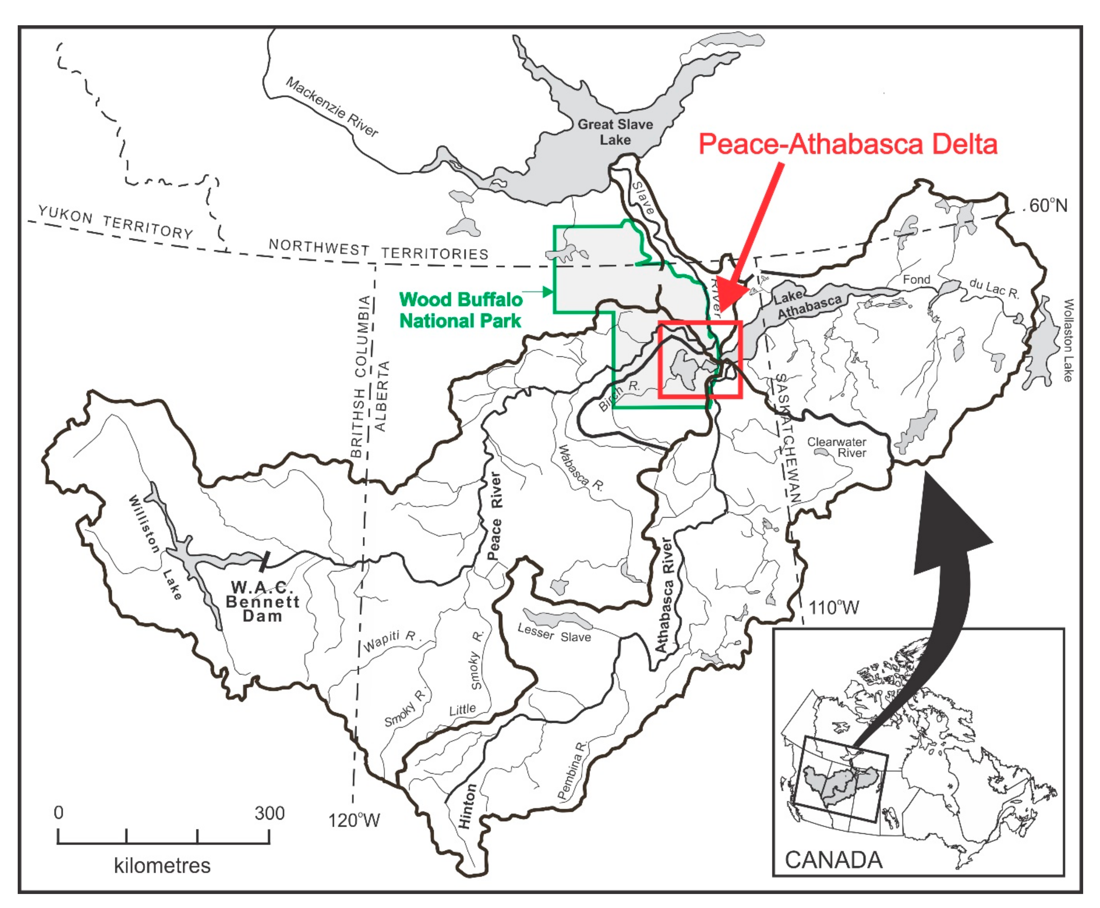
While much of the multisensor work to date has been on characterizing upland forest canopies, there has been little attention paid to characterizing wetland canopies/cover through the combination of active LiDAR and passive EO remotely sensed data. This paper will describe work that we have carried out in defining a framework for the processing and integration of LiDAR and satellite derived EO data to describe form. The utility of these various datasets is in their ability to provide us with a range of products which can describe a myriad of characteristics of geomorphologically and ecologically complex systems, such as deltaic ecosystems [51,52]. This paper reports on one aspect of work that is being carried out to characterize the ecology and hydrology of the Peace–Athabasca Delta (PAD) in northern Alberta (see Figure 1). We have focused on the use of readily available data (much of which is in the public domain) and open-sourced, freely available processing tools, such as R (https://www.r-project.org) for statistics and QGIS (https://qgis.org/) for visualization and spatial analysis.
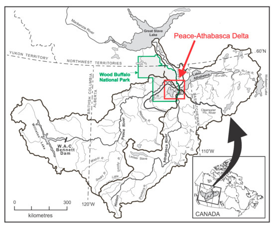
Figure 1.
Location of the Peace–Athabasca Delta (red rectangle) study area in northeastern Alberta, Canada.
2. Study Site
The Peace–Athabasca Delta (PAD) formed at the convergence of the Peace (~1680 km2), Athabasca (~1970 km2) and Birch (~170 km2) river deltas at the west end of Lake Athabasca in northwestern Canada [53] (Figure 1 and Figure 2). The PAD is a recognized wetland of international importance by the Ramsar Convention and 80% of the delta is protected within the Wood Buffalo National Park, a UNESCO World Heritage Site. In addition to extensive deltaic floodplain areas, the PAD complex (~6000 km2) encloses several large interconnected lakes. The study area of interest for this project is approximately 900 km2 that covers a large extent of the Athabasca Delta (white polygon in Figure 2).
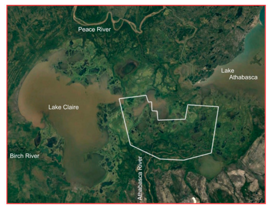
Figure 2.
Airborne LiDAR data acquisition area (white polygon) within the Peace–Athabasca Delta in September 2013. Basemap provided by GoogleEarth.
The river-lake-delta system drains Cordilleran and Boreal areas of approximately 600,000 km2 northwards towards the Slave River. During high water events on the lower Peace River resulting from ice jams and high flows, drainage may reverse southward into the central lakes, and in extreme events via overland pathways [54,55,56,57,58]. The Peace River has been regulated since 1968 by a number of dams, which control the headwater runoff for the generation of hydroelectricity, leading to important changes to the flow regime near and within the delta, which were partially remediated with the building of weirs on outflow channels [55,56,57]. The Athabasca River mainstem is unregulated, with <5% of the natural flow allocated for agriculture, municipal and industrial water uses and has, thus, retained a near natural hydrological regime [59]. Oil sanding mining (open pit and in situ) is occurring in tributaries of the Lower Athabasca River, upstream of the PAD, where landscape alterations and small amounts of water are abstracted from the mainstem for processing of bitumen [59,60].
The PAD contains more than 1000 inland wetland and lake basins with varying degrees of connectivity to the main flow system: open drainage, restricted and isolated basins [53,61]. The latter two classifications are commonly referred to as perched basins, which other than isolated areas with significant local runoff input (e.g., shield areas in northeast area of PAD), require periodic overland flooding during the spring breakup ice jams or summer high flows to offset loses of water in between inundation mainly through potential evapotranspiration being greater than precipitation (456 mm vs. 351 mm, respectively, historical mean 1985–2019) in the generally prevailing semi-arid climate [58,62]. This periodic flooding and water depth drawdown cycle produces variable, high biological productivity in these deltaic floodplain areas [51]. The sources of the water that contribute to particular wetlands is critical to ecosystem biodiversity. Wetland environments, which are developed from fluvial sources have levels of nutrients typically sufficient to promote a relatively broad diversity in terms of floral communities [63]. This range is in contrast to rainwater-sourced bogs, and groundwater fens, where the nutrient levels are lower, and the resulting vegetation is less varied and abundant. Additionally, those environments that are flooded periodically, rather than experiencing longer more sustained flooding, have options for a greater biodiversity [63].
The PAD has been recognized as a primary habitat for a large range of birds and mammals [51,64]. The 1982 Ramsar designation highlighted the PAD as an important wetland, based on its primary productivity and size, and is particularly important habitat for large ungulates, migratory birds, and fish. The vegetation cover, as reported on by Timoney [64], was affected by the frequency of flooding. Deciduous shrubs (Salix spp.) are sensitive to water levels and require hydric soil conditions to flourish, as do many of the graminoid species. Changes in the hydrological regime of the PAD due to flow regulation and climate change may therefore be producing changes in the health and distribution of the vegetation cover, and, by extension, to ecological services, due to changes in the frequency and magnitude of the flooding of delta areas adjacent to the stream courses [40]
Some of the early publications on the vegetation characteristics and distribution on the PAD were presented by Wickware [65] and Wickware and Howarth [66], Timoney [64,67,68], Timoney and Argus [69]. These publications noted that the distribution of vegetation was influenced by topography, as it dictated the frequency and duration of periodic inundations, and the depth to the ground water table. The vegetation succession in frequent short-duration flooding scenarios resulted in exposed mudflats to sedge meadows (Equisetum fluviatile and Equisetum palustre), to better drained herbaceous meadows through to willow (salix spp.). Areas which experience longer water residency times will have emergent macrophytes and cattails (Typha spp.) along the shorelines. The less frequently inundated areas are dominated by Carex spp. and Calamagrostis canadensis, followed by salix and alder (Alnus spp.). The time scale is typically up to 10 years from exposure to salix. In areas which are no longer inundated, especially areas leading up to the levees, and on scattered Precambrian metamorphic outcrops, salix is abundant followed by birch (Betula spp.), poplar (P. Tremuloides) and spruce (P. Glauca). In areas where the salix is well established it can achieve heights in excess of 6–7 m.
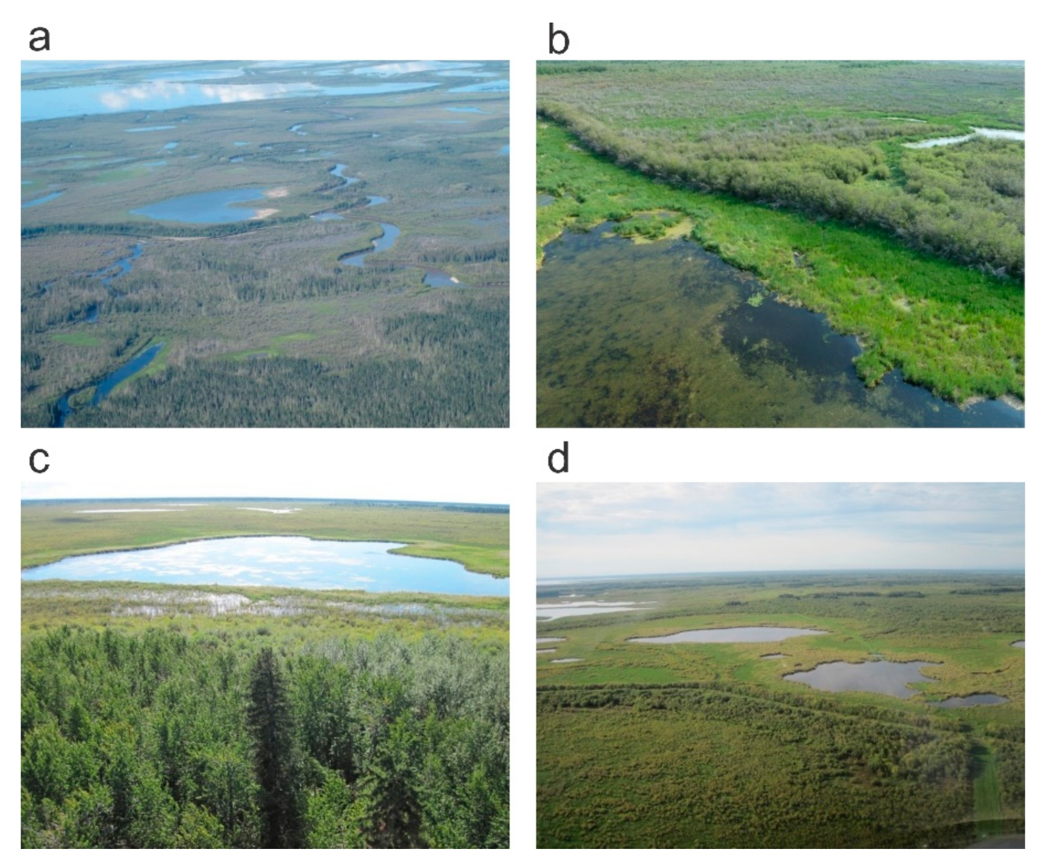
Examples of the vegetation complexes from the PAD area of interest are presented in Figure 3. Figure 3a represents a vegetation complex dominated by emergent vegetation, herbaceous meadows and (seasonally defoliated) deciduous willow stands. The topographically higher, older areas are characterized by deciduous–conifer stands. Figure 3b represents an area with standing water and emergent vegetation, and exposed emergent vegetation separated from the better drained herbaceous meadows/willow complexes by a low levee with dense willow stands. Figure 3c is another representation of an upland (conifer–deciduous) to water vegetation transition, including willows and emergent stands. Figure 3d is a view of an enclosed basin with some residual ponds but dominated by emergent vegetation/meadows. The enclosed levels support willow stands.
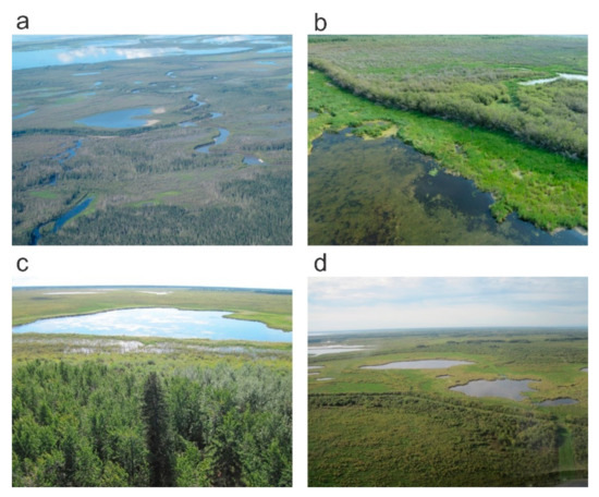
Figure 3.
Examples of wetland complexes within the study area of the Peace–Athabasca Delta: (a) Looking north over Johnny’s Cabin Pond, (b) Paired Lakes, (c) Embarras River, (d) Greywavies Lake. Photos taken by Environment and Climate Change Canada in August 2013.
3. Data and Processing
The data chosen for this study include those that are readily available, in most cases from open sources. These include EO data from the European Space Agency’s (ESA) Sentinel 2 (S-2) multispectral sensor, and airborne LiDAR data. While LiDAR data are strictly not open source, they are increasingly being made publicly available through government archiving. The Scandinavian countries have been forthcoming in providing freely available data, as have the individual US states. Canadian provincial and federal governments are also slowly providing these data as freely available to the public (e.g., Reference [70]).
3.1. Sentinel-2 Data
The S-2 data can be downloaded from the ESA data portal (https://scihub.copernicus.eu/dhus/#/home) as can an open source data processing package - SNAP (https://step.esa.int/main/download/snap-download/). SNAP allows the user to unpack the data and apply a number of processing procedures to derive a variety of products, including spatial resampling to a common pixel resolution, atmospheric corrections, and vegetation index derivation for a number of common indices. It will also output the data into a number of non-proprietary formats. The spectral bandset and associated spatial resolutions of the S-2 multispectral imager (MSI) data is summarized in Table 1. The S-2 constellation is composed of two separate satellites with nearly identical band configurations. S-2A was launched in June 2015 and S-2B in March 2017. Both are in a sun-synchronous orbit separated by 180°, imaging at ca. 10:30 mean local solar time (MLST), which is similar to other EO platforms (e.g., LANDSAT and SPOT), so that the data and results are comparable. The orbital configuration of the two platforms, and relatively wide scan swath, yields a high frequency revisit time of ca. 5 days.

Table 1.
Spectral Characteristics of Sentinel-2 (S-2) Multispectral Imager (MSI).
For the classification portion of the project we chose a scene from the S-2B platform acquired on 19 September 2019. The chosen data were processed by ESA to a level 1C Top of Atmosphere (ToA) reflectance, and orthorectified—projected to a WGS 84 geodetic reference system, subsequently re-projected to a Universal Transverse Mercator (UTM) reference grid for further data processing.
3.2. Sentinel Data Processing
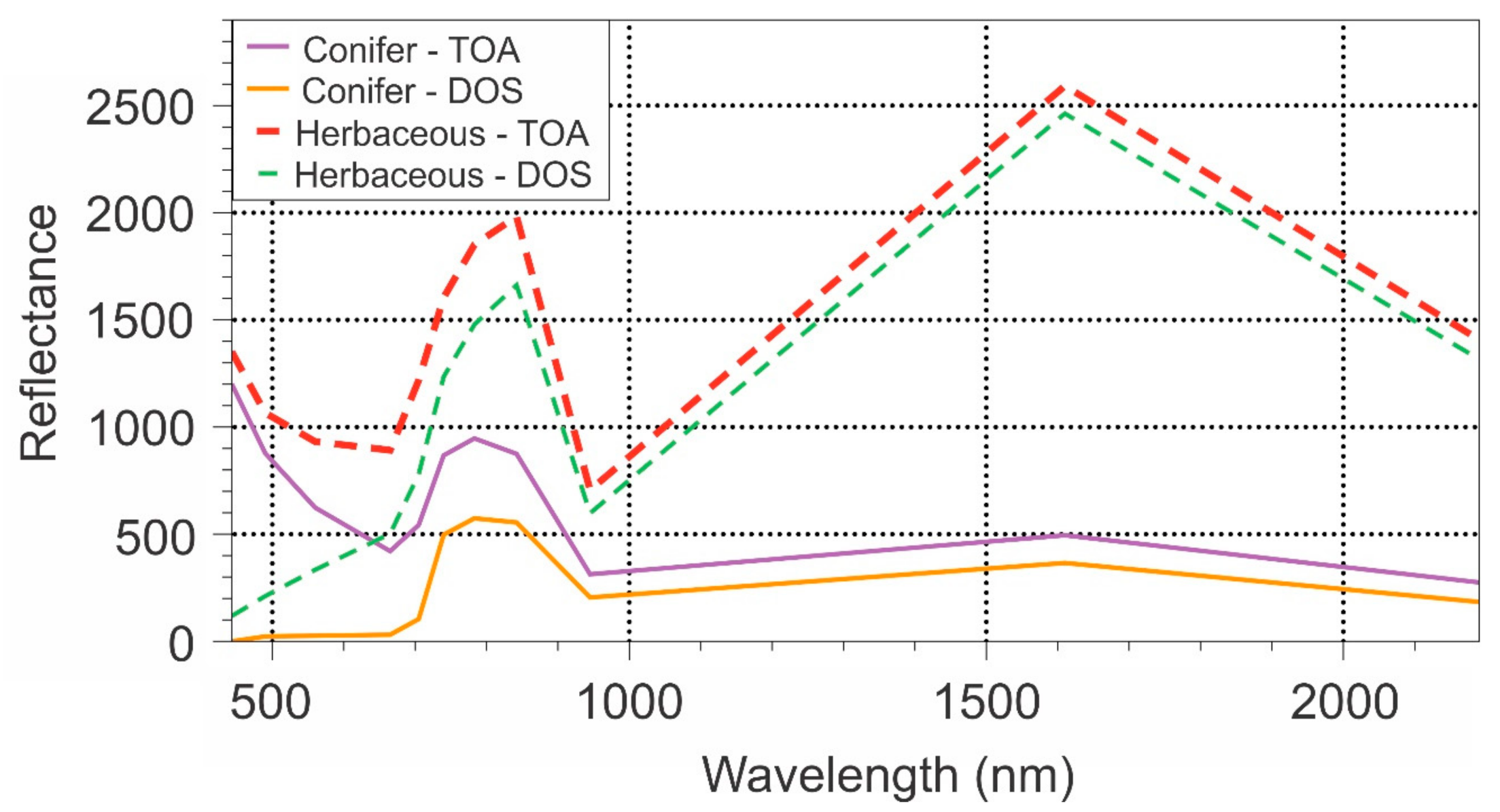
The S-2 data were unpacked and spatially resampled to a consistent 20 m grid size for all bands using the SNAP toolbox. The S-2 bands with 60 m grid cells were resampled using a nearest neighbor approach. The 10 m bands were coarsened using a bilinear convolution resampling strategy, employing a distance decay interpolation approach to derive the coarser pixel value. Level 1C S-2 data was converted to ToA reflectance, where the recorded upwelling radiance was normalized based on downwelling solar irradiance. The resulting data does not account for atmospheric attenuation and path radiance issues. Normally, we would use calibrated ground reflectors and an empirical line correction (ELC) to remove these effects. Unfortunately, we did not have access to spectrally stable targets representing bright and dark reflectors that were suitable for this purpose. We therefore had to rely on a dark object subtraction (DOS) to estimate path radiance, and mitigate its effects. We recognize that DOS is not the ideal approach to solve for atmospheric effects, however given the proximity of substantial water bodies to the terrestrial surface we felt that it was important to reduce the effects of water vapor, especially with the shorter wavelengths. For this we located deep water, assuming that its reflectance would be negligible, as the dark object and subtracted the measured water values (the difference is assumed to be caused by path radiance) from the remainder of the pixels in that band. The representative S-2 spectra (presented in Figure 4) yield patterns that are consistent with ground reflectance spectra. We can see that the effects of the atmosphere are preferentially focused on the shorter wavelengths with less effect in the infrared.
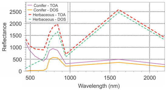
Figure 4.
Effect of dark object subtraction (DOS) on Sentinel-2 reflectance spectra for selected cover types. TOA is top of atmosphere reflectance.
The S-2 data were classified to assign cover types to the individual pixels. We adopted two approaches to classify these data, each one yielding different, but related, outcomes. The first was a more classical classification approach utilizing a nonparametric spectral angle mapper (SAM) classifier [71]. This supervised classifier uses a spectrum shape-based approach to assign class labels to the individual pixels. The approach allows us to define cover types based on spectral libraries that allow for slight variations in shape. Its advantage is that the classifier is unaffected by intensity variations as it focuses on shape, so our use of a dark-object adjusted TOA reflectance is appropriate. The implementation of the SAM classifier used here can be found in the RSToolbox package in R. A spectral library was built based on samples chosen from a high resolution (2 m) RGB reference image. This library was comprised of 86 spectra representing deciduous, coniferous, herbaceous, emergent vegetation, open soil, turbid water, and clear water.
One drawback using a standard classification approach is that each pixel is assigned a unique class, even though there is a mixture of classes within the area represented by the pixel (in this case 400 m2 in a 20 m pixel). A second classification approach was therefore adopted which uses spectral mixing analysis (SMA) to decompose each pixel into an approximation of the proportional contribution of each cover class. The SMA approach uses a series of spectral endmembers that define “pure” reflectors within the image. These form the basis of the unmixing, where unknown mixed spectra are compared to the pure endmembers, and the proportional contribution of each endmember is determined. The result is an output image file that contains the estimated contribution of each class to the pixel. With this approach, we are presented with the possibility of assessing the contribution of each cover class to each pixel. The assumption adopted for this analysis is that each reflector contributes proportionately in a linear fashion, and that the solution is constrained from 0 to 1, so that a summation of the layers at each pixel location does not exceed 1.0.
To assess the accuracy of the initial classification we relied on 0.30 m aerial photography obtained during the LiDAR aerial survey, as well as ground photography during ecological monitoring campaign. We generated a network of randomly selected points that we interpreted into the basic classes defined above. While there may have been some misinterpretation of the vegetation occurring at these points, if was felt that the class labels that we were defining were sufficiently broad that this source of error was not deemed to be significant.
3.3. LiDAR
LiDAR data were collected over the area of interest in September 2013 over a period of three days (see Figure 2) using a Reigl 780 laser, mounted in a twin-engine Navaho aircraft. The point repetition frequency was 240 KHz at a flying height of 1500 above ground level (AGL). That resulted in an average point density of 10 points per m2. The laser is a waveform system, operating at a 1064 nm wavelength, where the data can be extracted as discrete multiple returns (in this case first, last and 2 intermediate). This longer wavelength reduces the atmospheric influences caused by water vapor. The resulting point cloud was parsed into 1 km2. blocks for further processing. Ground control was located at the nearby Fort Chipewyan Airport.
3.4. LiDAR Data Processing
The LiDAR point cloud was calibrated and classified by the data surveyor (Terra Remote Sensing Inc.). Calibration positions the data in absolute 3-D space in co-ordination with a ground base station. Further, pre-calibration work, also removed spurious air hits, from atmospheric noise (not likely with the longer wavelength laser) and birds. The classification processing consisted of separating ground hits from those interacting with vegetation. The resulting point cloud was separated to yield a class with exclusively ground points and a second class with vegetation points only. A terrain-normalized canopy height model (CHM) of the vegetation point cloud was produced for further processing and analysis along with the ground points.
The ground point cloud was gridded to a 2 m grid to yield a digital elevation model (DEM). This DEM was further processed to generate derivative products. These products included, the first partial derivative-slope gradient, and the direction of the maximum slope—i.e., aspect, and the second partial derivative—curvature, in both the upslope and cross slope directions. In addition, we derived a topographic wetness index (TWI) [72,73]:
where a is the upslope drainage area, and b is the slope gradient. These metrics were upscaled to a 20 m grid resolution to coincide with the S-2 data, by using the average of the 100 two-meter values within the larger grid cell. Another derived metric was Rugosity, or surface roughness, which was the standard deviation of heights within the 20 m grid cell [74].
The vegetation classed point cloud was first terrain-normalized to remove elevation effects. We derived descriptive metrics that characterize the vertical and horizontal 3-D structure of the canopy within a specified 20 m grid cell using the CHM point cloud. The process by which this is done has been fully described in the literature [75,76]. This process has been extensively applied to forested environments, including Boreal forests. Initially we organized the points within each 20 m grid cell in quantiles—Lhq (5, 10, 15, …, 100). All vegetation points with a height greater than 1 m were considered. This value was chosen to minimize the effect of noise from ground clutter. Second, we adopted the use of L-moments to describe the vertical distribution of the point cloud within the grid cells [77]. We used L-moments, rather than product statistical moments, as they are more robust and less effected by outliers [78]. We addressed the gap structure of within the grid cell through the determination of the canopy gap fraction (CGF);
where n is the number of first returns above a specified height, and N is the total number of first returns for the grid cell. Using this approach, we derived a single CGF for the grid cell above the 1 m lower height cutoff, or in combination with the Lhq we can derive a vertical distribution of the canopy within the grid cell. We also extracted the Co-dominant canopy height, or the height of the 85th percentile in the grid cell, and Skewness, which describes whether the point cloud is biased towards the top (negative) or the bottom (positive) of the distribution.
3.5. Statistical Analysis
The statistical analysis used in this work centered on the use of nonparametric methods. As mentioned above the initial classification of the S-2 data utilized a SAM and subsequently a SMA to expand the characterization of the cover classes. To explore the relationship of the S-2 classes and the LiDAR metrics, we employed an unsupervised data mining - cluster analysis. For this procedure, we used K-means clustering as implemented in R, where the input variables were normalized so as to standardize the scales of the distributions, and to reduce the dominance of the variables with the larger values. The data were initially standardized so as to remove biases introduced by input variables having different scaled distributions. We employed the Silhouette method [79] to determine the optimum number of clusters of the samples to be clustered. Finally, we used a Kruskal–Wallis test to explore whether the resulting clusters represented distributions that were significantly different from each other.
4. Results and Discussion
Initial work to map the distribution of various vegetation/ecological complexes in the PAD was presented by the PAD-PG [53] based on 1970 air photos. With the advent of EO in the 1970s, Wickware [65], Wickware and Howarth [66], Jaques [80], and Töyrä and Pietroniro [40] provided updated maps. Wickware and Howarth [66] found that given the coarse spatial resolution of the original LANDSAT data, as well as the relatively low number of broad spectral bands, their ability to characterize the vegetation communities in any detail was challenging. Töyrä and Pietroniro [40] working with LANDSAT Thematic Mapper data (30 m spatial resolution), and its enhanced spectral band set over the original LANDSAT data, RADARSAT C-band microwave data, and a detailed LiDAR-derived DEM, were also unable to expand significantly on the cover classes that could be resolved in prior work. They did however through the use of the DEM delineate areas which had a more frequent and longer-lasting flood inundation.
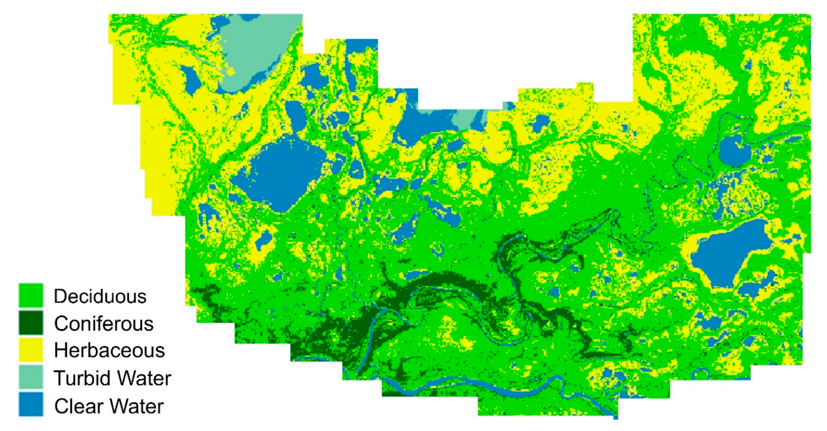
Our initial classification of the S-2 data using the SAM approach is presented in Figure 5, with the accuracy for the main vegetation cover types in Table 2. The accuracy assessment was carried out using aerial photographs as the interpreted “truth”. As can be seen, the classification was simplified somewhat to collapse the herbaceous meadows with the emergent vegetation as they were highly confused. Many of the areas normally flooded in the spring/early summer and where the herbaceous vegetation would be considered to be emergent, were dry at the time of the image, and so the vegetation appeared similar spectrally to meadows. For this portion of the work we thus merged the two classes. The overall accuracy for the terrestrial classes considered is high (82%), with a Cohen Kappa Coefficient [81] of 0.72, which indicates a strong confidence in the quality of the classification.

Figure 5.
Spectral angle mapper (SAM)-based classification derived from the Sentinel-2 imagery.

Table 2.
Classification Confusion Matrix for Main Cover Types.
The two water classes (deep water and turbid water) were not included in the accuracy assessment as (i) water generally tends to have relatively high accuracies, potentially distorting the accuracies of the more problematic terrestrial classes, and (ii) the turbid water class is transient, likely leading to inconsistencies with other image sources acquired at different times. Some of the terrestrial misclassification comes from confusion of the S-2 based classification that is between conifer and deciduous. This can, in part, be explained by the fact that given a low sun angle at this latitude in September would have affected some of the deciduous pixels, especially where the canopy was open. In spite of the relatively high classification accuracy, the relatively simple classification scheme produced by passive optical data and a traditional classification algorithm does highlight the limitations of these types of data.
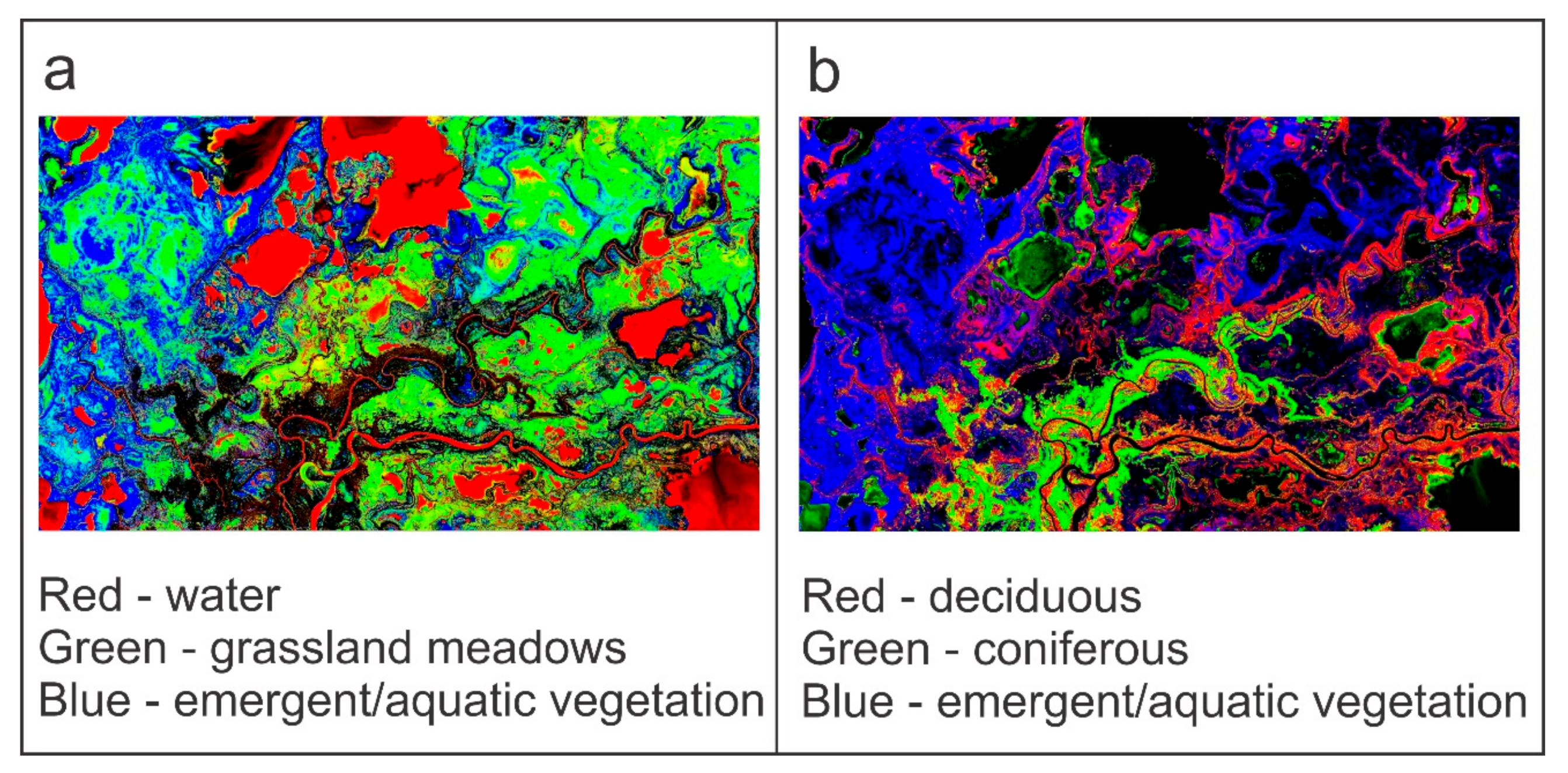
To overcome the limitations detailed in earlier works and in this current study, we expanded our classification of the SMA. Examples of the output projected through RGB channels are presented in Figure 6. There are a number of problems with this product as well, related to the same issues that we experienced with the SAM classification above. There is the problem with an over estimation of conifer especially along the shorelines as well in the waterbodies themselves. These areas are represented by pixels whose mixtures yield a spectrum shape that is more similar to that of conifer than herbaceous or deciduous spectra.
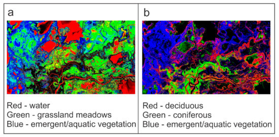
Figure 6.
Output examples from the spectral mixing analysis (SMA) projected through red-green-blue (RGB) channels. The classes are separated into the two images (a,b) to provide us with an opportunity to view the per pixel class distributions as continuous, rather than as discrete classes.
A comparison of the SAM and SMA derived classifications is difficult. However, we sampled the two classifications produced in this work and compared the SAM-derived class to the class label representing the maximum cover type defined by the SMA for the corresponding pixel. Based on this approach, the overall correspondence between the two classifications is 73% (Table 3) with a Kappa of 0.60. However, it must be kept in mind that in many cases the mixtures were quite complex and that while the maximum may not correspond, the percentages may be close, and the comparison will underestimate the correspondence of the two. The relatively high degree of confusion between the deciduous and herbaceous/emergent classes occurs mainly in the topographically lower areas where sufficient moisture may delay the onset of senescence, resulting in the grasses there reflecting similarly to deciduous areas.

Table 3.
Confusion Matrix between the Spectral Mixture Analysis (SMA) and Spectral Angle Mapper (SAM) based classifications.
The LiDAR canopy and landscape metrics used in this study are presented in Figure 7 and Figure 8. Two metrics characterize the vertical structure (co-dominant canopy height and skewness) and two metrics the horizontal structure (CGF and rugosity). The CGF describes the gaps that extend to the canopy floor (1 m), while the rugosity addresses the “bumpiness” of the top of the canopy. The co-dominant height was used, so as not to report on the absolute highest value in the 20 m grid cell, but rather the top of the co-dominant canopy. The skewness of the point cloud is a metric that embodies a complex interpretation. It was also noted that many of the areas that were classified as emergent vegetation have heights below 1 m, and are thus deemed to have a height of 0. Taller deciduous canopies such as poplars will have canopies concentrated towards the top of the distribution (negative skewness), as they are self-pruning, while willows are not and will be more uniformly distributed. In a transect which is increasingly hydric, the separation of the larger stems will increase, and the point cloud will become more dominated by understory vegetation returns, leading to increasingly positive skewness.
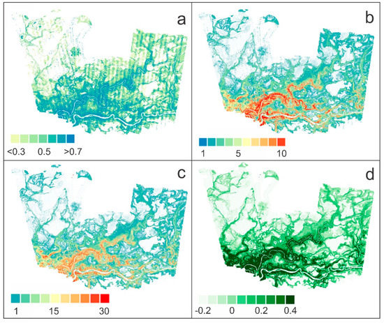
Figure 7.
Canopy metrics derived from LiDAR canopy height model (CHM) point cloud: (a) canopy gap fraction (%), (b) Rugosity (m), (c) Co-dominant height (m), and (d) Skewness (unitless)–negative values represent a top-loaded distribution, positive numbers represent a bottom-loaded distribution.
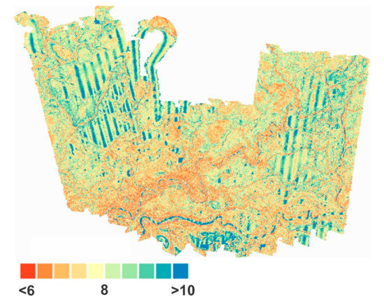
Figure 8.
Topographic wetness index (TWI). Banding caused by a combination of very low LiDAR height values and a slight “cupping” of the data at the edges of the flight lines. These areas are typically associated with waterbodies and so would be masked out during prior to analysis. Lower values represent positions that are relatively topographically higher in the landscape.
We chose to use the TWI to represent the topographic effects of the landscape as it is a metric incorporating the upslope drainage area along with the local gradient, which addresses a global measure of contribution area with the ability of local landscape to shed moisture. The PAD region of interest that we are looking at is one with relatively little relief and topographic variation. Small differences in topography have profound effects on the distribution of moisture and the landscape’s ability to shed it. What we can observe from Figure 8 is that the areas with the lowest TWI values correspond to the topographically higher portions of the delta landscape, which correspond to the older portions of the area represented by levees. The TWI does provide us with a method to quantitatively characterize the areas of topographically-defined receiving areas for water within the landscape. Given the low topographic variability, and the relatively coarse size of the study grid cell at 20 m, however, the sensitivity of the index maybe questionable.
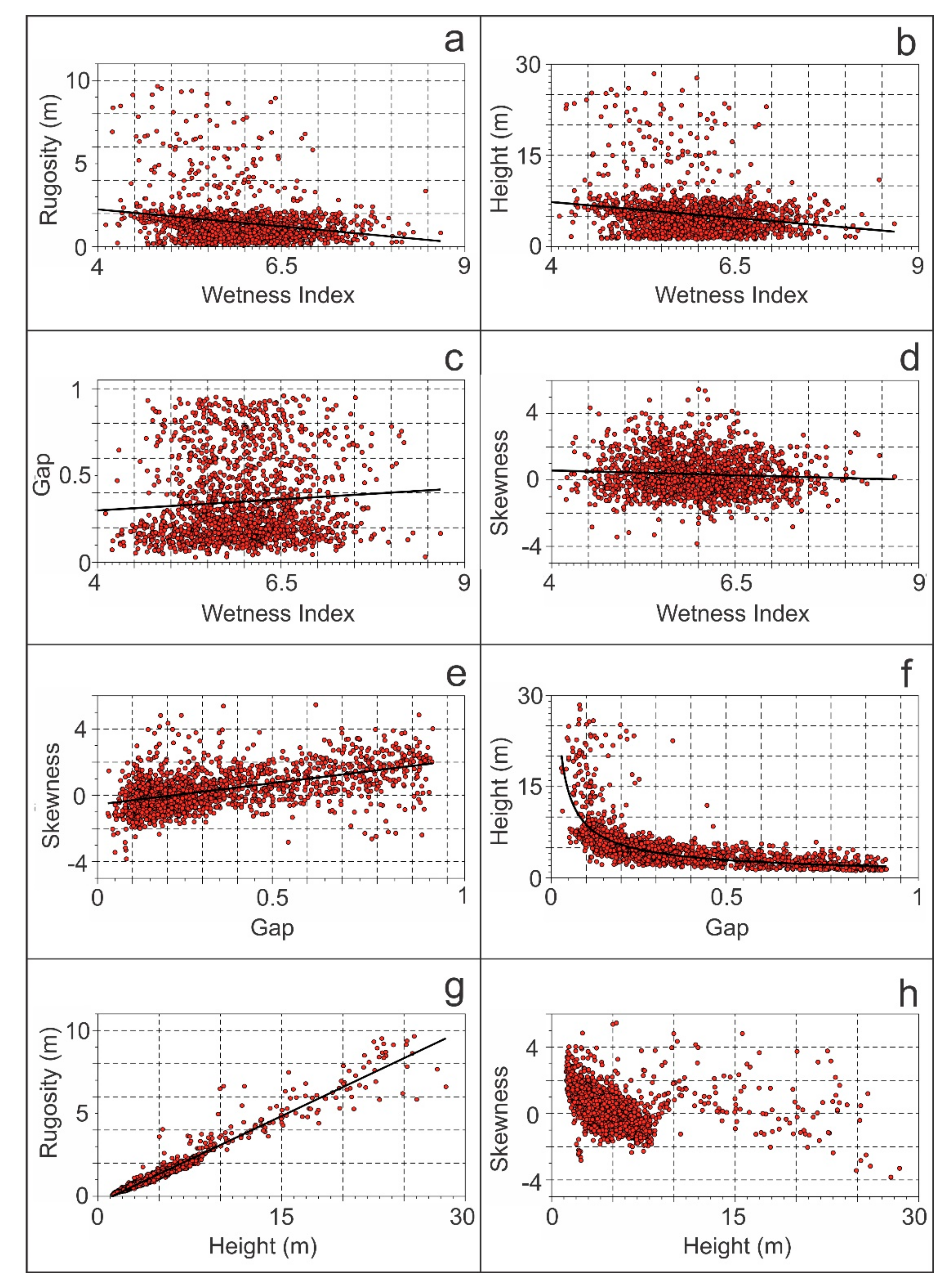
The output from the SMA and LiDAR metrics (canopy and TWI) were sampled using a random sample design of 3000 points. Figure 9 reveals bivariate relationships between the individual canopy metrics. There is a general decrease in the overall height and rugosity of the canopy with increases in TWI. Additionally, the rugosity and height are closely correlated. The relationship between the TWI and CGF and skewness is less well defined, to the point where the two-canopy metrics appear to be insensitive to changes in TWI. This might well be related to the influence of the periodic flooding caused by overbank infill of depressions from high flow or ice jam, events and not through landscape-related drainage and flow. The CGF remains fairly stable with changes in the canopy height down to a break at the 8–10 m point, after which the gap fraction increases rapidly with relatively minor changes in height. The skewness-height relationship yields an interesting pattern. There is a well-structured pattern in the lower canopy (<8 m), where there is a rapid shift in the point cloud distribution towards the top of the canopy. After the 8 m break the pattern is repeated. This 8 m break might very well represent the break between the “upland” vegetation types (trees) and the wetland types (shrubs and grasses). Finally, the relationship between the skewness and CGF is straight forward, and behaves as expected, with a lowering of the point cloud as the gap fraction increases.
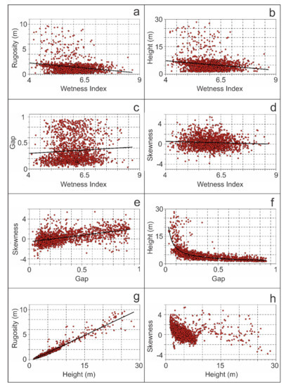
Figure 9.
Relationship between LiDAR metrics: (a) Rugosity, (b) Height, (c) Gap and (d) Skewness versus Wetness Index; (e) Skewness and (f) Height versus Gap; (g,h) Rugosity and Skewness versus Height.
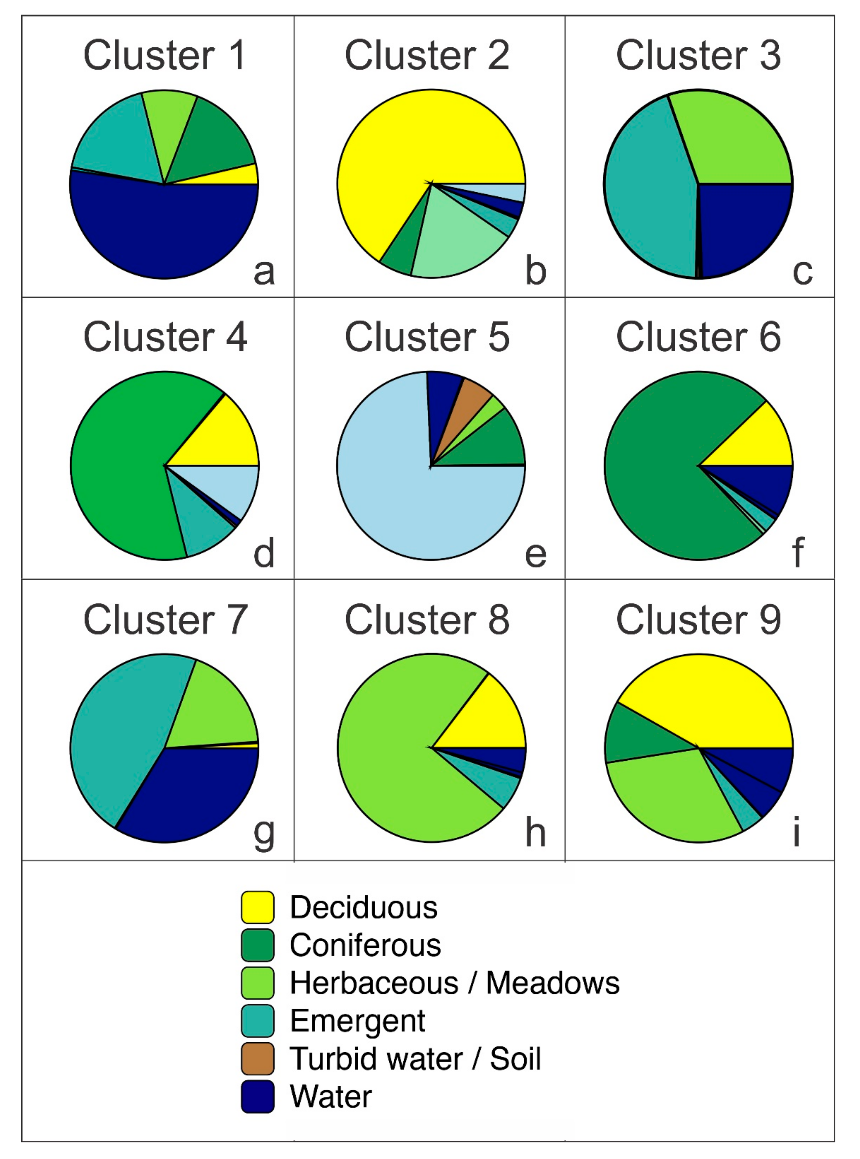
To address the relationships between the classified cover types and the LiDAR metrics we adopted a K-mean cluster analysis and Silhouette method [79], which gave us two candidate number of clusters (six and nine). Although the strongest case could be made for six clusters, we implemented our clustering with nine clusters, as this allows us to collapse clusters, we judge too close to be meaningfully different. The summary of the cover types found within each of the cluster is presented in Figure 10. Cluster 5 is represented by a majority of deep and turbid water classified pixels with a small number of other classes including herbaceous and conifer. The conifer classed pixels in this cluster can be attributed to edge mixtures which produce a conifer-like spectrum. Cluster 1, with its complex mixture, was interpreted as being emergent vegetation with a significant water component. Clusters 3, 4, and 7 with less complex diversity are also interpreted as emergent vegetation classes.

Figure 10.
Summary of landscape cover classes within each cluster (1–9, (a–i) respectively).
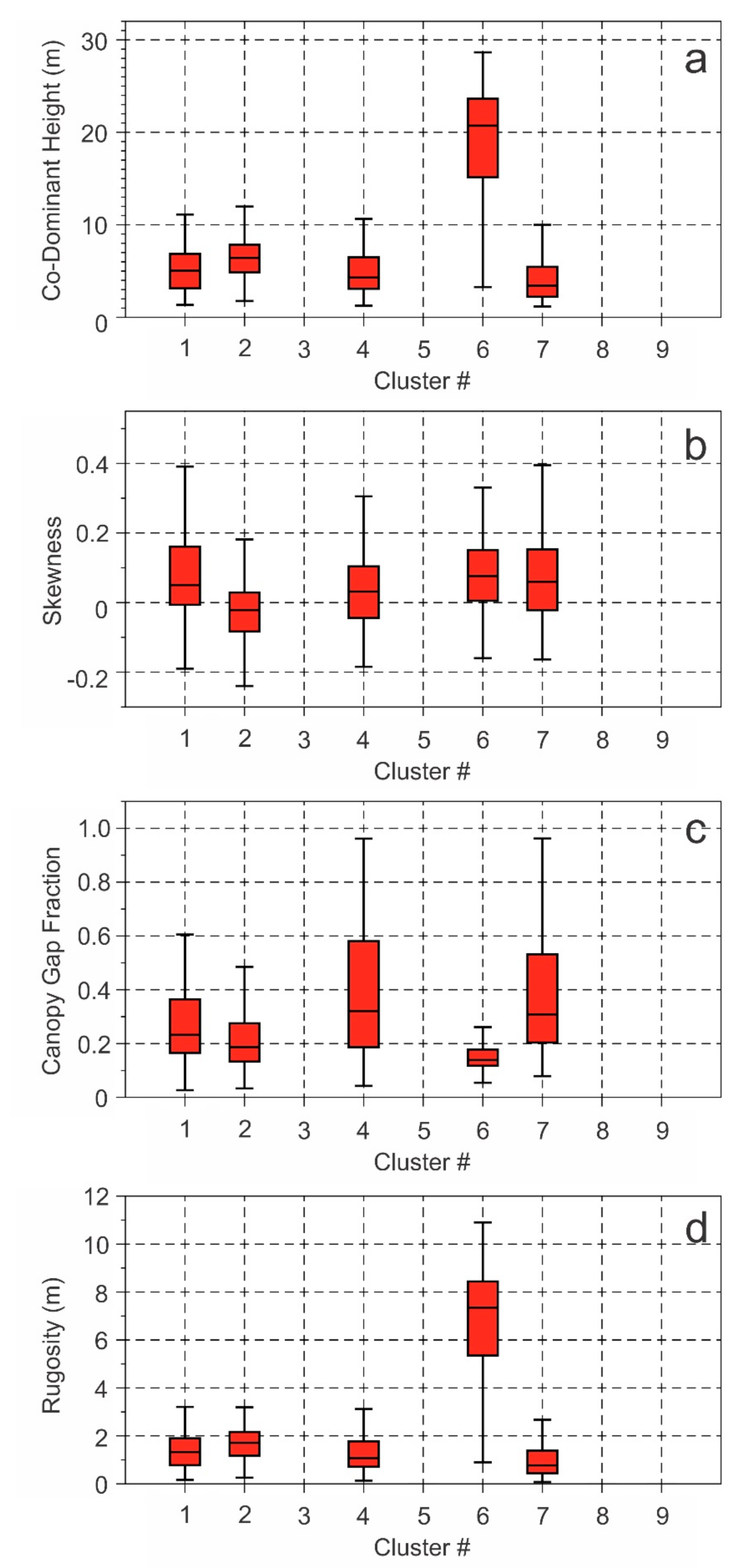
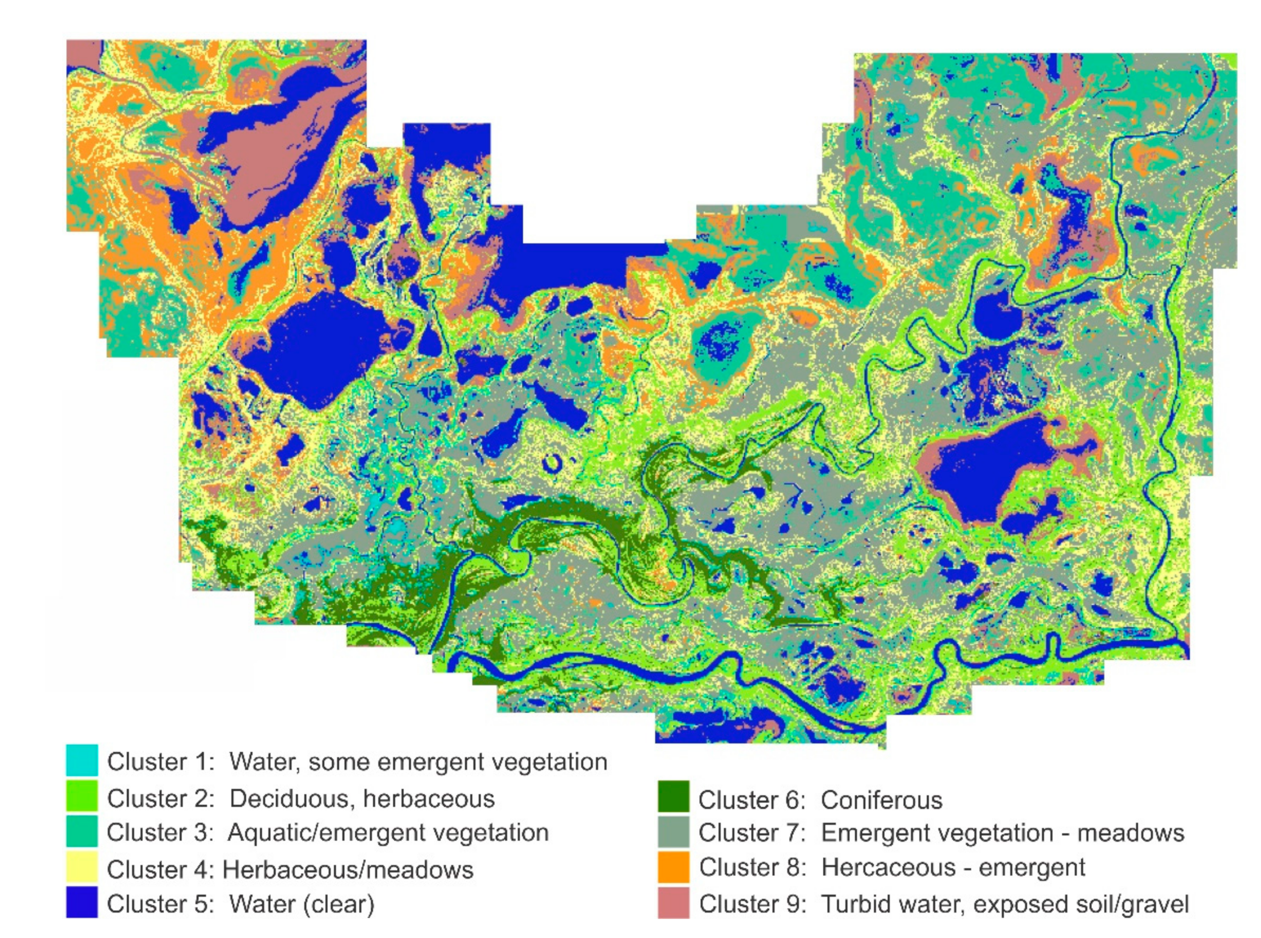
When we examine the LiDAR canopy metrics (Figure 11) and TWI (Figure 12) in relation to the cover classes, a more refined interpretation of the class structure can be assigned. The final cluster map is presented in Figure 13. The classification in Figure 13 is a refinement of the earlier SMA-based one, and does not represent an entirely new segmentation of the image. The LiDAR metrics generated in this work are statistical summaries of the point cloud for that specific pixel area, and their inclusion does not change the initial classification but rather adds additional information. As such the accuracy of this classification product can be viewed as being consistent with the earlier SMA-based one as summarized in Table 3.
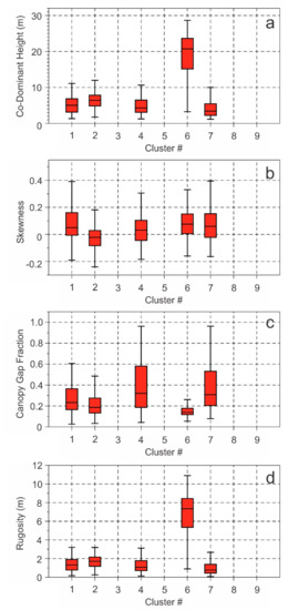
Figure 11.
Summary of LiDAR vegetation metrics for cluster 1 through 9: (a) Co-dominant Height, (b) Skewness, (c) canopy gap fraction, and (d) Rugosity.
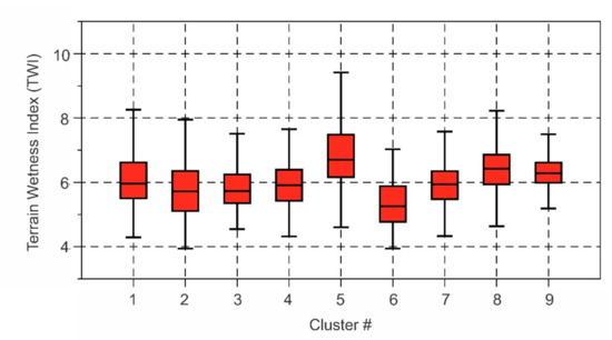
Figure 12.
Summary of terrain wetness index (TWI) by cluster.
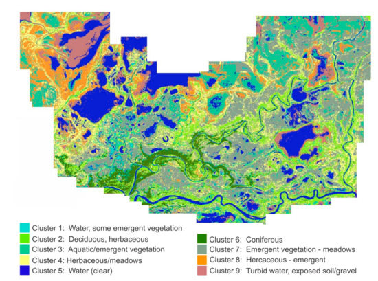
Figure 13.
Spatial representation of cluster analysis.
Cluster 1 which was interpreted as being emergent vegetation dominant can be further qualified with the LiDAR data. We can see by the canopy heights that the average is just under 5 m, and that the gap fraction is low. This would be indicative of pixels which are close to the shoreline so as so have a riparian component. Additionally, many of the emergent grasses, such as cat tails, extend in dense thickets above the water surface, so this is completely consistent. Cluster 2 is predominantly deciduous with a significant herbaceous component. The height range is from 2 to 13 m with an average of 7 m, while the skewness is the lowest of all of the classes and the gap fraction remains low, indicating an increasing top loading of the canopy. Finally, we can see that this cluster is spatially distributed primarily along the river courses. This would correspond to the balsam poplar stands, and to a lesser extent some of the taller willows transitioning to the more mature poplar areas.
Clusters 3 and 4 might be interpreted similarly with only the optical results available, however when we consider the LiDAR canopy metrics as well, the interpretation diverges. Cluster 3 is primarily herbaceous with a significant component of water, with the LiDAR data indicating that all of the vegetation found within this cluster is lower than 1 m. Cluster 4 on the other hand has an average height of 5 m, with a range from 1 to 10 m, a moderate skewness and a large range in CGF. Cluster 5 has no LiDAR canopy points above 1 m and so can confidently be labeled as water, even though there is a small proportion of grass and conifer edge pixels. Cluster 6 has been designated as the one representing conifers. The cover classes encapsulated in this cluster are primarily conifer, with a small proportion of deciduous and herbaceous. There are also some water dominant pixels in this class, although they have been interpreted as mixed or edge pixels. Cluster 7 is primarily herbaceous with a significant proportion water, similar to Cluster 3. The canopy metrics however differ from Cluster 3 in that average height is approximately 3 to 4 m, with a corresponding low rugosity, the skewness suggests that the canopy is loaded towards the ground, and that the CGF range is high. This suggests that this cluster represents environments that are close to water body edges where hydration promotes stands of cattails, etc.
The spatial representation of the clusters (Figure 13), however, suggests that Cluster 3 lies spatially between open water and Cluster 7. The same can be said for the difference between Clusters 4 and 8, where Cluster 8 is more proximal to the current water bodies while Cluster 4 is situated further removed. The final cluster, Cluster 9, has a canopy below 1 m, but has a mixture of cover classes composing it. When examining the spatial distribution of this we see that it is a mixture of turbid water and exposed soil or sediment. Some edge pixels will have some vegetation so there are some inclusions of deciduous and herbaceous cover.
A Kruskal–Wallis test to assess the difference between median values was performed to quantify the interpretation of the graphical presentation in Figure 11. Prior to this we performed a Shapiro–Wilk test to assess the assumption of normality. The samples showed a significant deviation from normal distribution, so a non-parametric ANOVA (that is the Kruskal–Wallis test) was used here. As can be seen in Table 4, there is a statistical difference between the medians of most of the clusters with regard to the canopy metrics. Clusters 2 and 4 are not substantially different with regards to height and rugosity, while Clusters 4 and 7 have similar Gap Fractions, and 1, 6, and 7 have similar Skewness values. This provides further strength to the interpretations for the ecosystem characterizations above.

Table 4.
Results for Kruskal–Wallis pair-wise comparisons.
As described earlier, the TWI had a low range given the relatively low relief and small drainage areas (Figure 12). We can see that the between cluster ranges are slight with the Cluster 5 having the highest values, but since all of the bodies of water did not occur at the lower portions of the landscape and the other clusters being scattered around the area, it is meaningless to attempt to ascribe a statistical characterization. The Kruskal–Wallis test for the TWI (Table 4) provides some clarity as to the behavior of this index relative to the observed clusters. Clusters 1, 2, and 3 occupy similar landscape positions and so would be expected to have similar TWI. The proximity of some of the relatively younger deltaic stream channels where much of the vegetation would be deciduous (willow) with the wetland ponding areas would account for the similarity in TWI distributions.
5. Conclusions and Future Considerations
Integrating the passive optical and active LiDAR data provides us with an opportunity to explore both the form and functioning of a complex, low relief, deltaic wetland environment. It also provides a framework for monitoring and assessing long-term cumulative effects from climate change, flow regulation and oil sand mining in the PAD region. The main output from this analysis is a spatial representation of ecosystem vegetation structure both in terms of broad vegetation classes and their 3-D structures. While the broad spatial patterns coincide with the mapping that has previously been published for the area, the level of detail that can be extracted is substantially higher given the higher dimensionality of the input data.
A number of advantages can be realized from this product as an output for further analysis. It provides a foundation, or template, for further analysis, so that we can now address some of the spectral response both radiometrically and spatially that are partitioned to various ecosystems, rather than examining them on a more global (relative to the study area) basis. This will form the basis of the next analytical phase which will investigate the intra- and interannual changes in the ecosystem form and functioning of the delta wetlands as demonstrated by the changes in S2-derived LAI, fPAR, and vegetation indices.
For this work we have focused on S-2 MSI data. There are a number of other EO platforms, however, that provide us with a temporal dataset that the S-2 at this time does not. The LANDSAT program has a continuous data archive that extends back to 1972, although the current Thematic Mapper, and earlier, instruments extend back to 1986. The more limited band set on the LANDSAT series of satellites, however, reduces the definition of the spectrum, and so will limit the classification efficacy.
Author Contributions
Conceptualization, D.L.P., K.O.N., R.S.; Methodology, K.O.N., D.L.P., R.S.; Software, K.O.N., D.L.P., R.S.; Validation, K.O.N., D.L.P., R.S.; Formal Analysis, K.O.N., D.L.P., R.S.; Investigation, D.L.P., K.O.N., R.S.; Resources, D.L.P., K.O.N., R.S.; Data Curation, D.L.P., K.O.N., R.S.; Writing—Original Draft Preparation, D.L.P., K.O.N., R.S.; Writing—Review and Editing, D.L.P., K.O.N., R.S.; Visualization, D.L.P., K.O.N., R.S.; Supervision, D.L.P., K.O.N.; Project Administration, D.L.P., K.O.N.; Funding Acquisition, D.L.P., K.O.N. All authors have read and agreed to the published version of the manuscript.
Funding
This work was funded by Environment and Climate Change Canada (ECCC), LookNorth, and the Oil Sands Monitoring (OSM) Program. This work is contribution to the OSM Program but does not necessarily reflect the position of the Program.
Acknowledgments
This work was initiated and supported by Environment and Climate Change Canada (ECCC) through several programs and projects: Oil Sands Monitoring (OSM) Program “Acquisition of Aerial High Resolution Digital Ground Terrain Information in the Peace Athabasca Delta” and “Design of a Deltaic Wetland Ecosystem Health Monitoring” Projects; Climate Change and Adaptation (CCA) Program; ECCC Grants & Contributions to the University of Victoria; LookNorth Funding to Terra Remote Sensing Inc that conducted the aerial surveys. This work was partially funded under the OSM Program and is a contribution to the Program but does not necessarily reflect the position of the Program.
Conflicts of Interest
The authors declare no conflict of interest.
References
- Environmental Protection Agency Wetlands. Available online: https://www.epa.gov/wetlands/why-are-wetlands-important (accessed on 15 September 2020).
- Ducks Unlimited Wetlands. Available online: https://www.ducks.ca/our-work/wetlands/ (accessed on 15 September 2020).
- Nature Conservancy Canada All about Wetlands. Available online: https://www.natureconservancy.ca/en/blog/archive/all-about-wetlands.html#.XaobTEnsaUk (accessed on 15 September 2020).
- Ramsar Homepage. Available online: https://www.ramsar.org/ (accessed on 29 August 2020).
- Malty, E.; Baker, T. The Wetlands Handbook; Blackwell Publishing Ltd.: Hoboken, NJ, USA, 2009; ISBN 978-0-632-05255-4. [Google Scholar]
- National Wetlands Working Group (NWWG). The Canadian Wetland Classification System, 2nd ed.; Warner, B.G., Rubec, C.D.A., Eds.; Wetlands Research Centre, University of Waterloo: Waterloo, ON, Canada, 1997. [Google Scholar]
- Federal Geographic Data Committee Classification of Wetlands and Deepwater Habitats of the United States. Wetlands Subcommittee. Available online: https://www.fgdc.gov/ (accessed on 15 September 2020).
- Schindler, D. Sustaining Aquatic Ecosystems in Boreal Regions. Conserv. Ecol. 1998, 2. [Google Scholar] [CrossRef]
- Lomnicky, G.A.; Herlihy, A.T.; Kaufmann, P.R. Quantifying the extent of human disturbance activities and anthropogenic stressors in wetlands across the conterminous United States: Results from the National Wetland Condition Assessment. Environ. Monit. Assess. 2019, 191, 324. [Google Scholar] [CrossRef]
- Davidson, N.C. Wetland Losses and the Status of Wetland-Dependent Species. In The Wetland Book: II: Distribution, Description and Conservation; Finlayson, C.M., Milton, G.R., Prentice, R.C., Davidson, N.C., Eds.; Springer: Dordrecht, The Netherlands, 2016; pp. 1–14. ISBN 978-94-007-6173-5. [Google Scholar]
- Bergkamp, G.; McCartney, M.; Dugan, P.; McNeely, J.A.; Acreman, M. Dams, Ecosystem Functions and Environmental Restoration: Final Version; World Commission on Dams: Cape Town, South Africa, 2000. [Google Scholar]
- Rooney, R.C.; Bayley, S.E.; Schindler, D.W. Oil sands mining and reclamation cause massive loss of peatland and stored carbon. Proc. Natl. Acad. Sci. USA 2012, 109, 4933–4937. [Google Scholar] [CrossRef]
- Green, A.J.; Alcorlo, P.; Peeters, E.T.; Morris, E.P.; Espinar, J.L.; Bravo-Utrera, M.A.; Bustamante, J.; Díaz-Delgado, R.; Koelmans, A.A.; Mateo, R.; et al. Creating a safe operating space for wetlands in a changing climate. Front. Ecol. Environ. 2017, 15, 99–107. [Google Scholar] [CrossRef]
- Junk, W.J.; An, S.; Finlayson, C.M.; Gopal, B.; Květ, J.; Mitchell, S.A.; Mitsch, W.J.; Robarts, R.D. Current state of knowledge regarding the world’s wetlands and their future under global climate change: A synthesis. Aquat. Sci. 2013, 75, 151–167. [Google Scholar] [CrossRef]
- Spence, C.; Whitfield, P.H.; Pomeroy, J.W.; Pietroniro, A.; Burn, D.H.; Peters, D.L.; St-Hilaire, A. A review of the Prediction in Ungauged Basins (PUB) decade in Canada. Can. Water Resour. J. Rev. Can. Ressour. Hydr. 2013, 38, 253–262. [Google Scholar] [CrossRef]
- Kotze, D.C. The effects of fire on wetland structure and functioning. Afr. J. Aquat. Sci. 2013, 38, 237–247. [Google Scholar] [CrossRef]
- Okruszko, T.; Duel, H.; Acreman, M.; Grygoruk, M.; Flörke, M.; Schneider, C. Broad-scale ecosystem services of European wetlands—Overview of the current situation and future perspectives under different climate and water management scenarios. Hydrol. Sci. J. 2011, 56, 1501–1517. [Google Scholar] [CrossRef]
- Bonsal, B.; Peters, D.L.; Seglenieks, F.; Rivera, A.; Berg, A. Changes in freshwater availability across Canada. In Canada’s Changing Climate Report; Bush, E., Lemmen, D.S., Eds.; Government of Canada: Ottawa, ON, Canada, 2019; pp. 261–342. [Google Scholar]
- Pearce-Higgins, J.W.; Eglington, S.M.; Martay, B.; Chamberlain, D.E. Drivers of climate change impacts on bird communities. J. Anim. Ecol. 2015, 84, 943–954. [Google Scholar] [CrossRef] [PubMed]
- Tagliapietra, D.; Povilanskas, R.; Razinkovas-Baziukas, A.; Taminskas, J. Emerald Growth: A New Framework Concept for Managing Ecological Quality and Ecosystem Services of Transitional Waters. Water 2020, 12, 894. [Google Scholar] [CrossRef]
- Nilsson, H.; Povilanskas, R.; Stybel, N. Transboundary Management of Transitional Waters—Code of Conduct and Good Practice Examples; Coastline Reports 19 (2012); EUCC–Die Küsten Union Deutschland: Rostock, Germany, 2012; ISBN 978-3-939206-04-0. [Google Scholar]
- Wu, Y.; Zhang, G.; Rousseau, A.N. Quantitative assessment on basin-scale hydrological services of wetlands. Sci. China Earth Sci. 2020, 63, 279–291. [Google Scholar] [CrossRef]
- Lavorel, S.; Grigulis, K.; Lamarque, P.; Colace, M.-P.; Garden, D.; Girel, J.; Pellet, G.; Douzet, R. Using plant functional traits to understand the landscape distribution of multiple ecosystem services. J. Ecol. 2011, 99, 135–147. [Google Scholar] [CrossRef]
- Mason, N.W.H.; Mouillot, D.; Lee, W.G.; Wilson, J.B. Functional richness, functional evenness and functional divergence: The primary components of functional diversity. Oikos 2005, 111, 112–118. [Google Scholar] [CrossRef]
- Tilman, D.; Reich, P.B.; Knops, J.; Wedin, D.; Mielke, T.; Lehman, C. Diversity and Productivity in a Long-Term Grassland Experiment. Science 2001, 294, 843–845. [Google Scholar] [CrossRef] [PubMed]
- Roy, M.-C.; Azeria, E.T.; Locky, D.; Gibson, J.J. Plant functional traits as indicator of the ecological condition of wetlands in the Grassland and Parkland of Alberta, Canada. Ecol. Indic. 2019, 98, 483–491. [Google Scholar] [CrossRef]
- Martínez, O.J.A.; Fremier, A.K.; Günter, S.; Bendaña, Z.R.; Vierling, L.; Galbraith, S.M.; Bosque-Pérez, N.A.; Ordoñez, J.C. Scaling up functional traits for ecosystem services with remote sensing: Concepts and methods. Ecol. Evol. 2016, 6, 4359–4371. [Google Scholar] [CrossRef] [PubMed]
- Díaz, S.; Cabido, M. Vive la différence: Plant functional diversity matters to ecosystem processes. Trends Ecol. Evol. 2001, 16, 646–655. [Google Scholar] [CrossRef]
- Pereira, H.M.; Ferrier, S.; Walters, M.; Geller, G.N.; Jongman, R.H.G.; Scholes, R.J.; Bruford, M.W.; Brummitt, N.; Butchart, S.H.M.; Cardoso, A.C.; et al. Essential Biodiversity Variables. Science 2013, 339, 277–278. [Google Scholar] [CrossRef]
- Jetz, W.; McGeoch, M.A.; Guralnick, R.; Ferrier, S.; Beck, J.; Costello, M.J.; Fernandez, M.; Geller, G.N.; Keil, P.; Merow, C.; et al. Essential biodiversity variables for mapping and monitoring species populations. Nat. Ecol. Evol. 2019, 3, 539–551. [Google Scholar] [CrossRef]
- Guo, M.; Li, J.; Sheng, C.; Xu, J.; Wu, L. A Review of Wetland Remote Sensing. Sensors 2017, 17, 777. [Google Scholar] [CrossRef]
- Chasmer, L.; Mahoney, C.; Millard, K.; Nelson, K.; Peters, D.; Merchant, M.; Hopkinson, C.; Brisco, B.; Niemann, O.; Montgomery, J.; et al. Remote Sensing of Boreal Wetlands 2: Methods for Evaluating Boreal Wetland Ecosystem State and Drivers of Change. Remote Sens. 2020, 12, 1321. [Google Scholar] [CrossRef]
- Hill, M.J. Vegetation index suites as indicators of vegetation state in grassland and savanna: An analysis with simulated SENTINEL 2 data for a North American transect. Remote Sens. Environ. 2013, 137, 94–111. [Google Scholar] [CrossRef]
- Song, C.; Dannenberg, M.P.; Hwang, T. Optical remote sensing of terrestrial ecosystem primary productivity. Prog. Phys. Geogr. 2013. [Google Scholar] [CrossRef]
- Morandeira, N.S.; Grings, F.; Facchinetti, C.; Kandus, P. Mapping Plant Functional Types in Floodplain Wetlands: An Analysis of C-Band Polarimetric SAR Data from RADARSAT-2. Remote Sens. 2016, 8, 174. [Google Scholar] [CrossRef]
- Short, N.; Brisco, B.; Couture, N.; Pollard, W.; Murnaghan, K.; Budkewitsch, P. A comparison of TerraSAR-X, RADARSAT-2 and ALOS-PALSAR interferometry for monitoring permafrost environments, case study from Herschel Island, Canada. Remote Sens. Environ. 2011, 115, 3491–3506. [Google Scholar] [CrossRef]
- Gallant, A.L. The Challenges of Remote Monitoring of Wetlands. Remote Sens. 2015, 7, 10938–10950. [Google Scholar] [CrossRef]
- Siles, G.; Trudel, M.; Peters, D.L.; Leconte, R. Hydrological monitoring of high-latitude shallow water bodies from high-resolution space-borne D-InSAR. Remote Sens. Environ. 2020, 236, 111444. [Google Scholar] [CrossRef]
- Chasmer, L.; Hopkinson, C.; Montgomery, J.; Petrone, R. A Physically Based Terrain Morphology and Vegetation Structural Classification for Wetlands of the Boreal Plains, Alberta, Canada. Can. J. Remote Sens. 2016, 42, 521–540. [Google Scholar] [CrossRef]
- Töyrä, J.; Pietroniro, A. Towards operational monitoring of a northern wetland using geomatics-based techniques. Remote Sens. Environ. 2005, 97, 174–191. [Google Scholar] [CrossRef]
- Lefsky, M.A.; Cohen, W.B.; Acker, S.A.; Parker, G.G.; Spies, T.A.; Harding, D. Lidar Remote Sensing of the Canopy Structure and Biophysical Properties of Douglas-Fir Western Hemlock Forests. Remote Sens. Environ. 1999, 70, 339–361. [Google Scholar] [CrossRef]
- Niemann, O. Evaluation of Emerging Remote Sensing Technologies for the Assessment of Forest Resources; Department of Geography, University of Victoria: Victoria, BC, Canada, 2009. [Google Scholar]
- Beland, M.; Parker, G.; Sparrow, B.; Harding, D.; Chasmer, L.; Phinn, S.; Antonarakis, A.; Strahler, A. On promoting the use of lidar systems in forest ecosystem research. For. Ecol. Manag. 2019, 450, 117484. [Google Scholar] [CrossRef]
- Lu, D.; Weng, Q. A survey of image classification methods and techniques for improving classification performance. Int. J. Remote Sens. 2007, 28, 823–870. [Google Scholar] [CrossRef]
- Asner, G.P.; Martin, R.E. Spectral and chemical analysis of tropical forests: Scaling from leaf to canopy levels. Remote Sens. Environ. 2008, 112, 3958–3970. [Google Scholar] [CrossRef]
- Asner, G.P.; Martin, R.E. Airborne spectranomics: Mapping canopy chemical and taxonomic diversity in tropical forests. Front. Ecol. Environ. 2009, 7, 269–276. [Google Scholar] [CrossRef]
- Asner, G.P.; Martin, R.E. Spectranomics: Emerging science and conservation opportunities at the interface of biodiversity and remote sensing. Glob. Ecol. Conserv. 2016, 8, 212–219. [Google Scholar] [CrossRef]
- Cook, B.D.; Bolstad, P.V.; Næsset, E.; Anderson, R.S.; Garrigues, S.; Morisette, J.T.; Nickeson, J.; Davis, K.J. Using LiDAR and quickbird data to model plant production and quantify uncertainties associated with wetland detection and land cover generalizations. Remote Sens. Environ. 2009, 113, 2366–2379. [Google Scholar] [CrossRef]
- Montgomery, J.; Brisco, B.; Chasmer, L.; Devito, K.; Cobbaert, D.; Hopkinson, C. SAR and Lidar Temporal Data Fusion Approaches to Boreal Wetland Ecosystem Monitoring. Remote Sens. 2019, 11, 161. [Google Scholar] [CrossRef]
- Schneider, F.D.; Morsdorf, F.; Schmid, B.; Petchey, O.L.; Hueni, A.; Schimel, D.S.; Schaepman, M.E. Mapping functional diversity from remotely sensed morphological and physiological forest traits. Nat. Commun. 2017, 8, 1441. [Google Scholar] [CrossRef]
- Timoney, K.P. The Peace-Athabasca Delta: Portrait of a Dynamic Ecosystem; The University of Alberta Press: Edmonton, AB, Canada, 2013; ISBN 978-0-88864-730-6. [Google Scholar]
- Bush, A.; Monk, W.A.; Compson, Z.G.; Peters, D.L.; Porter, T.M.; Shokralla, S.; Wright, M.T.G.; Hajibabaei, M.; Baird, D.J. DNA metabarcoding reveals metacommunity dynamics in a threatened boreal wetland wilderness. PNAS 2020, 117, 8539–8545. [Google Scholar] [CrossRef]
- PAD-PG. Peace-Athabasca Delta Project Group Technical Report: A Report on Low Water Levels in Lake Athabasca and their Effect on the Peace-Athabasca Delta; Governments of Canada: Alberta, SK, Cadada, 1973; p. 176.
- Peters, D.L.; Buttle, J.M. The effects of flow regulation and climatic variability on obstructed drainage and reverse flow contribution in a Northern river-lake-Delta complex, Mackenzie basin headwaters. River Res. Appl. 2010, 26, 1065–1089. [Google Scholar] [CrossRef]
- Peters, D.L.; Prowse, T.D. Regulation effects on the lower Peace River, Canada. Hydrol. Process. 2001, 15, 3181–3194. [Google Scholar] [CrossRef]
- Peters, D.L.; Prowse, T.D. Generation of streamflow to seasonal high waters in a freshwater delta, northwestern Canada. Hydrol. Process. 2006, 20, 4173–4196. [Google Scholar] [CrossRef]
- Peters, D.L.; Prowse, T.D.; Pietroniro, A.; Leconte, R. Flood hydrology of the Peace-Athabasca Delta, northern Canada. Hydrol. Process. 2006, 20, 4073–4096. [Google Scholar] [CrossRef]
- Peters, D.L.; Prowse, T.D.; Marsh, P.; Lafleur, P.M.; Buttle, J.M. Persistence of Water within Perched Basins of the Peace-Athabasca Delta, Northern Canada. Wetl. Ecol. Manag. 2006, 14, 221–243. [Google Scholar] [CrossRef]
- Peters, D.L.; Atkinson, D.; Monk, W.A.; Tenenbaum, D.E.; Baird, D.J. A multi-scale hydroclimatic analysis of runoff generation in the Athabasca River, western Canada. Hydrol. Process. 2013, 27, 1915–1934. [Google Scholar] [CrossRef]
- Alexander, A.C.; Chambers, P.A. Assessment of seven Canadian rivers in relation to stages in oil sands industrial development, 1972–2010. Environ. Rev. 2016, 24, 484–494. [Google Scholar] [CrossRef]
- Jaques, D.R. Topographic Mapping and Drying Trends in the Peace-Athabasca Delta, Alberta Using LANDSAT MSS Imagery; Report Prepared by Ecostat Geobotanical Surveys Inc. for Wood Buffalo National Park; Parks Canada: Fort Smith, NT, Canada, 1989. [Google Scholar]
- Peters, D.L. Multi-Scale Hydroclimatic Controls on the Duration of Water in Perched Wetlands of a Cold Regions Delta, Northwestern Canada; Environment Canada: Saskatoon, SK, Canada, 2013; p. 43. [Google Scholar]
- Sharitz, R.R.; Pennings, S.C. Development of wetland plant communities. In Ecology of Freshwater and Estuarine Wetlands; Baltzer, D.P., Sharitz, R.R., Eds.; University of California Press: Berkeley, CA, USA, 2007; pp. 177–241. [Google Scholar]
- Timoney, K. Landscape cover change in the Peace-Athabasca Delta, 1927–2001. Wetlands 2006, 26, 765–778. [Google Scholar] [CrossRef]
- Wickware, G.M. Wetland classification and environmental monitoring in the Peace-Athabasca Delta using Landsat digital data. Ph.D. Thesis, McMaster University, Windsor, ON, Canada, 1979. [Google Scholar]
- Wickware, G.M.; Howarth, P.J. Change detection in the Peace—Athabasca delta using digital Landsat data. Remote Sens. Environ. 1981, 11, 9–25. [Google Scholar] [CrossRef]
- Timoney, K. A dyin delta? A case study of a wetland paradigm. Wetlands 2002, 22, 282. [Google Scholar] [CrossRef]
- Timoney, K. Factors influencing wetland plant communities during a flood-drawdown cycle in the Peace-Athabasca Delta, Northern Alberta, Canada. Wetlands 2008, 28, 450–463. [Google Scholar] [CrossRef]
- Timoney, K.P.; Argus, G. Willows, water regime, and recent cover change in the Peace—Athabasca Delta. Écoscience 2006, 13, 308–317. [Google Scholar] [CrossRef]
- Natural Resources Canada High-Resolution Digital Elevation Model Generated from LiDAR—New Data. Available online: https://www.nrcan.gc.ca/science-and-data/science-and-research/earth-sciences/geography/topographic-information/whats-new/high-resolution-digital-elevation-model-hrdem-generated-lidar-new-data-available/22350 (accessed on 15 September 2020).
- Kruse, F.A.; Lefkoff, A.B.; Boardman, J.W.; Heidebrecht, K.B.; Shapiro, A.T.; Barloon, P.J.; Goetz, A.F.H. The spectral image processing system (SIPS)—Interactive visualization and analysis of imaging spectrometer data. Remote Sens. Environ. 1993, 44, 145–163. [Google Scholar] [CrossRef]
- Beven, K.J.; Kirkby, M.J. A physically based, variable contributing area model of basin hydrology/Un modèle à base physique de zone d’appel variable de l’hydrologie du bassin versant. Hydrol. Sci. Bull. 1979, 24, 43–69. [Google Scholar] [CrossRef]
- Lang, M.; McCarty, G.; Oesterling, R.; Yeo, I.-Y. Topographic Metrics for Improved Mapping of Forested Wetlands. Wetlands 2013, 33, 141–155. [Google Scholar] [CrossRef]
- Parker, G.G.; Russ, M.E. The canopy surface and stand development: Assessing forest canopy structure and complexity with near-surface altimetry. For. Ecol. Manag. 2004, 189, 307–315. [Google Scholar] [CrossRef]
- Hall, S.A.; Burke, I.C.; Box, D.O.; Kaufmann, M.R.; Stoker, J.M. Estimating stand structure using discrete-return lidar: An example from low density, fire prone ponderosa pine forests. For. Ecol. Manag. 2005, 208, 189–209. [Google Scholar] [CrossRef]
- Hyyppä, J.; Hyyppä, H.; Leckie, D.; Gougeon, F.; Yu, X.; Maltamo, M. Review of methods of small-footprint airborne laser scanning for extracting forest inventory data in boreal forests. Int. J. Remote Sens. 2008, 29, 1339–1366. [Google Scholar] [CrossRef]
- Hosking, J.R.M. L-Moments: Analysis and Estimation of Distributions Using Linear Combinations of Order Statistics. J. R. Stat. Soc. Ser. B (Methodol.) 1990, 52, 105–124. [Google Scholar] [CrossRef]
- Vogel, R.M.; Fennessey, N.M. L moment diagrams should replace product moment diagrams. Water Resour. Res. 1993, 29, 1745–1752. [Google Scholar] [CrossRef]
- Rousseeuw, P.J. A graphical aid to the interpretation and validation of cluster analysis. J. Comput. Appl. Math. 1987, 20, 53–65. [Google Scholar] [CrossRef]
- Jaques, D.R. Vegetation habitat types of the Peace-Athabasca Delta, 1976–1989; Report Prepared by Ecostat Geobotanical Surveys Inc. for Wood Buffalo National Park; Parks Canada: Fort Smith, NT, Canada, 1990; p. 46. [Google Scholar]
- Cohen, J. Weighted kappa: Nominal scale agreement provision for scaled disagreement or partial credit. Psychol. Bull. 1968, 70, 213–220. [Google Scholar] [CrossRef] [PubMed]
Publisher’s Note: MDPI stays neutral with regard to jurisdictional claims in published maps and institutional affiliations. |
© 2020 by the authors. Licensee MDPI, Basel, Switzerland. This article is an open access article distributed under the terms and conditions of the Creative Commons Attribution (CC BY) license (http://creativecommons.org/licenses/by/4.0/).

