A Machine Learning Approach for Remote Sensing Data Gap-Filling with Open-Source Implementation: An Example Regarding Land Surface Temperature, Surface Albedo and NDVI

Abstract

Satellite remote sensing has now become a unique tool for continuous and predictable monitoring of geosystems at various scales, observing the dynamics of different geophysical parameters of the environment. One of the essential problems with most satellite environmental monitoring methods is their sensitivity to atmospheric conditions, in particular cloud cover, which leads to the loss of a significant part of data, especially at high latitudes, potentially reducing the quality of observation time series until it is useless. In this paper, we present a toolbox for filling gaps in remote sensing time-series data based on machine learning algorithms and spatio-temporal statistics. The first implemented procedure allows us to fill gaps based on spatial relationships between pixels, obtained from historical time-series. Then, the second procedure is dedicated to filling the remaining gaps based on the temporal dynamics of each pixel value. The algorithm was tested and verified on Sentinel-3 SLSTR and Terra MODIS land surface temperature data and under different geographical and seasonal conditions. As a result of validation, it was found that in most cases the error did not exceed 1 °C. The algorithm was also verified for gaps restoration in Terra MODIS derived normalized difference vegetation index and land surface broadband albedo datasets. The software implementation is Python-based and distributed under conditions of GNU GPL 3 license via public repository.

1. Introduction

Earth remote sensing data with multi-year historical coverage and continuing periodic observations are one of the most important tools for modern environmental science. The data allow us to understand and predict the behavior of Earth systems at different scales and world-wide, identify dangerous and anomaly processes, support economic activity, and sustainable development [1,2]. Today, satellite remote sensing industry is well developed and offers thousands of datasets, software tools, algorithms, and methods, including public domain ones, covering hundreds of topics. However, missing data (data gaps) due to cloud cover, hardware fails and other conditions reduce the quality and usability of data, sometimes making it useless. Cloud cover is the main reason for gaps; for example, in high latitudes up to 80% of data is missed [3]. There are many different approaches to work around such problems, e.g., MODIS team offers multiday (8-, 16-, etc.) composites when complete coverage is enforced with averaging multi-temporal data [4]. Such a method is quite effective when analyzing long-term processes, but is useless for operative purposes and processes with highly expressed daily dynamics.

One of the most widely required geophysical parameters derived with remote sensing techniques is land surface temperature (LST), which is crucial for ecological [5], hydrological [6], meteorological [7], geological [8] and other kinds of environmental research. The problem of filling in gaps in LST data is widely covered in the literature [9,10,11]. Thermal remote sensing is sensitive to cloud conditions, and for many regions with undesirable climate conditions, most of LST data is missed. At the same time, LST is an environmental variable with relatively stable behavior and understandable genesis, and usually we can determine patterns in its’ spatial and temporal distribution [12]. In other words, we can assume that, based on LST values in the surrounding areas, according to previously observed spatial relationships, it is possible to retrieve valid LST for missing places.

There are several remote sensing programs with public access to results and products, including thermal data. The most widely used of them, for now, are EOS, including satellites Terra and Aqua with MODIS sensor [13], and Copernicus, including modern satellite Sentinel-3 with SLSTR sensor [14].

This paper aims to develop a universal approach to filling in gaps in remote sensing data on the example of land surface temperature, derived from Sentinel 3 SLSTR and Terra MODIS sensors, and publish an open-source software implementation with a simple program interface to interact with. Also, verification of the proposed method and comparison with other gap-filling algorithms are provided.

As long as the hypothesis about the possibility to reconstruct missing values based on spatial relationships could be fair also for other remote sensing derived variables, in addition to LST we also consider efficiency of the proposed approach on broadband surface albedo and normalized difference vegetation index (NDVI), derived from Terra MODIS sensor. Surface albedo is one the most important land surface variables affecting the Earth’s climate [15], and NDVI is a widely used indirect metric of biomass and productivity of the vegetation on the land surface [16].

The problem of restoring missing values is widely covered in the scientific literature. There are algorithms for filling in gaps in time series [17,18] and spatial data [19,20]. A large number of articles are devoted to the problem of filling in gaps in data received from Landsat satellites [21,22], mostly because of the breakdown of the Scan Line Corrector (SLC) on the Landsat 7 satellite [23,24]. It is worth noting that the problem of filling in gaps is also widely studied in remote sensing of marine areas [25,26].

The development of computer technologies and deep learning methods allowed artificial neural networks to show good results in filling gaps in satellite images [27,28,29,30]. In a image processing tasks, convolutional neural networks are one of the most popular architectures. On the other hand, using neural networks requires a large training sample size. Moreover, an architecture implemented for a specific task, such as filling in gaps in optical data, may not be suitable for filling in gaps in data from other sensors and satellite systems. Usually, the complexity of implementation and use has to be paid for the satisfactory accuracy of the algorithm.

An extensive literature review of existing approaches to filling in gaps is given in the article [20]. The authors [31] give the following classification of algorithms for filling in gaps in remote sensing data:

• Using time series analysis to fill in gaps;
• Using spatial information to fill in gaps;
• Using spatio-temporal analysis.

The gaps filling using statistical methods of time series processing are considered in the scientific literature and have successful implementations [32,33,34]. However, time analysis usually requires setting up a large number of parameters in the model, which help to determine the seasonality, cyclicality, and trend component. Also, there are no objective rules for selecting these parameters [32].

Moreover, since the date of the survey is not fixed for many satellite systems, the values for applying time series analysis methods have to be placed on a regular time grid. In other words, there are restrictions on the choice of data sources. In some cases, time series gap-filling algorithms use not only previous images of the territory but also those that were taken later [29]. This approach is not suitable for the operative delivery of satellite information to consumers.

The use of gap-filling algorithms using spatial information is widespread [21,23,35,36], since satellite images are data of a geographical nature, where there are strong relationships between closely located objects (pixels or groups of pixels). Algorithms such as ordinary kriging, regression kriging, and generalized linear models are typical representatives of spatial gap-filling approaches [37]. Spatial models, such as Local Linear Histogram-Matching (LLHM) [38], performed well in filling gaps in homogeneous fields, but showed rather weak results in filling gaps in heterogeneous areas. The greatest problems for methods in this group occur when restoring large gaps. To overcome the disadvantages of spatial methods for filling in gaps, authors can use additional layers [39,40]. On the one hand, data fusion helps to achieve high accuracy. On the other hand, adding exogenous variables complicates data preparation and makes the approach less flexible and less versatile.

The most promising approach is to use a combined approach of spatio-temporal analysis [41,42,43]. The results of such models potentially are the most accurate because it involves a big amount of information.

There are several open-source algorithms for filling in gaps in remote sensing data, such as “CRAN gapfill” algorithm [20], “gapfill-MAP” [31] and “teamlucc” [24]. The TIMESAT software package [44], designed for analyzing time-series of satellite sensor data, is also capable of processing data with omissions.

The results of validation of some modern gap-filling algorithms are refined in some articles [45], and various algorithms are compared [46]. The authors of the article [46] in 2017 compared the accuracy of algorithms in the problem of filling in gaps on different spatial datasets of the land surface temperature.

According to comparison on remote sensing land surface temperature dataset, the most accurate by mean absolute error (MAE) were:

• Stochastic Partial Differential Equation: [47] −1.10 °C;
• Nearest Neighbor Gaussian Process Conjugate: [48] −1.21 °C;
• Lattice kriging: [49] −1.22 °C;
• Nearest Neighbor Gaussian Process Response: [48] −1.24 °C;
• The multi-resolution approximation: [50] −1.33 °C;
• “CRAN gapfill”: [20] −1.33 °C.

However, researchers from all over the world continue to develop new approaches to the problem of restoring gaps [51,52,53]. For example, the FEDOT framework uses the evolutionary-based AutoML approach to build the data-driven gap-filling models for the time series [54].

Thus, after the literature review, we can say that a large number of algorithms for filling in gaps in remote sensing data require complex data preparation or do not take into account the features of spatial relationships of the parameter being restored. Moreover, some algorithms, such as TIMESAT [44] and “gapfill-MAP” algorithm [31] in some cases do not allow us to restore all the values in large gaps [20]. The most accurate methods require such complex data preparation that the use of such approaches becomes difficult. For example, the “CRAN gapfill” algorithm requires to place data on a regular time grid, which is not suitable for several remote sensing products.

The approach to filling in gaps presented in this paper can be attributed to the category of spatio-temporal algorithms. When implementing the algorithm, we tried to make the module as versatile as possible, while being fairly accurate and easy to use.

2. Materials and Methods

2.1. Proposed Approach

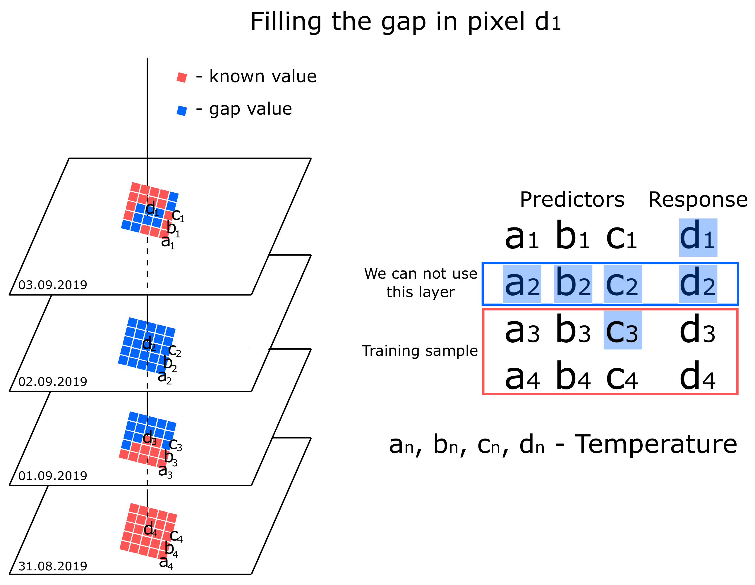
The proposed gap-filling approach is based on the following idea: for each gap pixel, a separate model is built. This model restores the gap based on the known values in pixels in the same image. Thus, the predictors are the known values selected in pixels of this image in a certain way.

We can approximate the connections between pixels based on historical data. An approximating function can be a machine learning algorithm. For most of these algorithms (linear regression, random forest, support vector method, k-nearest neighbors), it will be enough to use several hundred images for training the model. The conceptual scheme for selecting predictors is shown in Figure 1.

As can be seen from the figure, the previous images for this territory are used as a training sample. Predictions are based on machine learning methods, for now, LASSO regression, k-nearest neighbors, random forest, and the support vector regression are implemented. We can describe the model using the Equation (1):

$$D_{ijt}=F(T_{11k},T_{21k},T_{12k},T_{22k},\dots ,T_{nmk})$$

(1)

where $D_{ijt}$ is the temperature value in a closed cloud pixel with the indexes i row, j column, t is the time when the image was taken. $T_{ijt}$ is the temperature in known matrix cells with indices i row, j column, $t=k$ means that information from the same image is used to evaluate the value in the gap, without using predictors from previous $(k-1)$ images or subsequent $(k+1)$ ones, and F is a function that can be approximated by various machine learning algorithms, such as linear regression or random forest.

The most important step for such an approach is to select pixels-predictors. Predictors can be selected based on three strategies. The first strategy is to use all known pixel values in the image as predictors. This approach requires a lot of computational resources, so the algorithm performance is very ineffective. On the other hand, potentially, in this case, we involve more information in the model. The second strategy is to use 100 randomly selected points on the image. In this case, the algorithm works quickly, but the result is not accurate enough. The third strategy is to use as predictors only values from pixels that belong to the same biome (or land cover class, or another categorical feature) as the gap. If there are too many known pixels from the same biome, the 40 nearest points (according to the Euclidean metric) from this biome are used. For the sentinel-3 satellite system, it is possible to get a matrix of territory landscapes as an additional layer from a standard product (Figure 2). A similar dataset is also available for MODIS with MCD12 product.

By using a land cover matrix, pixels can be divided into groups that have different behaviors in terms of heat absorption and radiation. An example of the difference between the temperature distribution across biomes compared to the overall distribution in the image can be seen in Figure 2.

It shows that the temperature distribution across biomes is different. Thus, the approach based on the separation of the temperature field by biome allows us to achieve high accuracy along with a small runtime. The disadvantage of this strategy is the need to get a matrix (in this case, a biomes matrix) which divides pixels in images into groups. On the other hand, it allows us to use data about the internal structure of the territory, which significantly improves accuracy.

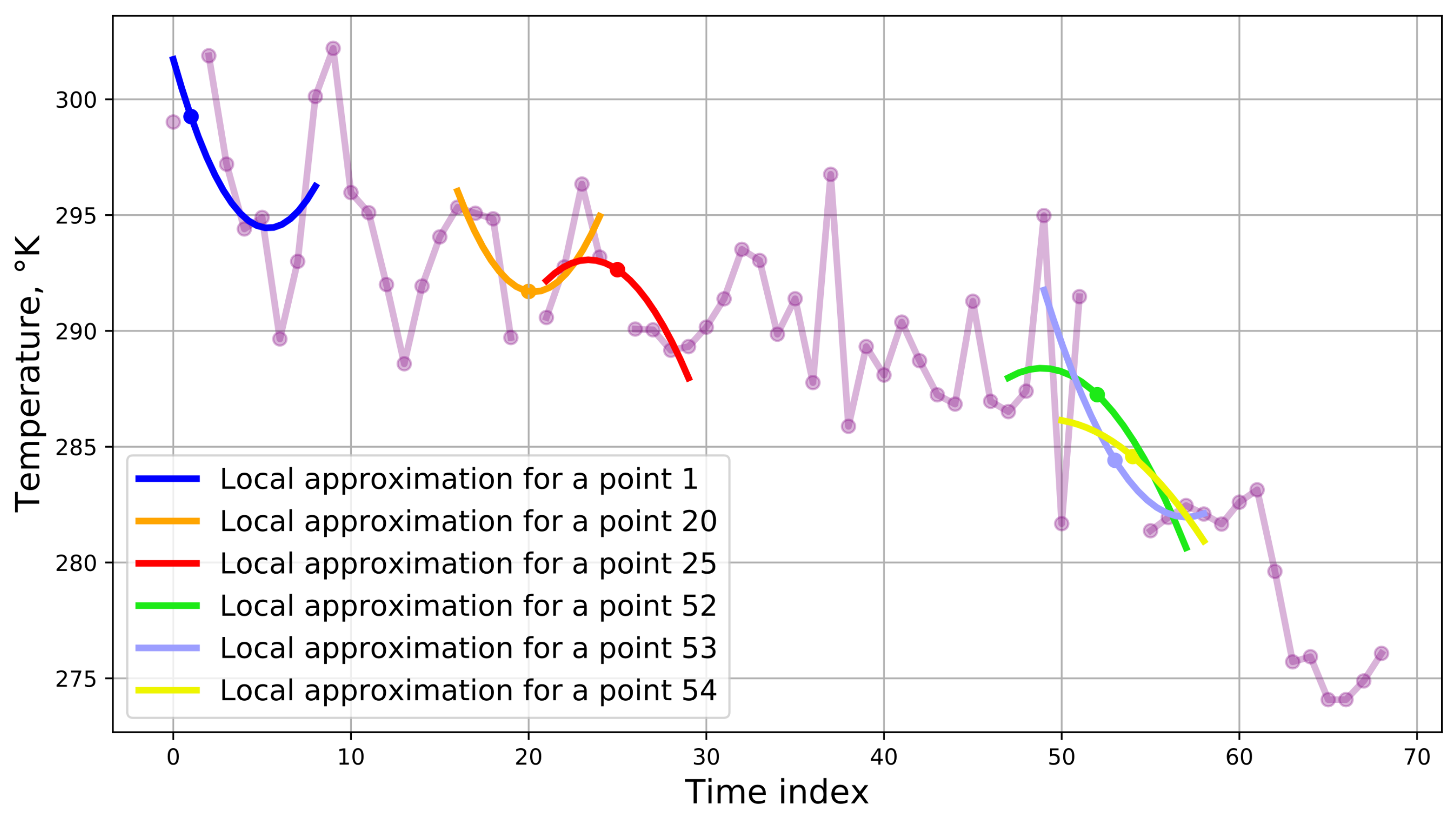
If the image was completely covered by the cloud, it is not possible to restore the values using the described approach. In this case, time series construction is used to fill in the gaps. In other words, images are placed on a regular time series grid. The sampling procedure can be performed with any time step size. The resulting gaps in the time series are restored using a locally median value or using a local approximation by a n degree polynomial constructed from k known neighboring points, where n is the given degree of the polynomial, and k is the number of points adjacent to the gap that the coefficients of the polynomial function are estimated from. In the example, n is equal to 2 and k is equal to 5 (Figure 3).

We can describe such a model as follows:

$$F\left(x\right)=a_0+a_{1}t+a_2{t}^2$$

(2)

where $a_0$, $a_1$, $a_2$ are coefficients of the polynomial function, t is time index. To estimate the coefficients of a polynomial function, the k known values closest to the gap are used. The described algorithm is shown in pseudocode (Algorithm 1).

Algorithm 1: Pseudocode of the algorithm for restoring gaps in time series using iterative approximation by polynomial functions

Data: array_with_gaps;  n = degree of a polynomial function;  k = the number of known elements for evaluating the coefficients of the polynomial;  Result: array without gaps  gaps ← all gap elements in array_with_gaps  for gap in gaps do  end

The presented approach was described in the article [55] and widely used. However, in the current implementation, we do not use a moving window for smoothing the series, but only for the task of restoring gaps.

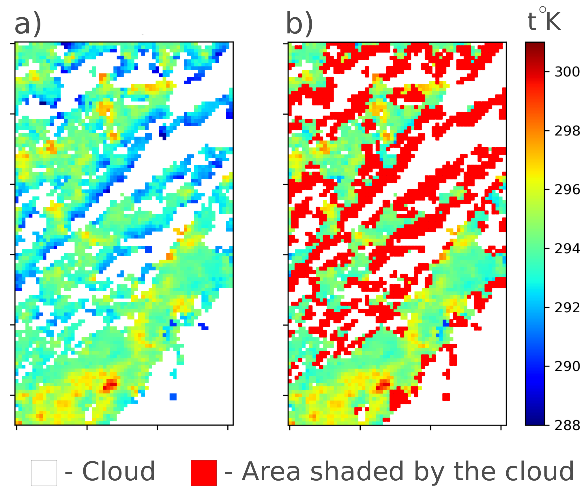
When experimenting with different cases, we also note an important feature of processing LST data. Some pixels of an image are not cloudy, but strongly affected by cloud cover, usually because they were cloudy shortly before the moment of sensing, or because of cloud shadows. Since the implemented gap-filling algorithm relies on known pixel values in the image, when using “shaded” pixels as predictors, the restored values in the gap will also be underestimated.

If the specific task of the gap filling is to get images that characterize the average temperature distribution in the absence of clouds, rather than at the specific time, then it is appropriate to use an approach to exclude pixels shaded by clouds. A cellular automaton [56] can be applied to detect such shaded pixels. This block of the algorithm is optional, and the user could decide to use it as an additional mechanism to filter data or not. A probabilistic approach is used to determine shaded pixels. The probability of assigning a pixel to a shaded one is proportional to the number of neighboring (Moore’s neighborhood [56]) pixels covered by the cloud. The probability of assigning a pixel to a shaded one is greater for those pixels whose temperature is lower than the median temperature value for pixels from the same biome or land cover type. The result of the algorithm is shown in Figure 4.

Excluding shaded pixels before the gap filling procedure starts allows us to obtain more plausible temperature fields.

Due to the fact that the algorithm was tested not only on the LST data, below we present the equations that were used to calculate the Normalized Difference Vegetation Index (NDVI) and broadband albedo data. The following formula was used to prepare the NDVI data:

$$NDVI=\frac{p_2-p_1}{p_2+p_1}$$

(3)

where $p_1$ is reflectivity in MODIS channel 1 corresponding to the wavelength range from 0.620 to 0.670 $\times {10}^{-6}$ m and $p_2$ is reflectivity in MODIS channel 2, corresponding to the wavelength range from 0.841 to 0.876$\times {10}^{-6}$ m.

The following equation was used to prepare the broadband albedo data [57]:

$$a=0.16\times p_1+0.291\times p_2+0.243\times p_3+0.116\times p_4+0.112\times p_5+0.081\times p_7-0.0015$$

(4)

where $p_3$, $p_4$, $p_5$, $p_7$ reflectivity in MODIS channels 3, 4, 5 and 7. The ratio of recorded wavelengths and channels is appropriate:

• $p_3$ from 0.459 to 0.479 $\times {10}^{-6}$ m;
• $p_4$ from 0.545 to 0.565 $\times {10}^{-6}$ m;
• $p_5$ from 1.230 to 1.250 $\times {10}^{-6}$ m;
• $p_7$ from 2.105 to 2.155 $\times {10}^{-6}$ m.

The presented algorithms, as well as auxiliary scripts for data preparation, are available in the module repository.

2.2. Experimental Studies

To verify the model, images of territories located South of the city of Saint Petersburg (Russia), South of the city of Madrid (Spain), and the area near Vladivostok (Russia) were selected. Spatial coverage of such images is 1 degree of latitude per 1 degree of longitude for each area:

• “Saint Petersburg”: 30–31°E, 58–59°N;
• “Madrid”: 5–4°W, 39–40°N;
• “Vladivostok”: 132–133°E, 44–45°N;

Images of three different products were prepared for each territory: Sentinel-3 LST (single flights data with 1 km/pixel spatial resolution and daily temporal resolution), MOD11A1 (daily land surface temperature gridded composites with 1 km/pixel spatial resolution), and MOD11_L2 (single flights land surface temperature data with 1 km/pixel spatial resolution and daily temporal resolution).

A training sample was prepared for each product, which consisted of 250–350 images of the territory for the period from May to August 2019. To verify the model, September images were used, where 6 images were selected that did not have clouds. Each image generated gaps of various shapes and sizes, and then applied the implemented gap-filling algorithm. So, 8 different types of gaps were generated and take from 4 to 96% of the territory in the image.

The size and shape of the gaps were “copied” from historical data for this territory. Since the algorithm uses information about landscape types, a matrix of landscape types was prepared for each test area, which was obtained from the Sentinel-3 LST archives. To check the accuracy of the gap filling, 4 metrics were used: bias, mean absolute error, root mean squared error (RMSE) and more robust to outliers such as median absolute error (MedAE).

Bias can be calculated as follows:

$$Bias=\frac{{\sum }_{i=1}^n{y}_i-x_i}{n}$$

(5)

where n = number of elements in the sample, $y_i$ is the prediction and $x_i$ the true value.

Mean absolute error is calculated using the following formula:

$$MAE=\frac{{\sum }_{i=1}^n|y_i-x_i|}{n}$$

(6)

Root mean squared error can be calculated as follows:

$$RMSE=\sqrt{\frac{{\sum }_{i=1}^n{(y_i-x_i)}^2}{n}}$$

(7)

Median absolute error can be calculated as follows::

$$MedAE=median\left(\right|y_1-x_1|,|y_2-x_2|,...,|y_n-x_n\left|\right)$$

(8)

To prove the ability of the implemented algorithm to fill in gaps not only in the LST data, additional experiments were performed on NDVI and albedo data. For the mentioned (Saint Petersburg, Madrid, Vladivostok) test territories, datasets were prepared from the MODIS sensor (MOD09GA product (https://lpdaac.usgs.gov/products/mod09gav006/) daily gridded surface spectral reflectance composites with spatial resolution from 500 m/pixel to 1 km/pixel), where 50–52% gaps were generated.

3. Results

3.1. Validation of the Algorithm on LST Data

Searching for optimal combination, we tested (over same datasets) lasso regression, random forest, extra trees, support vector regression and k-nearest neighbours regressions with and without additional biomes matrix, applying grid search for hyperparameters fitting. In case with LST support vector regression with predictors from the same biome proved to be the most accurate for land surface temperature gap-filling. For example, for Madrid case with Sentinel-3 LST data, the average MAE value for the support vector regression was 0.95 °C, while the random forest model showed an average MAE of 1.06 °C. On the other hand, in cases with NDVI and albedo, random forest regression with predictors from the same biome outperforms other approaches. These configurations are used for further testing.

The results of restoring the source matrix after applying the Support vector regression are shown in Figure 5.

As can be seen from Figure 5, the approach proposed in this article provides good quality. The mean absolute error on this matrix was 0.4 °C. It is worth noting that such a good data recovery is not always possible. In this case, the temperature distribution in the image was typical for the territory, so the algorithm was able to estimate the missing values very well.

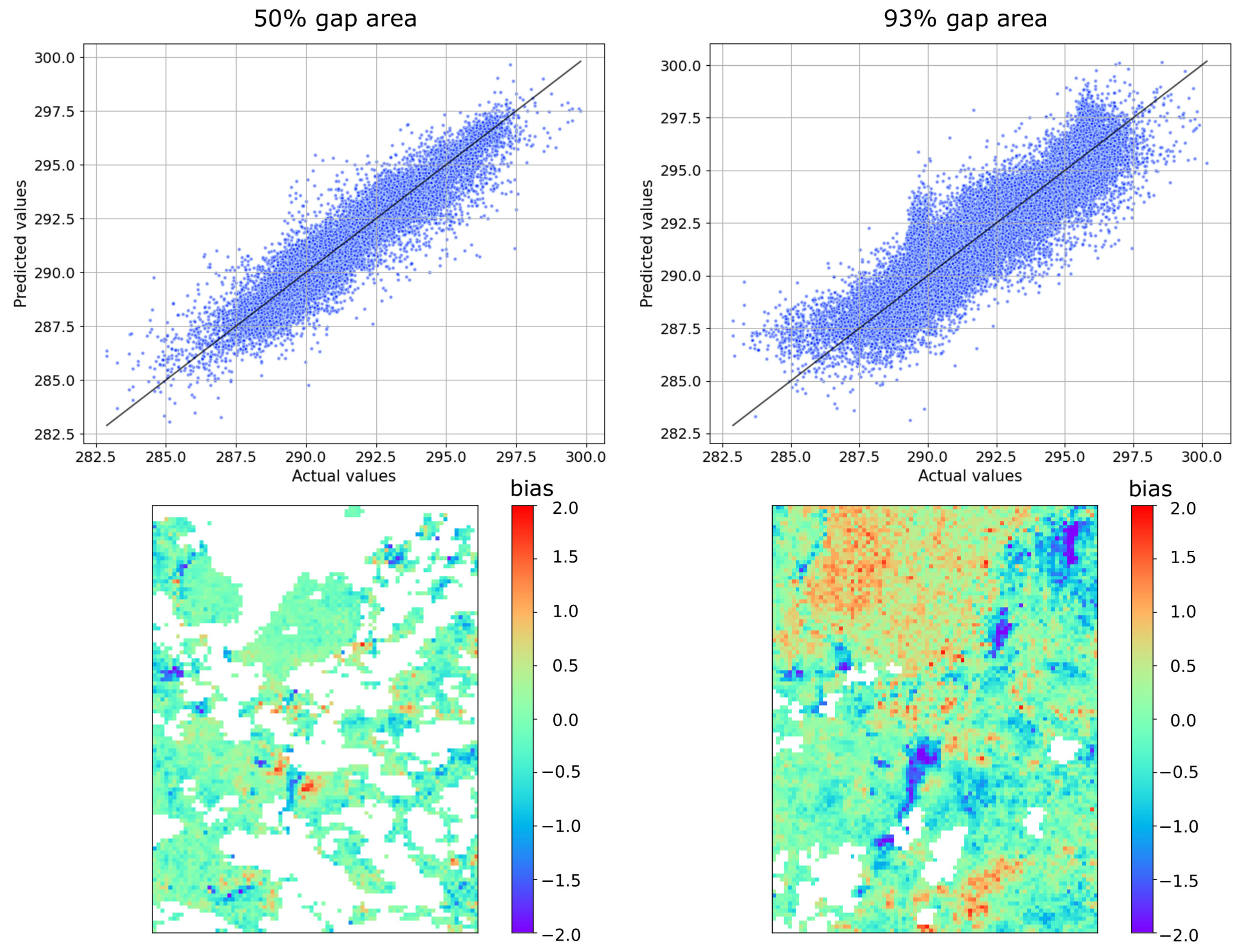
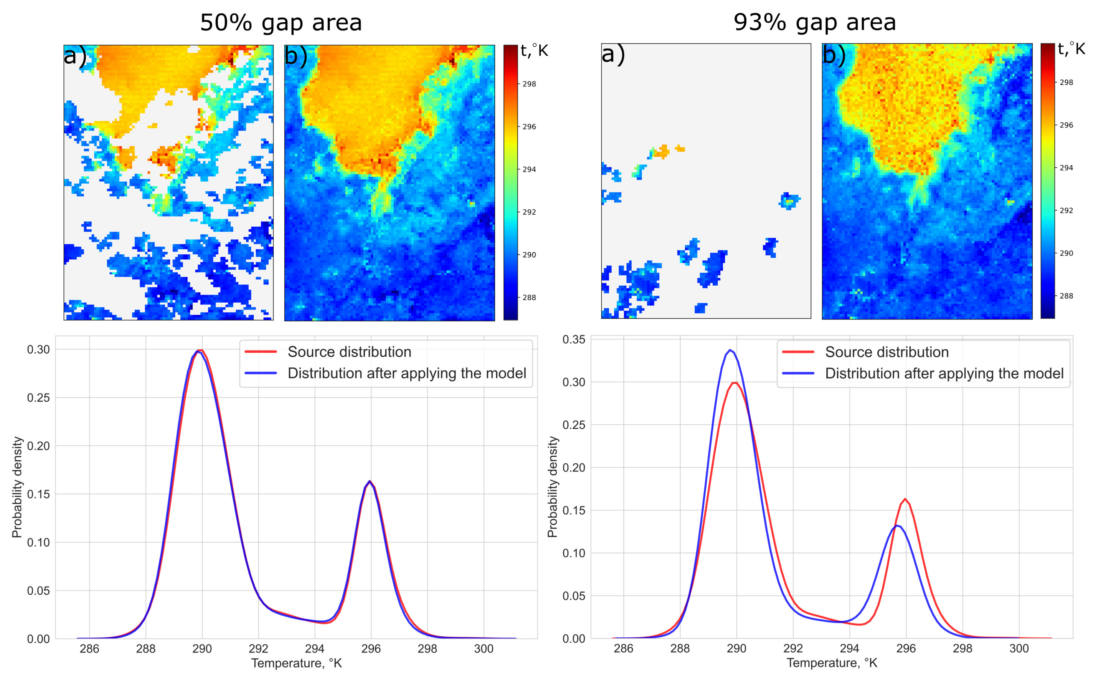
We can analyze the additional details of the gap filling results on Sentinel-3 LST data on the example of Vladivostok case. If we plot the temperature distribution for the above image before and after applying the algorithm, we get the following result (Figure 6).

As can be seen from the figure, for 50% gap size, the algorithm practically did not distort the original temperature distribution in the image. In the case of a 93% gap as expected, the recovery was worse. For Vladivostok case the average bias value for a 50% gap size was −0.084. For a 90% gap it was equal to 0.052.

The biplots for Vladivostok for all layers and the bias distribution in the gap can be seen in the Figure 7. To build such graphs, a certain type of gap (93% or 50%) was generated on 5 images, after which the omission was filled in by the algorithm. The values were averaged.

As can be seen from the Figure 7, in this case, the algorithm slightly overestimated the values for water objects. On the other hand, it can be seen that the algorithm on a large number of pixels gave unbiased forecasts.

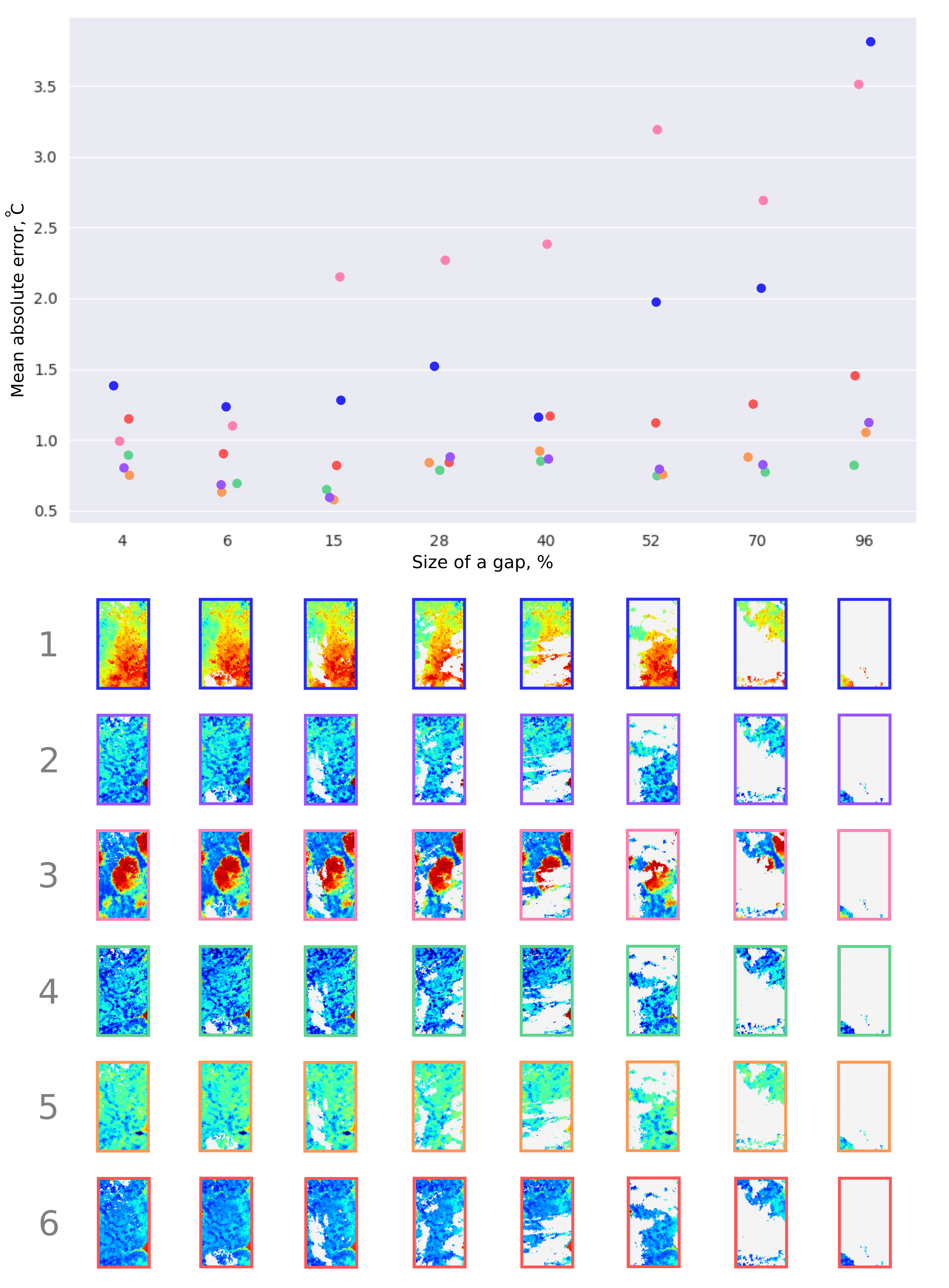
For the territory of Saint Petersburg for Sentinel-3 LST product, the value of Mean absolute error can be seen in Figure 8. The validation matrices are shown below the scatter plot, and the gaps that were generated for each case are shown in white.

Big values of MAE were obtained in fields 1 and 3, where we can notice patterns that are not typical for this territory. In other cases, the size of the gap did not significantly affect the accuracy of data recovery. So, for matrix number 3, the error of the algorithm on the 4% gap size was greater than for the 96% gap.

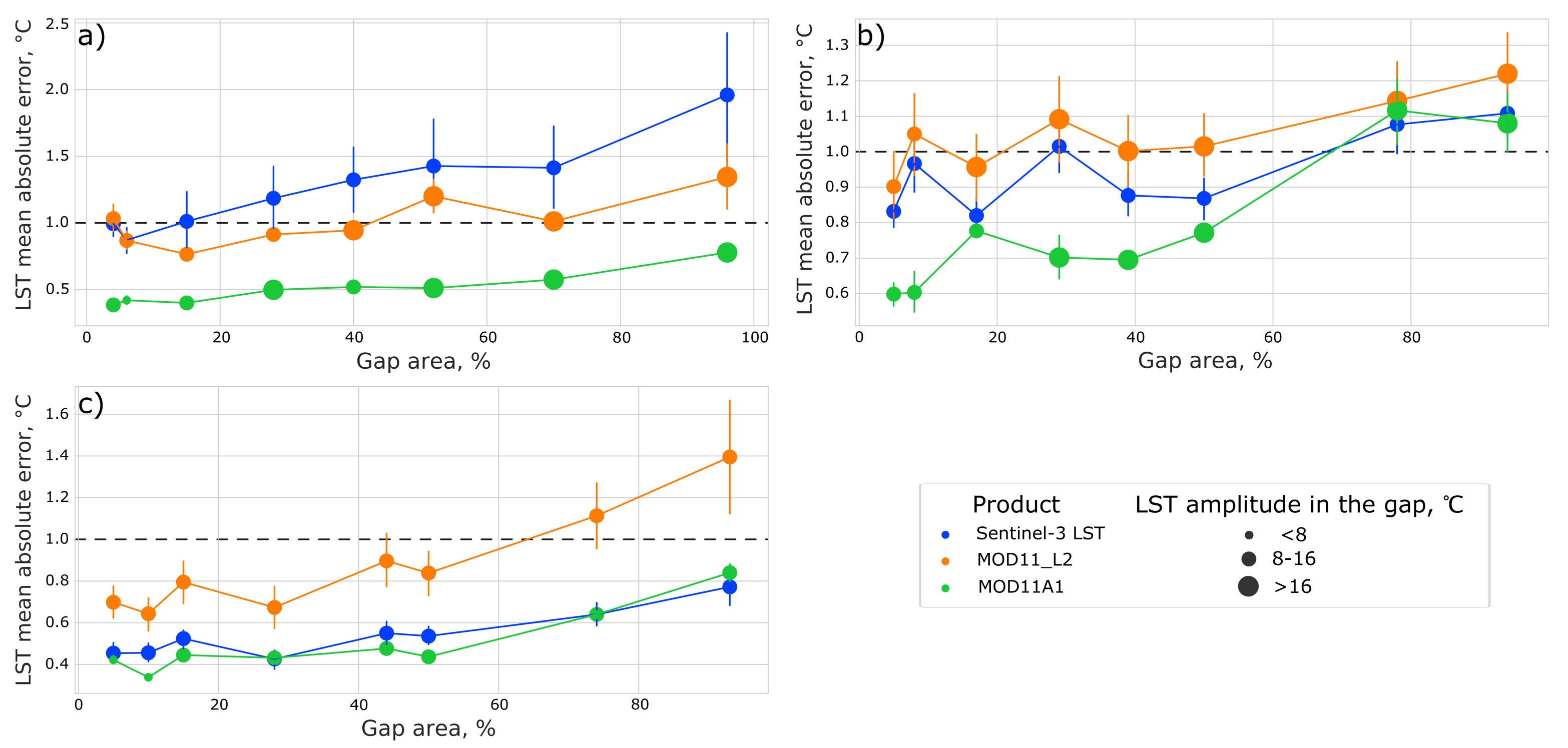
For each gap, we also calculated the value of the amplitude in it (the maximum value of the temperature in the gap minus the minimum value of the temperature in the gap). The results of the verification of the algorithm for various territories, products, and gap sizes can be seen in Figure 9.

As can be seen from Figure 9, the error of the algorithm increases as the size of the gap increases. However, this may not happen in specific matrices, it depends on the temperature distribution in the image. The temperature amplitude in the gap has little effect on the value of the mean absolute error.

Thus, the best results algorithm shows for the territory of Vladivostok since, in the images for this case, about 30% of the territory was occupied by a water object. Because of this, the temperature in the image changed very little in some areas.

Table 1. Algorithm validation errors.

Territory	Sentinel-3 LST			MOD11A1			MOD11_L2
	MAE	RMSE	MedAE	MAE	RMSE	MedAE	MAE	RMSE	MedAE
Saint Petersburg	11%	16%	8%	4%	5%	3%	6%	9%	5%
Madrid	8%	10%	7%	5%	6%	4%	6%	8%	5%
Vladivostok	5%	7%	4%	5%	7%	4%	8%	11%	6%

provides general information about the accuracy of the algorithm in various cases, namely MAE, RMSE and MedAE calculated as a percentage using the formula:

$$M_{perc}=\frac{M}{A}\times 100,\%$$

(9)

where M is the average MAE or RMSE or MedAE value for 6 images and 8 cloud types, A is the average temperature amplitude in the gap.

The table shows that in the vast majority of cases, the algorithm was able to reconstruct data with less than 10% MAE. The highest error values were obtained on Sentinel-3 LST data for the territory of Saint Petersburg, and the lowest was MOD11A1 for Madrid.

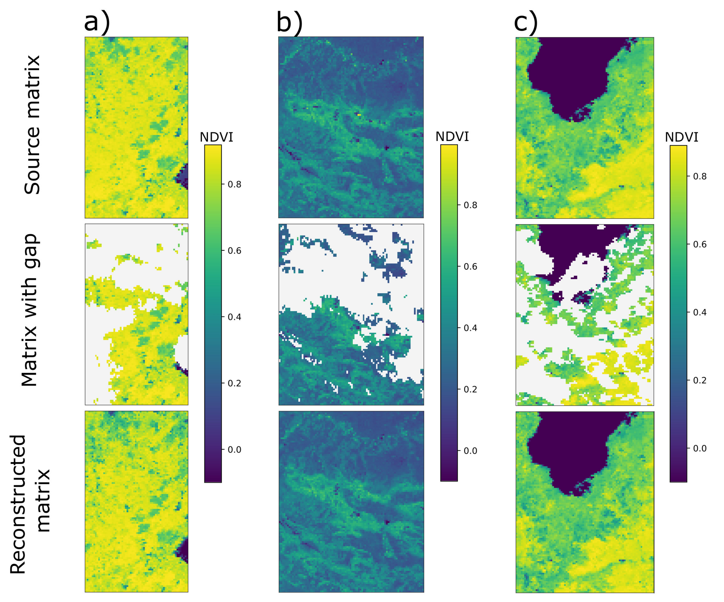
3.2. Validation of the Algorithm on NDVI and Albedo Data

The implemented algorithm can be applied not only to LST data, but also to other remote sensing products. As an example, the NDVI and albedo datasets are used.

We have prepared data based on the MOD09GA product from the MODIS sensor. To validate the algorithm, we used 6 images for 3 test territories:

• “Saint Petersburg”: 1 NDVI image and 1 albedo image for 5th of June 2019;
• “Madrid”: 1 NDVI image and 1 albedo image for 3rd of September 2019;
• “Vladivostok”: 1 NDVI image and 1 albedo image for 15th of September 2019.

On each such image, a gap with the 50–52% size was generated and then restored using a proposed algorithm.

For the algorithm to work correctly, a training sample was also prepared. For Vladivostok, 21 layers were prepared (data from September 12 to 18 for 2017–2019 years), for the territory of Madrid the value was 28 (data from August 31 to September 6 for 2017–2020 years), for the territory of Saint Petersburg the value was 28 (data from June 2 to 8 for 2017–2020 years). The results of filling in the gaps with Random forest regression in the NDVI data for 3 test territories can be seen in Figure 10.

As can be seen from the figure, the algorithm successfully coped with the task of restoring gaps in NDVI data. Some metrics for NDVI and albedo data restoration are listed in the

Table 2. Accuracy metrics for NDVI and albedo data. Column “Amplitude” NDVI or albedo amplitude in the gap, which can be calculated as “max value in the gap–min value in the gap”.

Case (NDVI)	Gap Area, %	MAE	RMSE	MedAE	Amplitude
Saint Petersburg	52	0.053	0.085	0.030	1.212
Madrid	50	0.028	0.053	0.016	1.128
Vladivostok	50	0.037	0.059	0.025	1.491
Case (Albedo)	Gap Area, %	MAE	RMSE	MedAE	Amplitude
Saint Petersburg	52	0.018	0.032	0.011	0.328
Madrid	50	0.013	0.025	0.009	0.536
Vladivostok	50	0.011	0.017	0.007	0.228

.

Thus, the algorithm successfully copes with the gap-filling on NDVI and albedo data with an average MAE value of about 5%, mean RMSE of 6% and mean MedAE of 2%.

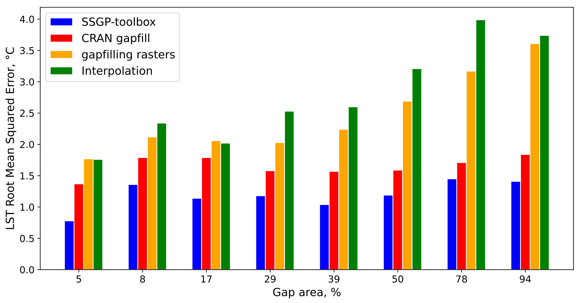
3.3. Comparison with “CRAN Gapfill” and “Gapfilling Rasters”

We compared our implemented algorithm with open-source competitors such as “CRAN gapfill” algorithm (https://cran.r-project.org/web/packages/gapfill/index.html) and “gap-filling rasters” (https://github.com/HughSt/gapfilling_rasters). We did not make a comparison with TIMESAT and gapfill-MAP, because these algorithms can not restore all the values in the gap. Moreover, authors of the article [20] compared these algorithms with the “CRAN gapfill”, which surpassed them in accuracy. Thus, in our comparison, we considered “CRAN gapfill” as the main competitor. A link to the dataset on which the comparison was made, with a detailed description of it, is provided in the Supplementary Materials).

To compare the algorithms, we selected three test territories near the cities of Saint Petersburg, Madrid and Vladivostok. Since the “CRAN gapfill” and “gapfilling rasters” algorithms require layers to be placed on a regular time series grid, the MOD11A1 product was used. For Vladivostok, 21 layers were prepared (data from September 12 to 18 for 2017, 2018, 2019), for the territory of Madrid, 28 (data from August 31 to September 6 for 2017, 2018, 2019, 2020), for the territory of Saint Petersburg, 28 (data from June 2 to 8 for 2017, 2018, 2019, 2020). Validation was performed on the image for 15 September 2019 for Vladivostok, for 3 September 2019 for Madrid and for 5 June 2019 for Saint Petersburg. Each image generated 8 types of gaps ranging in size from 4 to 96%. For SSGP-toolbox algorithm, we have used an additional layer, the biome matrix. A digital elevation model was prepared for the “gapfilling rasters” algorithm.

The results of comparing the accuracy of the SSGP-toolbox algorithm and its competitors “CRAN gapfill” and “gapfilling rasters” in the gap recovery task can be seen in the

Table 3. Comparison of gapfilling algorithms on LST data by Mean Absolute Error, °C.

Algorithm	Gap Size (Saint Petersburg Case)
	4%	6%	15%	28%	40%	52%	70%	96%	Mean
SSGP-toolbox	0.42	0.42	0.35	0.39	0.43	0.48	0.47	0.87	0.48
CRAN gapfill	0.8	1.28	0.94	0.99	1.31	0.98	1.08	1.07	1.06
gapfilling rasters	0.61	0.73	0.96	0.88	0.86	0.54	0.82	0.80	0.78
Nearest neighbour interpolation	0.59	0.68	0.55	1.10	1.12	1.02	1.00	1.22	0.91
Algorithm	Gap Size (Madrid Case)
	5%	8%	17%	29%	39%	50%	78%	94%	Mean
SSGP-toolbox	0.53	0.89	0.76	0.79	0.69	0.84	1.04	0.97	0.81
CRAN gapfill	1.03	1.19	1.39	1.17	1.11	1.19	1.32	1.42	1.23
gapfilling rasters	1.37	1.70	1.56	1.57	1.76	2.15	2.66	2.94	1.96
Nearest neighbour interpolation	1.26	1.74	1.41	1.91	1.75	2.20	2.90	2.77	1.99
Algorithm	Gap Size (Vladivostok Case)
	5%	10%	15%	28%	44%	50%	74%	93%	Mean
SSGP-toolbox	0.30	0.31	0.36	0.32	0.47	0.36	0.50	0.68	0.41
CRAN gapfill	0.47	0.36	0.58	0.43	0.59	0.55	0.84	0.73	0.57
gapfilling rasters	0.67	0.63	0.66	0.72	0.77	0.81	0.85	1.24	0.79
Nearest neighbour interpolation	0.40	0.43	0.44	0.47	0.53	0.56	0.90	1.01	0.59

. Nearest neighbour interpolation can be considered as a baseline.

As can be seen from the table, the SSGP-toolbox was more accurate than its competitors. Nearest neighbor interpolation and “gapfilling rasters” proved to be the least accurate algorithms.

The average error values for the Vladivostok case were lower since most of the image was taken up by a lake where the temperature amplitude was lower than on the land surface. The value of the errors was greater for the Madrid case (Figure 11).

For the Madrid case, the average value for MAE for SSGP-toolbox was 0.81 °C (RMSE = 1.19), while for “CRAN gapfill” the average MAE value was 1.23 (RMSE = 1.66). “gapfilling rasters” and interpolation showed similar results of 1.96 (RMSE = 2.46) and 1.99 (RMSE = 2.77), respectively. The average value of the temperature range in the gap (max LST value–min LST value) was 22.3 °C. Thus, the MAE for SSGP-toolbox was 4%.

The advantage of our approach is that there is no need to place matrices on a regular grid in time. On the other hand, the “CRAN gapfill” algorithm performs all operations in less time and can also be effectively parallelized.

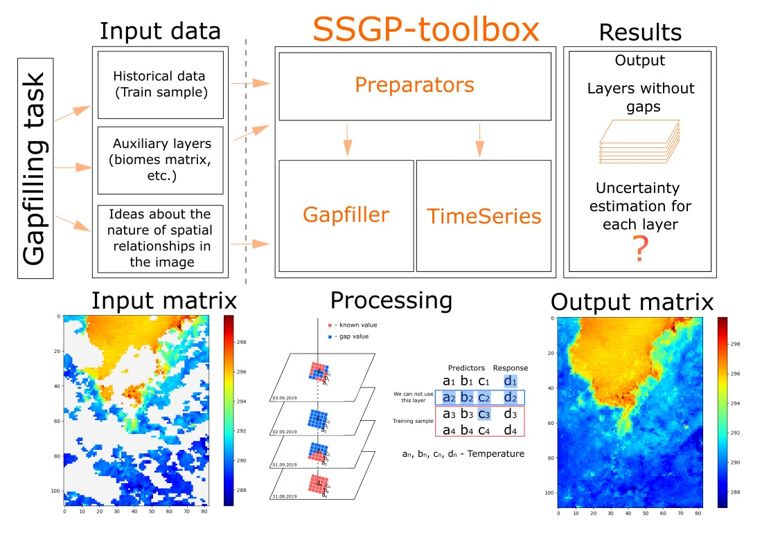
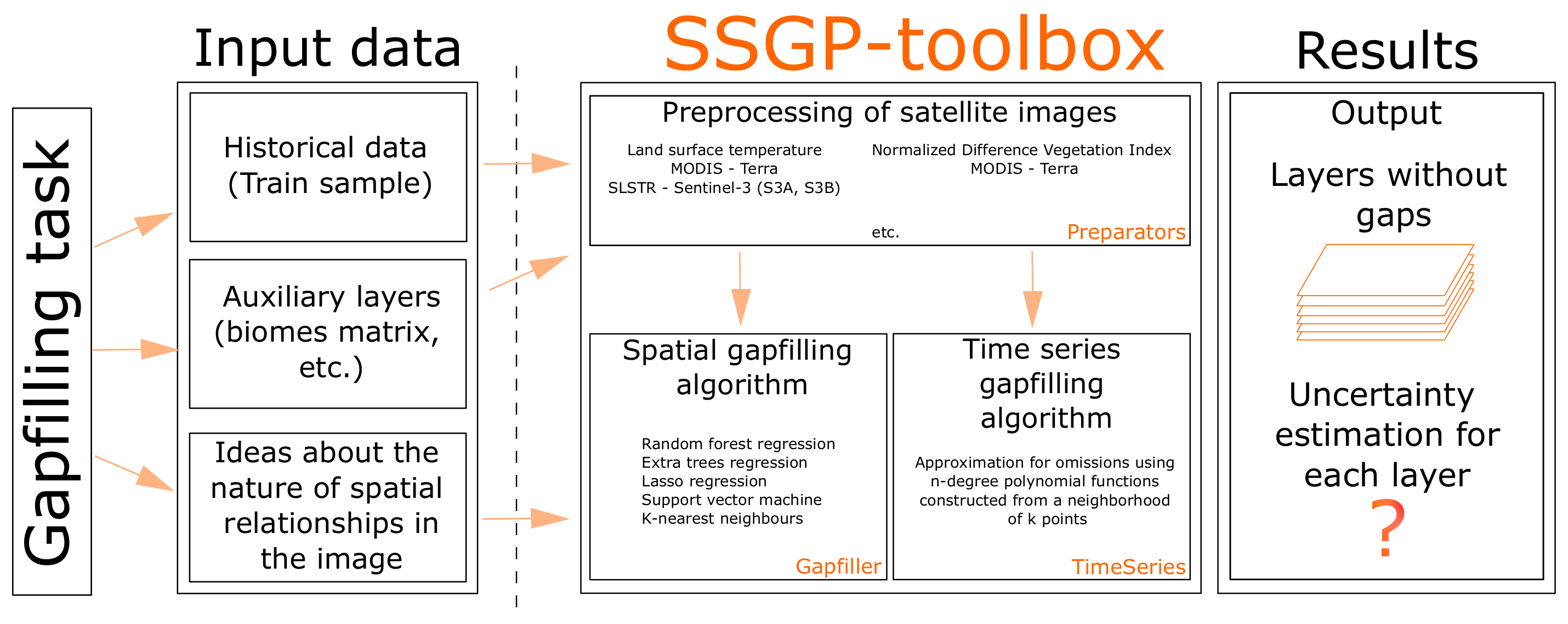
3.4. Software Implementation

The software implementation of the algorithm is developed in Python (popular in the field of environmental studies) and called SSGP-toolbox (Simple Spatial Gapfilling Processor-toolbox). A link to the module repository is available in Supplementary Materials.

The diagram of the implemented module can be seen in the Figure 12.

Thus, we have divided the algorithm into several blocks that can be used independently of each other.

To launch gap-filling process we need to prepare matrices in binary format and place them in a certain way in the file system. The placement of matrices in directories and subdirectories should be done as follows. It is needed to prepare three folders if we want to use the land type matrix: “Extra”, “History” and “Inputs”. If we do not plan to use the extra matrix, there will be a need to create the “History” and “Inputs” folders. The “History” folder contains matrices on which the algorithm will be trained. However, there is no need for matrices in the training sample to be without gaps. The “Inputs” folder contains the layers that need to be filled in. The “Extra” folder contains the “Extra” matrix. The “Extra” matrix can be, for example, a matrix of landscape types or any other means in current case values. As a result of the algorithm, the “Outputs” folder is formed, where layers without gaps are located. Various visualizations and a more detailed explanation of the working directory structure are provided in the module repository.

If there is a need to build time series, we can use the TimeSeries module, which can place layers on the time series and fill in gaps using local approximations with polynomials functions. The result of the algorithm is gap-filled binary matrices. It is optionally possible to generate netCDF as an output format. SSGP-toolbox also provides several functions to automatically prepare SLSTR and MODIS products to use with the toolbox.

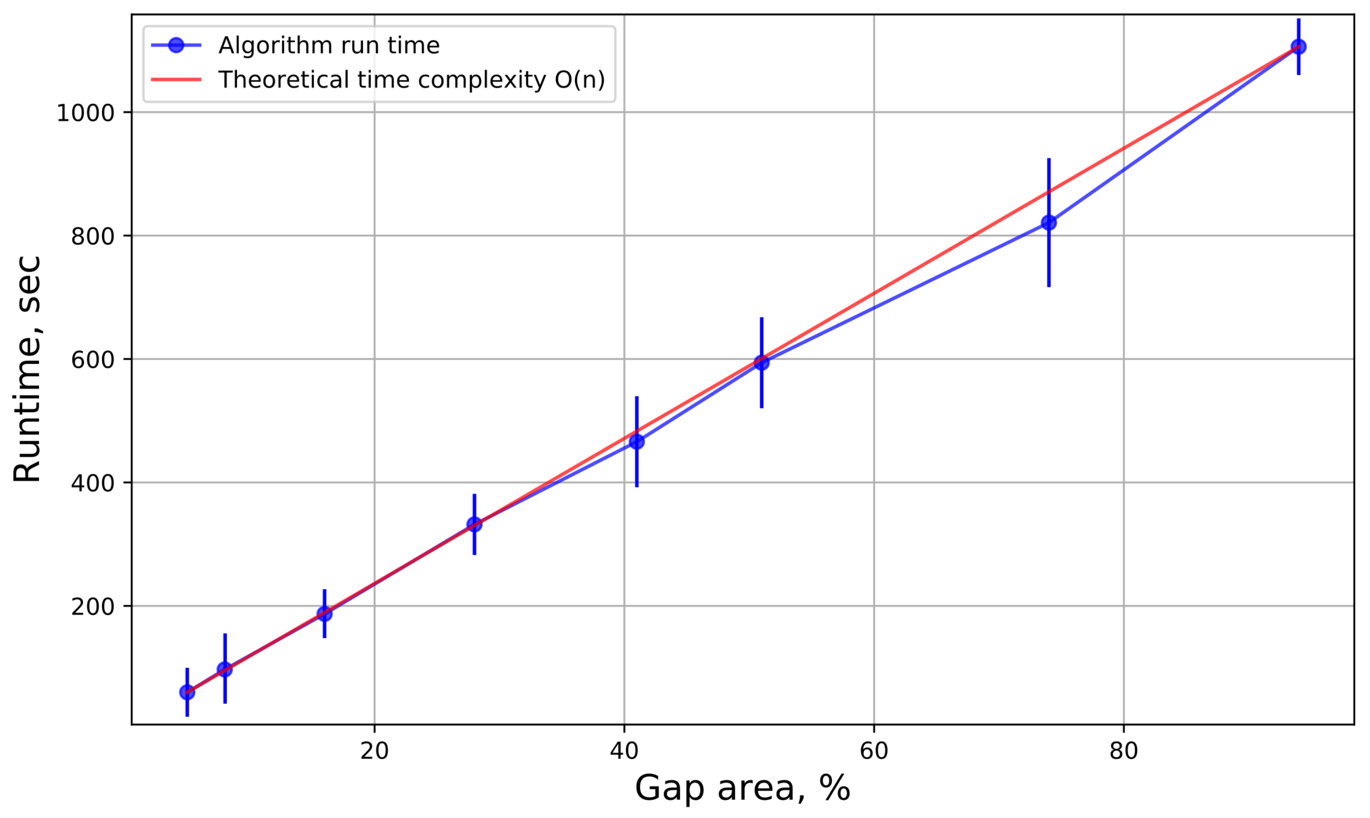
The time complexity estimation (Figure 13) was performed for the gap filling algorithm. The running time of the algorithm was recorded for each territory and each product, and the time was averaged.

As can be seen from the graph, the time complexity of the algorithm is linear. This is confirmed by the method of constructing models, for each pixel with a gap, its own model is built, therefore, with an increase in the number of missing pixels, the processing time will also increase proportionally. On the other hand, the training time of models is greatly affected by the size of the training sample. Therefore, if there is a need to speed up the algorithm, we can reduce the size of the training sample by removing some layers from the “History” folder.

4. Discussion

4.1. Accuracy of Data Recovery

Thus, we verified the algorithm on 424 Land Surface Temperature matrices (3 remote sensing products × 3 test territories × 6 images for particular area × 8 types of gaps minus 8 because of the Vladivostok case, 5 images were used for Sentinel-3 product instead of 6), 3 NDVI and 3 albedo matrices. The accuracy was also compared with the similar open-source packages: “CRAN gapfill” and “gapfilling rasters”.

To model the relationships between pixels for LST data, we used the linear model, the support vector machine. Good accuracy of data recovery means that it is sufficient to use linear models to restore values in temperature fields. However, if the dependencies are nonlinear, for example, it is possible for other remote sensing products, then a random forest or the support vector method on a polynomial kernel can be used as the core of the SSGP-toolbox. For example, a random forest was used to effectively restore the NDVI and albedo fields.

In the vast majority of cases, the MAE value did not exceed 1 °C for LST data. After conducting experiments to test the algorithm on gaps of various shapes and sizes, it was found that the accuracy of data recovery decreases slightly when the gap size in the image increases. At the same time, the algorithm can restore the values fairly accurately if the temperature field is typical for the considering territory. If there were not enough similar matrices in the training sample, this may lead to an increase in the error. If the image is completely covered by clouds or the known values in the image are not enough to build spatial models, then the algorithm to restore missing values in time series can be applied. The use of local approximation by polynomial functions allows us to estimate the values in the gaps. However, the accuracy of this algorithm is lower than that of the “spatial gapfiller”: as a result of experiments, it was found that for Land Surface temperature data, the average value of MAE when using the “spatial algorithm” was less than 1 °C, and for the algorithm of local approximation by polynomials it was 3 °C.

For NDVI data, the MAE did not exceed 0.06 conventional units. For albedo data, the MAE was less than 0.02 in all cases. Thus, the $MA{E}_{perc}$ was less than 5%. The accuracy of the gap-filling algorithm on this data is higher than on LST data. This is because NDVI and albedo are more stable parameters during the days.

4.2. Applications for Different Remote Sensing Products

We built the software implementation in such a way that the core of the algorithm remains unchanged when used for various remote sensing products. So, the matrices for using the module can be prepared using the “Preparators” block, which currently includes submodules that allow preparing land surface temperature data from the Sentinel-3 satellite system from the SLSTR sensor (Sentinel-3 LST), land surface temperature data from Terra satellite from MODIS sensor for MOD11A1 and MOD11_L2 products, as well as for MODIS reflectance products (MOD09GA).

If necessary, custom algorithms and software to process certain remote sensing products can be applied. The main thing is that after preprocessing the matrices are given in npy format and were located in the directory as specified in the documentation.

4.3. Limitations

The core of the SSGP-toolbox module is divided into two blocks. The first one, “Gapfiller”, allows us to build models for restoring gaps based on known pixels in the image. For this module to fill in the gaps, there is a need for more than 100 known pixels in the image, and the overall size of the matrix is not important. Within this block, it is not possible to fill in gaps with the number of predictors less than 100. But in this situation, the second block—“TimeSeries”—can help. The “TimeSeries” submodule can discretize a time series with a given time step, if necessary. It also has methods for restoring gaps in time series, that allows us to evaluate values in omissions even if the image was completely obscured by the cloud. But the accuracy of this recovery is lower than using spatial relationships.

Thus, the presented algorithm has no restrictions on the size of the gap. However, the efficiency of the algorithm is affected by the size of the matrices and the training sample. This is because the module builds pixel-by-pixel approximations, so the more models we need to train, the longer the algorithm will run. In other words, on matrices with a size of 100 by 100 elements and a training sample size of 300 images, it will not be hard to fill in large gaps with a size of 9900 pixels in a few tens of minutes. On the other hand, if we need to restore values on matrices with a size of 10,000 by 10,000 elements, then this algorithm will work for a very long time on a laptop. The solution to this problem may be to run the algorithm remotely on the server or to reduce the training sample. The size of the training sample may depend on the specific conditions of the task. But if the images without gaps are available to train the algorithm, then 3 matrices are enough to achieve the appropriate quality.

5. Conclusions

An approach to fill gaps in land surface temperature, NDVI and surface albedo remote sensing data using machine learning techniques was presented and validated. The proposed method integrates support vector machines algorithm (for LST data), random forest regression (for NDVI and albedo data) and special techniques for selecting training scenes and anchor pixels, implying that connections between pixels are stable enough to restore values in gaps. The spatial and temporal approaches were combined to make it possible to fill in gaps even when 100 percent of the image was covered by clouds. The developed model was implemented as a python-based toolbox and was published as an open-source module on GitHub.

The algorithm was verified on three remote sensing LST products (Sentinel-3 LST, MODIS MOD11A1, MODIS MOD11_L2). Validation experiment includes 3 territories (1x1 degree areas around Saint Petersburg, Madrid and Vladivostok), and 6 images with 8 generated cloud masks, covering from 4 to 96% of the image. So, the experiment covers 424 validation images under different climate and cloud cover conditions. The mean absolute error in most cases did not exceed 1 °C and 10% in relative value, which is enough for most environmental cases, both retrospective and operational tasks.

The verification was also performed on NDVI and albedo data (MOD09GA product). The relationships between cells in these matrices are non-linear, so the random forest regression was used to approximate the dependencies. The verification results on 3 test territories showed that the algorithm’s MAE for NDVI did not exceed 0.06, and for the albedo data it was in all cases less than 0.02.

Comparative testing with open-source competitors (such as “CRAN gapfill” and “gapfilling rasters”) has shown that our algorithm is able to more accurately restore surface temperature data in the gaps with fewer restrictions imposed on the data sources. SSGP-toolbox can be applied not only to data (images) observed at equally-spaced points in time.

The fact of successful land surface temperature, NDVI and albedo data reconstructions based on values of the same scene pixels is evidence of strong connections between values of neighboring areas and the existence of stable patterns.

By publishing open-source implementation, we hope to involve remote sensing scientists and engineers to test, use, and develop approaches to reconstructing missed values in time-series satellite data.