2.1. Fusion of Multi-Satellites Snow Depth Estimations
For GNSS receivers fixed on the ground with a zenith-looking antenna, the received GNSS signal is the interferometric signal, which consists of the direct GNSS signal and reflected GNSS signals. The strength of the received GNSS signals and noise level are recorded by the GNSS receiver as SNR observations. The direct component of the SNR observations can be modeled as a low-order polynomial in general and removed from SNR observations to obtain the multipath SNR observations (or detrended SNR observations), which can be written as [
11]:
where
A is the amplitude of multipath SNR signal;
H is GNSS antenna height when the ground is covered by snow;
λ is the GNSS signal wavelength of interest;
θ is the GNSS satellite elevation angle; and
f is the main frequency (or spectral peak frequency) of SNR observation series. Note that Equation (1) only considers the specular reflection path for simplicity in the theoretical analysis. In fact, because of the influence of the reflecting surface roughness and variety of snow layers on the GNSS signal, the realistic reflection of GNSS signals is diffused and the GNSS antenna would capture signals reflected from many points. However, among all the captured reflected signals, the signal reflected at the specular point has the shortest propagation path and the signal energy captured by the antenna mostly comes from the signals reflected around the specular point. This is the reason why one may only consider the specular reflection path for simplicity in theoretical analysis.
The series of multipath SNR observations is a quasi-sinusoidal signal periodically oscillating with respect to the sine of the elevation angle [
13]. If the sine of the elevation angle is taken as the independent variable, the main frequency of the series
f has a relationship with the antenna height (
H) relative to the snow-covered ground surface as:
If the antenna height in the snow-free case
H0 is known in advance, the snow depth
h can be estimated by:
Clearly, the precision of SNR-based snow depth estimations depends on the precision of the SNR series main frequency estimation, which is obtained by spectral analysis suited for unevenly sampled data such as Lomb-Scargle spectral analysis. The unmodeled multipath interference and receiver noise would contaminate the multipath SNR observation series, and produce the bias in the peak frequency of the series, degrading the snow depth estimation accuracy [
17]. The antenna height estimation obtained by Equation (2) is based on the assumption that there is only one layer of snow reflecting the GNSS signal. In reality, there may be several snow layers reflecting the signals. GNSS signals reflected from the inner layers would interfere with the signals reflected over the top layer, resulting in an overestimation of antenna height and thus underestimation of snow depth [
13]. Correction of the bias would improve the accuracy of the snow depth estimation; however, it is non-trivial to model and remove the bias. Nevertheless, it is useful to develop a technique to model and remove the bias in the future.
Figure 1 shows an example of simulated multipath SNR series of GPS L1 signals and the results of the Lomb-Scargle spectral analysis. The antenna height is set at 2.5 m, and the surface is flat; the radiation pattern of GNSS antenna TRM55971.00 and a typical complex dielectric constant of dry snow (2-0.0005j) are used for the calculation of the amplitudes of the SNR series [
14]. For convenience, three Gaussian noise components are respectively added to the noise-free SNR series to produce three noise-corrupted series with different noise levels. The three SNR values (denoted by S/N) of those three simulated multipath SNR series are 15 dB, 10 dB and 5 dB, respectively. It can be observed that the presence of noise results in variation in the peak frequencies; stronger noise causes a larger peak frequency shift. The peak frequency error is about 0.4 when the S/N of the simulated multipath SNR series is 5 dB. The peak frequency error would lead to a bias of about 4 cm in snow depth estimation for GPS L1 signals. Thus, a quantitative indicator of the noise level is useful, as the noise level indicates the precision of the peak frequency estimation, and hence, the snow depth estimation precision. It can also be seen from
Figure 1 that the peak of the power spectral density (PSD) is inversely proportional to the noise level. This implies that the peak of the PSD obtained by the spectral analysis on the multipath SNR series could be used as an indicator of the precision of the peak frequency estimation.
To evaluate the impact of noise, 20 different Gaussian noise levels are selected, corresponding to the S/N from 1 dB to 20 dB with an interval of 1 dB. For a given noise level, 1000 noise sequences are generated, and each of them is added to the noise-free multipath SNR series to produce a noise-corrupted multipath SNR series. Then, the Lomb-Scargle spectrum analysis is applied to the SNR series to obtain the peak PSD and the corresponding peak frequency. Subtracting the peak frequency from the theoretical one in the noise-free case produces the noise-induced frequency error. Repeating the procedure for all other 999 noise-corrupted multipath SNR series under the same noise level, a sequence of 1000 peak frequency errors and 1000 peak PSD values are obtained. After repeating the procedure for all other 19 noise levels, 20,000 samples are obtained for the peak frequency error, corresponding to 20,000 samples of peak PSD.
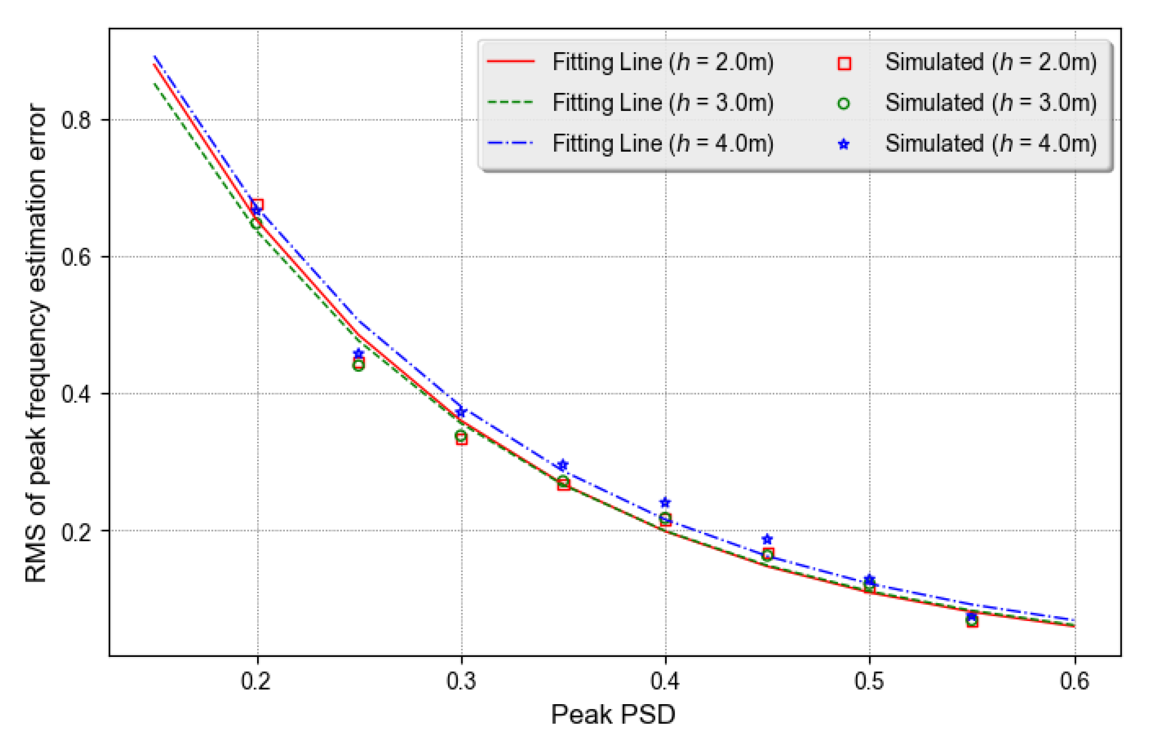
All the peak PSD samples are arranged into bins centered at eight different peak PSD values (0.2, 0.25, 0.3, 0.35, 0.4, 0.45, 0.5 and 0.55), and the width of each bin is 0.05. Each of the central peak PSD values represents all the peak PSD samples within the bin. The root mean square (RMS) of the peak frequency error within each bin is calculated. Thus, a distribution of the RMS of the peak frequency error versus the peak PSD is obtained, as shown in
Figure 2, where three different antenna heights are tested. Obviously, the RMS of the peak frequency error decreases with the increased peak PSD. The RMS of the peak frequency error is marginally different under different antenna heights. However, the variation pattern of the RMS of the peak frequency error versus the peak PSD is almost the same. Using the exponential fitting produces the exponential fitting functions as:
where
α and
β are the fitting parameters and
p is the peak PSD. The fitting curves under three different antenna heights are also shown in
Figure 2. The correlation coefficients between the simulated and the fitted RMS of peak frequency error are 0.9903, 0.9907 and 0.9877 for three different antenna heights, respectively, indicating a valid fitting. In addition to the three antenna heights (2.0 m, 3.0 m and 4.0 m), six more antenna heights (1.0 m, 1.5 m, 2.5 m, 3.5 m, 4.5 m and 5 m) are also tested, producing nine groups of two fitting parameters (
α and
β) and one group of correlation coefficients (
R), as shown in
Table 1. It can be seen that all of the correlation coefficients between the simulated and fitted RMS of the peak frequency error are larger than 0.98. The fitting parameter
α ranges from 1.9 to 2.2, while the fitting parameter
β varies between −6 and −5. As those two fitting parameters are not sensitive to the antenna height, it is reasonable to take the average of each parameter series as the final value. Then, the exponential fitting function of Equation (4) can be rewritten as:
Since the precision of SNR-based antenna height estimation and that of snow depth estimation are proportional to precision of spectral peak frequency estimation, the exponential function in Equation (5) can be used to weight snow depth estimations related to individual satellites. Thus, a fusion model is developed to combine multi-satellites snow depth estimations in a given period (e.g., a day) as:
where
hi is SNR-based snow depth estimation for the
i-th GNSS satellite. Substituting Equation (5) into Equation (6), the weighted average snow depth fusion model can be written as:
where
pi is the peak PSD of multipath SNR observation series for the
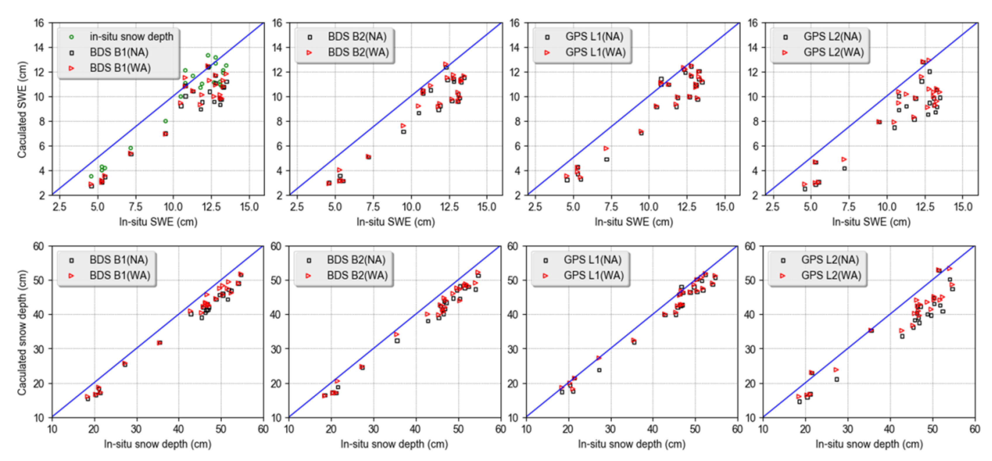
i-th GNSS satellite. Assume that the GNSS antenna height is 5.0 m when ground is snow-free and consider eight different snow depths ranging from 0.5 m to 4.0 m with an interval of 0.5 m. For each snow depth, five SNR series are produced with noise levels of 2 dB, 4 dB, 6 dB, 8 dB and 10 dB, respectively. Each noise-corrupted SNR series is used to generate a snow depth estimate. Then, the normal average method (NA) and weighted average (WA) method are used to determine the final snow depth estimate. Repeating the procedure 200 times, 200 normal average estimates and 200 weighted average estimates are produced for each antenna height. This simulation result shows that the RMS of the snow depth estimation error is 0.91 cm for the former and 1.37 cm for the latter. The relative snow depth estimation accuracy has improved considerably (about 34%) by using the weight average fusion model. Note that, although Equations (5) and (7) are obtained based on the simulation of GPS L1 band signals, simulation results, including GPS L2 and L5 and BDS B1, B2 and B3 band signals show that the difference of the fitting parameters in the weighted average snow depth fusion model is marginal for different GNSS band signals if the GNSS antenna gain pattern is not significantly different. In addition, the performance of the weighted average snow depth fusion model for BDS B1 and B2 and GPS L1 and L2 signals based on snow depth observations has also been evaluated in
Section 4.1.


