Article

How Does Peri-Urbanization Trigger Climate Change Vulnerabilities? An Investigation of the Dhaka Megacity in Bangladesh

School of Built Environment, Queensland University of Technology, 2 George Street, Brisbane, QLD 4000, Australia
*
Author to whom correspondence should be addressed.
Remote Sens. 2020, 12(23), 3938; https://doi.org/10.3390/rs12233938
Submission received: 24 October 2020 / Revised: 29 November 2020 / Accepted: 30 November 2020 / Published: 1 December 2020
(This article belongs to the Special Issue Remote Sensing of Natural Hazards)

Abstract

:
This paper aims to scrutinize in what way peri-urbanization triggers climate change vulnerabilities. By using spatial analysis techniques, the study undertakes the following tasks. First, the study demarcates Dhaka’s—the capital of Bangladesh—peri-urban growth pattern that took place over the last 24-year period (1992–2016). Afterwards, it determines the conformity of ongoing peri-urban practices with Dhaka’s stipulated planning documents. Then, it identifies Dhaka’s specific vulnerabilities to climate change impacts—i.e., flood, and groundwater table depletion. Lastly, it maps out the socioeconomic profile of the climate change victim groups from Dhaka. The findings of the study reveal that: (a) Dhaka lacks adequate development planning, monitoring, and control mechanisms that lead to an increased and uncontrolled peri-urbanization; (b) Dhaka’s explicitly undefined peri-urban growth boundary is the primary factor in misguiding the growth pockets—that are the most vulnerable locations to climate change impacts, and; (c) Dhaka’s most vulnerable group to the increasing climate change impacts are the climate migrants, who have been repeatedly exposed to the climate change-triggered natural hazards. These study findings generate insights into peri-urbanization-triggered climate change vulnerabilities that aid urban policymakers, managers, and planners in their development policy, planning, monitoring and control practices.

Graphical Abstract

1. Introduction

Due to the global urbanization drives, major metropolitan cities and regions across countries are gradually expanded by continuously encroaching their physical growth boundaries into adjoining peri-urban areas [1,2,3,4]. Hence, urban growth at present predominantly is occurring in the form of peri-urbanization globally [5]. Thus, rapid peri-urbanization has already become an issue of increasing global concern [6]. In addition, peri-urban areas are also vulnerable to climate change impacts [7,8]. Consequently, these peri-urban growth pockets provoke considerable growth challenges to policymakers [9,10,11].
Although the rapidly occurring peri-urbanization is commonly a global phenomenon, peri-urban growth factors vary across countries. Such variations in growth factors are deeply ingrained in a country’s unique socio-economic settings, legal systems, institutional arrangements, and environmental conditions [12,13]. For instance, the in-migration—which is considered as a major determinant of peri-urbanization—varies across countries. Peri-urban in-migrants for the context of developed nations are predominantly amenity-led migrants [14,15]. Contrariwise, such in-migration in developing countries context is largely attributed by forced factors such as poverty, lack of employment, and climate change impacts—e.g., sea-level-rise, river erosion, flooding, salinity intrusion, and drought [16,17].
In addition, biased national policies—e.g., excessive capital city-oriented development tendencies—also accelerate this forced migration [18]. In this way, metropolitan cities in the developing countries context are overwhelmed with unanticipated population growth. Hence, policymakers and planners are greatly hindered in maintaining a balance between economic development and social change [19], resulting in a gross failure in estimating the projected population and corresponding growth demands. While the cities of developing countries are frequently struggling to cope with the growing demand, the influx of added migrants makes the development control tasks extremely challenging [20]. Subsequently, the unprecedented growth of informal economies occurs in their peripheries [21].
While some cities are gradually expanding in response to this growing need, cities with geographical limitations are greatly obstructed to provide further avenues for expansion. For example, the expansion of Dhaka city—the capital of Bangladesh—is severely constrained by the lack of sufficient flood-free landscapes. The elevation of Dhaka city lies up to a maximum of 13 m above the mean sea-level [22]. Hence, Dhaka city is even more low-lying than its contemporaries—e.g., Mumbai (India), Kolkata (India), and Karachi (Pakistan).
Moreover, Dhaka’s annual average rainfall is 2148 mm, out of which the monsoon rainfall that lasts from May to September accounts for nearly 78% [23]. Thus, Dhaka encounters frequent annual flooding in the monsoon due to heavy rainfall. While the portion of the city’s annual flooding contributed by climate change impacts is as yet unknown, such frequently occurring flood events are widely claimed to be climate change-induced [24,25].
Furthermore, Bangladesh also tops the list of climate change impacts and such impacts are already evident throughout the country. Due to climate change impacts—e.g., sea-level rise, salinity intrusion, riverbank erosion, flooding, and drought, many people lose their livelihoods and properties, and eventually migrate to the major cities of Bangladesh [26]. Such internal migrants are globally defined as ‘climate migrants’ [27]. So far, Bangladesh has two million climate migrants and the capital city Dhaka individually hosts 68% of them [28]. These climate migrants predominantly represent the poorest portion of the city. With an annual poverty growth rate of 4%, about 40% of Dhaka’s urban population are poor [29], and are predominantly deprived of any sort of urban facilities [30]. These poor people generally live in the peripheral areas of the Dhaka city, which are highly flood-prone. A boom in the ready-made garments (RMG) industries has further made the population influx to these flood-prone areas unstoppable [31]. Consequently, Dhaka’s population is increasing at a rate of 0.4 million/year [32].
Thus, a more densified peri-urban growth occurs in their peri-peripheries, resulting in an intensified vulnerability of climate change’s impact. These climate change impacts appear to be perpetual. As Bangladesh is one of the most vulnerable countries to climate change’s impacts, incidents such as sea-level-rise, flooding, salinity intrusion, and their subsequent impacts on livelihoods and properties seem to persist. Thus, Dhaka will continue to absorb the direct and indirect impacts of climate change. While climate change has already become an issue of increasing concern for the government, policymakers are as yet unequipped to deal with the direct and indirect impacts of climate change at the metropolitan level.
Peri-urban areas—which are neither urban nor rural—are a distinct geographic space and have clear implications in urban governance [33,34]. While the idea of independently operating peri-urban areas is globally gaining increasing concern [35,36], no study, to date, is reported in the literature investigating peri-urbanization-driven climate change vulnerabilities based on an explicitly demarcated peri-urban growth boundary.
This study provides a remote sensing approach in demarcating peri-urban growth pockets which are vulnerable to climate change impacts. In order to demarcate these peri-urban growth pockets, this paper uses Mortoja’s et al. [20] research findings apropos of ‘what the most suitable methodological approach to demarcate peri-urban areas is’. The modus operandi of this investigation comprises carrying out change analyses with Landsat data, and identifying peri-urban growth pockets with night-time light data. By adapting the Greater Dhaka Area (Bangladesh)—or the Dhaka Megacity—as a testbed, the study undertakes the following four analyses. First, it maps out the changes in peri-urban growth boundaries that occurred in the peripheral areas of Dhaka over the last 24-year period (1992–2016). Second, it points out the consistencies of prevailing peri-urban growth with Dhaka’s designated plan documents. Third, it spells out Dhaka’s particular vulnerabilities to climate change impacts—i.e., flooding and groundwater table depletion. Lastly, it identifies the socioeconomic profile of the climate change victim groups from Dhaka. The insights generated from this study provide an evidence base in identifying the peri-urban growth pockets, and thereby enable policy makers to formulate area-specific growth policies and mitigating circumstances in dealing with increasing climate change vulnerabilities.

2. Materials and Methods

2.1. Study Area

In order to reveal peri-urbanization-related climate change vulnerabilities, this study chose one of the most vulnerable cities of global climate change impacts—i.e., Dhaka, the capital of Bangladesh. In terms of physical growth, Dhaka has become overwhelmingly saturated within its city corporation areas since the 2000s. Hence, further expansions of Dhaka city are protruding towards the adjoining peri-urban landscapes. The Capital Development Authority (a.k.a. Rajdhani Unnayan Kotripakhkha—RAJUK)—that is entitled as the prime organization for guiding and monitoring Dhaka city’s growth—projects the city’s growth to nine adjoining sub-districts (a.k.a. upazilas), including Savar, Gazipur Sadar, Kaliganj, Rupganj, Sonargaon, Bandar, Narayanganj Sadar, and Keraniganj (Figure 1). These RAJUK-designated sub-districts are altogether declared as the Dhaka Metropolitan Development Plan (DMDP) boundary. The study considered this DMDP boundary, comprising an aggregate area of 1530 km2, as the testbed to demonstrate the peri-urbanization driven climate change vulnerabilities.
The compelling reasons for investigating the DMDP’s peri-urban growth under this microscope entail: (a) the capital-city-centered biased national polices of agglomerating all major economic and infrastructural facilities around Dhaka city [37]; (b) unprecedented flow of in-migrants to Dhaka city [38]; (c) rampant unsustainable development practices around Dhaka city [39]; (d) both in terms of the world least livable city index and global population density, Dhaka ranks third [40,41,42], and; (e) Dhaka is already facing climate change-induced frequent flooding [25].

2.2. Datasets

The datasets used for this study primarily comprise two types: (a) level-one terrain-corrected (L1T) and cloud-free multispectral Landsat data for the years 1989, 1999, 2009, and 2019 collected from USGS [43] (https://earthexplorer.usgs.gov) (Table 1), and; (b) night-time light (NTL) data for the years 1992 and 2016 collected from NCEI [44] (http://ngdc.noaa.gov/eog/download.html).
The downloaded NTL Defense Meteorological Satellite Program’s Operational Linescan System (DMSP-OLS) data of 1992 and NTL Visible Infrared Imaging Radiometer Suite (VIIRS) data of 2016 were ‘F101992.v4b_web.stable_lights.avg_vis.tif’ and ‘SVDNB_npp_20160101-20161231_75N060E_v10_c201807311200’, respectively.
While classified images of Landsat data over time were taken to derive the spatio-temporal dynamics of DMDP’s growth, NTL data were used to detect the shifts in peri-urban growth boundaries corresponding to those spatial changes in DMDP’s growth. As peri-urban areas take around 20 to 30 years to become completely urbanized, this study selected the NTL DMSP-OLS dataset of 1992 and NTL VIIRS Day-Night Band (DNB) dataset of 2016 in order to investigate the changes in the peri-urbanization pattern over a period of 24 years. This study selected the NTL dataset of 1992 and 2016, as the NTL data are available from 1992 onwards and the latest year of NTL data which provides annual composite is 2016.
In order to reveal the socioeconomic aspects of peri-urban growth, the UN-adjusted grid-level raster data on demography of the year 2001, 2016, and 2020, the average likelihood of poverty (ALP) (i.e., the average probability of living on less than $2.50/day), and standard deviation of the average likelihood of poverty (ALP) of the year 2013 for the context of Bangladesh were collected from WorldPop and CIESIN [45] (https://www.worldpop.org/geodata/country?iso3=BGD). In addition, a continuous surface elevation map was generated for the DMDP area by using Shuttle Radar Topography Mission (SRTM) datasets of 2014 collected from USGS [43].
Other relevant documents including administrative boundaries, data on flood plain areas, proposed land use zone data, major river boundary, and reports of the City Region Development Plan (CRDP) 2015–2035 were collected from the RAJUK. The data on daily rainfall for the DMDP context from 2000 to 2018 were collected from the Bangladesh Water Development Board (BWDB).

2.3. Methods

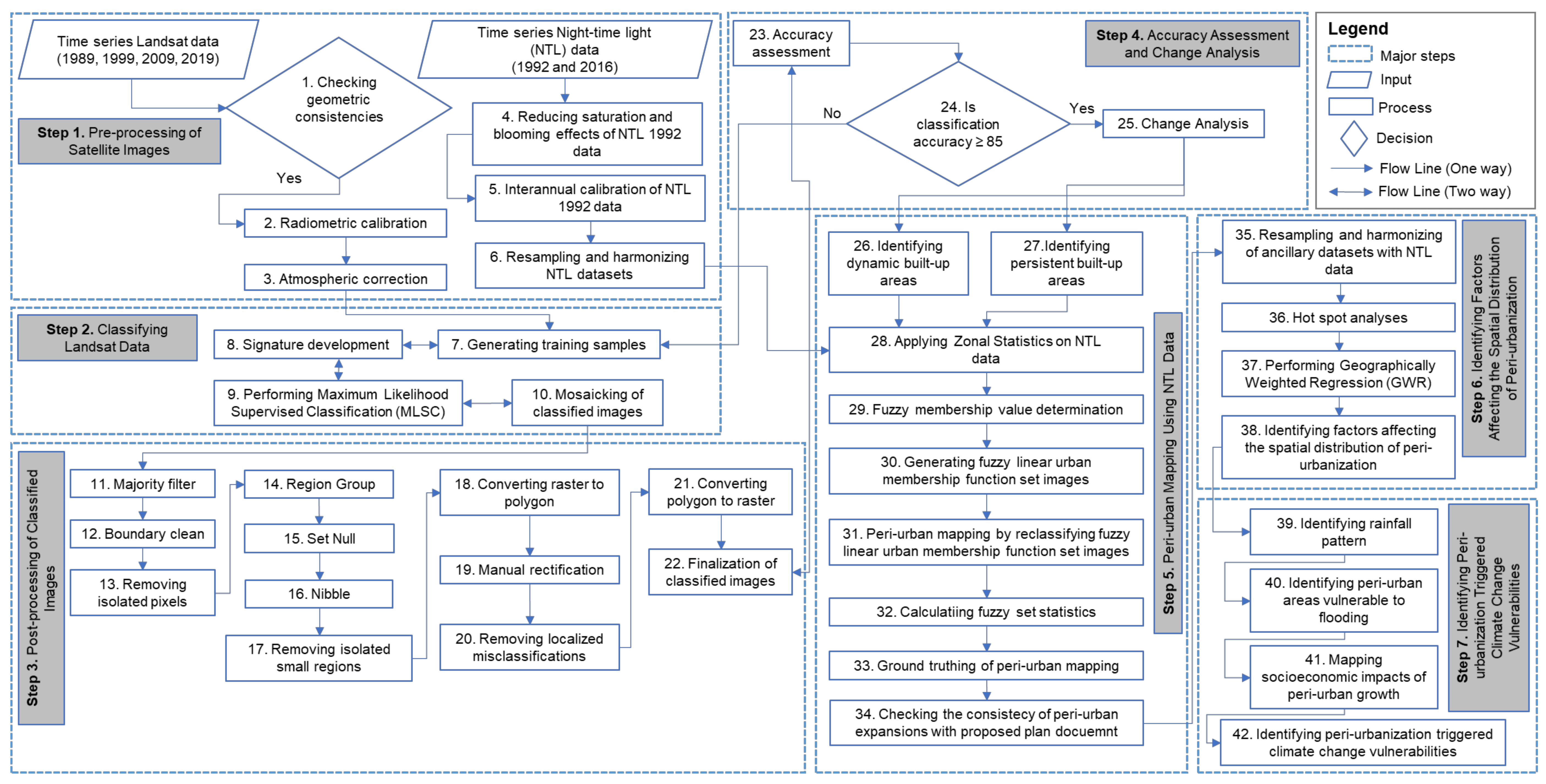
The collected raster datasets and shapefiles were all projected to the universal coordinate system: ‘WGS_1984_UTM_Zone_46N’. Figure 2 illustrates the overall methodology of this study, while the methodological steps are spelled out in the following sub-sections.

2.3.1. Pre-Processing of Satellite Images

Preprocessing of Landsat Data

The collected Landsat images were carefully cross-checked to ensure that all collected images were geometrically corrected. Thus, no image-to-image spatial adjustments were performed thereafter.
Nevertheless, two accompanying Landsat scenes altogether cover the entire boundary of the DMDP area. However, due to the differences in sun angle as well as in the timing and date of image acquisition, the spectral signatures of each scene were notably different than to its counterpart for each corresponding year. Thus, this study avoided image mosaicking before image classification. The radiometric calibration and atmospheric correction of these collected images were performed thereafter in the ENVI platform.

Preprocessing of NTL Data

The NTL DMSP-OLS data inherently have two main problems [46]: (a) saturation and blooming effects, and; (b) inter-annual inconsistency, whereas such problems with the NTL VIIRS data are assumed to be minimal [47]. Hence, in order to perform the spatio-temporal analysis using NTL data, producing a temporarily consistent DMSP-OLS data became necessary.
Reducing saturation and blooming effects of NTL DMSP-OLS 1992 data: In order to reduce the saturation and blooming effects of the NTL DMDP-OLS data of 1992, this study adapted Cao et al.’s [48] self-adjusting model (SEAM).
The SEAM model was first applied in Beijing, China. Considering the compact land use development pattern and high-density sprawl development that are predominantly prevalent both in Dhaka and Beijing [49,50], Dhaka’s urban growth pattern and subsequent night-time light illumination appears to be similar with the corresponding illuminations of Beijing. Thus, the paper utilized this SEAM model for the DMDP area context by using the SEAM’s script coded in MATLAB. In addition, this study chose the SEAM model because it can alleviate the saturation and blooming effects of the NTL DMSP-OLS images without the help of other auxiliary data.
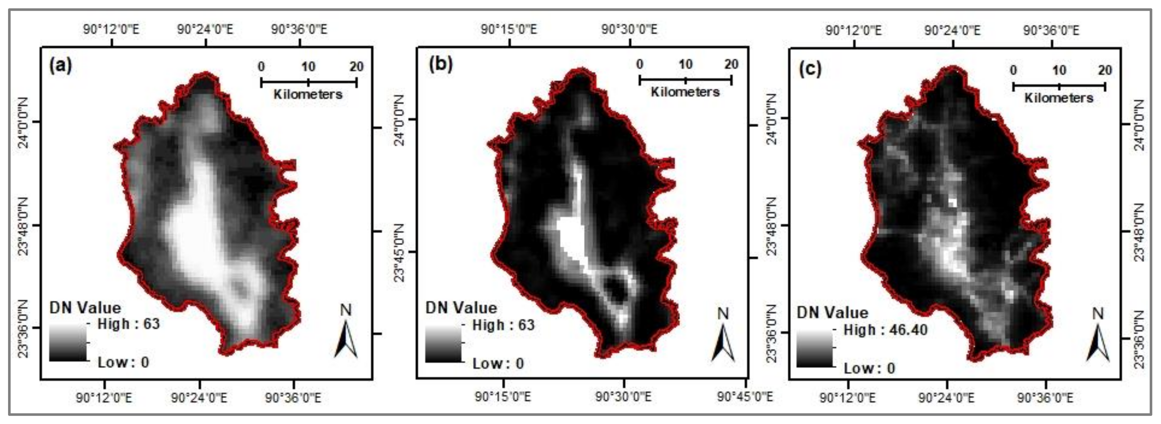
According to the SEAM model, the saturation and blooming effects are estimated by pixel-based regression using pseudo light pixels (PLPs) and their neighboring light sources. These PLPs are selected from the urban edges. The PLPs shown in Figure 3 represent weak brightness (i.e., Digital Number (DN) > 0), but one or more of its eight neighbors are dark (i.e., DN = 0). For each DMSP pixel with DN larger than 0, PLPs are selected within a radius of 150 km.
Interannual Calibration of NTL 1992 data: The SEAM-corrected NTL DMSP-OLS data of 1992 (Figure 4b) were further intercalibrated by using Wu et al.’s [51] study approach. The following equation was applied:
DNc = a X (DNm + 1)b − 1
where DNc = intercalibrated NTL DMSP-OLS image of 1992; DNm = SEAM-corrected NTL DMSP-OLS image of 1992; a = model coefficient = 0.8959; and b = model coefficient = 1.0310. The negative value of the NTL data of 1992 was later set to zero. This way, the NTL DMDP-OLS data of 1992 were made compatible with the NTL VIIRS data of 2016 to carry out spatio-temporal dynamics of peri-urban growth.
Resampling and harmonizing NTL datasets: In the case of selecting the NTL dataset of 2016, this study chose the VIIRS annual average radiance composite vcm-orm-ntl data of 2016, which are cloud-free, outlier removed, stray-light corrected, ephemeral-lights eliminated, and geometrically corrected. Hence, no pre-processing on NTL VIIRS data was performed. These NTL data of 2016 were projected to the WGS_1984_UTM_Zone_46N reference system. The spatial resolution of the projected NTL VIIRS data was 451.52m and radiance values (a.k.a. DN values) within the selected DMDP area were between 0 and 69.86 nanowatts/cm2/sr. In order to bring harmony with the spatial resolution of the NTL DMSP-OLS data of 1992, the NTL data of 2016 were then resampled to 903.04 m spatial resolution by using the ‘bilinear’ resampling technique in the ArcGIS platform (Figure 4c).

2.3.2. Classifying Landsat Data

This study applied the most commonly used maximum likelihood supervised classification (MLSC) technique in the ENVI Platform to classify each selected Landsat image into five land cover categories: (a) bare soil; (b) built-up; (c) vegetation; (d) water body, and; (e) low-land. Other classification techniques—e.g., random forest algorithms, support vector machines, decision tree algorithm—are also popular for classifying remotely-sensed data. However, for classifying Landsat data, in particular, taking appropriate training samples produces more accurate classification outcomes than adapting any specific classification technique itself [52,53]. Given that the MLSC technique is robust and available with any remote sensing software package [54], this study selected this MLSC technique. While applying the MLSC technique, the training samples were repeatedly modified in order to ensure the selection of the most representative fraction for each land cover class for yielding the most accurate classification outcome. Later on, post-classification mosaic for each selected year’s image was performed in order to accommodate the entire boundary of DMDP area within a single classified image frame.

2.3.3. Post-Processing of Classified Images

All classified images were found with ‘salt-and-pepper’ effects and some degree of localized misclassifications—e.g., ‘bare soil’ was misclassified as ‘built-up areas’, and ‘built-up areas’ was misclassified as ‘bare soil’. In addition, in some places, low-density scattered settlements were misclassified as ‘vegetation’ due to the shade of vegetation coverage. Nonetheless, due to the lower resolution of Landsat images, such perceived misclassifications are common with Landsat image classification [53].
Hence, post-processing of classified images became necessary, which was subsequently carried out in the ArcGIS platform. First, in order to remove the ‘salt-and-pepper’ effects—i.e., removing the presence of isolated pixels from classified images, this study employed ‘Majority Filter’ by using the three by three window. Second, the ‘Boundary Clean’ tool was used for smoothening the boundary of land cover classes. Third, for removing the small isolated regions, the study further generalized classified images by sequentially using the ‘Region Group’, ‘Set Null’, and ‘Nibble’ tools. Fourth, the classified raster images were further vectorized in order to manually rectify the localized misclassifications. After manual rectification of localized misclassification, these images were again rasterized to make those images fit for accuracy assessment.

2.3.4. Accuracy Assessment of Classified Images and Change Analysis

The accuracy assessment of classified images was performed in the Google Earth platform. In the case of selecting the number of sampling points for accuracy assessment, if the study area’s coverage is less than 1 million acres and the classified land cover categories are fewer than 12 land cover classes, a minimum of 50 sampling points for each land cover category is recommended [55]. In this regard, the size of the study area was 377,842.53 acres, and the number of classified land cover categories was 5. Thus, the threshold sampling points for this accuracy assessment task were 250. However, the number of sampling points under the stratified random sampling technique is proportional to the area coverage of each land cover class. As some land cover classes (e.g., water body) were too rare, formulation of a minimum of 50 stratified random sampling points for each land cover class was not possible. Finally, a total of 351 random sampling points was generated through stratified random sampling technique in the ArcGIS spatial analyst platform. The image classification process and the corresponding post-processing tasks of classified images as mentioned above were repeatedly done until all classified images were found with a minimum classification accuracy of 85% [56]. Overall classification accuracies of the classified images for 1989, 1999, 2009, and 2019 were 90.00%, 84.90%, 84.90%, and 85.47% with Kappa coefficients of 0.849, 0.778, 0.775, and 0.769, respectively. Finally, post-classification change detection was carried out by using Land Change Modeler (LCM) in the TerrSet Geospatial Monitoring and Modelling platform.

2.3.5. Peri-Urban Mapping Using NTL Data

Recognizing the Fuzzy Characters of Peri-Urban Areas

Peri-urban areas generally start from location proximity to an urban core and continue until a predominantly rural landscape is found. Thus, peri-urban areas, in general, comprise both the characteristics of urban and rural land uses, where some portions of peri-urban areas are more urban, and the remaining factions are more rural. Hence, peri-urban areas significantly possess the characteristics of the fuzzy-set theory—which limits peri-urban areas within a fuzzy membership value of 0 and 1, where ‘0 = predominantly rural’, and ‘1 = predominantly urban’. Consequently, the values between 0 and 1 imply peri-urban areas, where higher membership values (e.g., 0.75) indicate more peri-urban—i.e., inclined to more urban—and lower values (e.g., 0.15) indicates less peri-urban—i.e., inclined to more rural. Henceforth, this study applied the fuzzy membership function to reveal these perceived fuzzy characteristics of peri-urban areas.

Identifying the Suitable Fuzzy Membership Function

This study primarily centered around selecting a suitable fuzzy membership function to reveal the fuzzy characterizes of peri-urban areas. Initially, fuzzy ‘Gaussian’ and ‘Linear’ membership functions on NTL data in the ArcGIS platform were run. By using multiple combinations as input values, it is observed that the fuzzy Linear membership function is more interpretive than the Gaussian one while using NTL data. Thus, this paper chose the fuzzy Linear membership function to map the fuzzy characteristics of peri-urbanization and named this as the ‘fuzzy linear urban membership function’.

Selecting the Membership Value for the Fuzzy Linear Urban Membership Function

In order to determine the minimum and maximum membership values of the fuzzy linear urban membership function, this study first extracted the persistent and dynamic built-up areas. The persistent built-up areas are those which remained unchanged between 1989 and 2019, while the dynamic built-up areas are the landscapes which were converted into built-up surfaces between 1989 and 2019. As peri-urban areas become urbanized over a 20- to 30-year period, the built-up areas showing persistence between 1989 and 2019 were hypothesized to be predominantly urban. Thus, this study assumes that the characteristics of peri-urban areas lie within the dynamic built-up surfaces. Henceforth, this study extracted the areas which were converted into built-up surfaces between 1989 and 2019.
Later on, this study carried out zonal statistics on the NTL datasets of 1992 and 2016 for the areas comprising persistent and dynamic built-up areas individually (Table 2). It is observed that the mean value between these two separate built-up zones is significantly different, while the differences in the maximum values between these two separate zones are not so conspicuous. Thus, the mean value of dynamic built-up areas appears to have significant potential to interpret the peri-urbanization pattern of the DMDP area. Consequently, this study took the ‘minimum value’ and ‘mean value’ as the ‘minimum value’ and ‘maximum value’, respectively, to form the fuzzy linear urban membership function set images in the ArcGIS platform. Any values more than the mean estimate (which was subsequently considered as the ‘maximum value’) indicated predominantly urban areas in the fuzzy linear urban membership function set images.
It is important to mention that this study only used the boundary of dynamic built-up areas in order to derive the membership values for the fuzzy linear urban membership function set images using NTL data. No pixel-to-pixel comparison was performed between 30 m resolution classified Landsat data and 903.04 m resolution NTL data. This way, the difficulty of handling the variations in spatial resolution of these two different image datasets was avoided.

Identification of Peri-Urban Areas within the Fuzzy Linear Urban Membership Function Set Images

The urban core areas were predominantly found within the values of 0.80 to 1.0, while the rural areas were predominantly found within the value range of 0 to 0.10 in the fuzzy linear urban membership function set images. Consequently, peri-urban areas are delimited within the value range of 0.11 to 0.79. Hence, by using these perceived value ranges, the fuzzy linear urban membership function set images of the years 1992 and 2016 are reclassified into three categories (Figure 5): (a) predominantly urban (PURBAN); (b) predominantly rural (PRURAL), and; (c) peri-urban (PU).

Derivation of Fuzzy Set Statistics for the Study Area

This study derived the overall level of urbanization and the degree of fuzziness for the DMDP context. The level of urbanization denotes the mean gross level of membership in the fuzzy linear urban membership function set. The following equation was used to calculate the level of urbanization.
LoU year = i n F year n
where LoU is the the level of urbanization of each corresponding year, and n is the total number of cells in the corresponding fuzzy linear urban membership function set image.
In order to determine the degree of fuzziness, the following equation was used:
DoF year = ( F year F Predominantly   Urban F year ) n
where DoFyear = the degree of fuzziness for each corresponding year, and FPredominantly Urban = fuzzy linear membership function set for predominantly urban areas of each corresponding year, where the minimum and maximum values for the predominantly urban set image were assigned to 0.80 and 1.0 respectively.

2.3.6. Validation of Peri-Urban Mapping

Ground Truthing of Peri-Urban Mapping

In order to determine the accuracy of the peri-urban mapping approach, this study carried out ground-truthing by using 300 stratified random sampling points. Considering the availability of data for the purpose of ground-truthing using the Google Earth platform, the study chose NTL VIIRS data mapping of 2016 for this ground-truthing purpose. Nevertheless, as peri-urbanization is local context-specific, a set of criteria was primarily formulated to distinguish the areas which are predominantly urban, peri-urban, or predominantly rural for the context of the DMDP area (Table 3). Later on, a ground-truthing exercise was performed in the Google Earth platform and a confusion matrix was formed thereafter to derive the accuracy of the peri-urban mapping exercise of 2016.

Checking the Consistency of Peri-Urban Expansions with the Proposed Plan Documents

In order to determine the changes in peri-urban growth corresponding to the proposed changes as stipulated in the DMDP’s City Region Development Project (CRDP) 2015–2035, this study compared the NTL VIIRS data mapping of 2016 with the proposed land use zones of CRDP 2015–2035.

2.3.7. Identifying Factors Affecting the Spatial Distribution of Peri-Urbanization

Pre-Processing of Ancillary Datasets

The collected raster datasets on demography, the average likelihood of poverty (ALP) and standard deviation of the average likelihood of poverty (ALP), and the continuous surface elevation dataset generated for the DMDP context were all resampled to 903.04 m spatial resolution (by using ‘bilinear’ resampling technique in the ArcGIS platform) in order to obtain consistency with the NTL data-driven peri-urban mapping for comparative analysis. This study considers the standard deviation of the average likelihood of poverty (ALP) as a proxy variable of social stratification.

Identification of Statistically Significant Hot Spots for Interpreting Peri-Urbanization

In order to reveal whether the spatial distribution of population growth, the standard deviation of the average likelihood of poverty (ALP), elevation, and corresponding changes in the spatial distribution of peri-urbanization is clustered, random, or dispersed, the spatial autocorrelation was carried out to derive the Global Moran’s I statistic. The positive Moran’s Index implies a tendency towards spatial clustering, while the negative value of Moran’s Index insinuates a tendency towards spatial dispersion. Based on the outcome of the spatial autocorrelation against each parameter as mentioned above, the null hypothesis ‘spatial distribution of a given parameter is normally distributed’ was tested.
Afterwards, hotspot analysis was carried out to compute the Getis-Ord Gi* in order to measure the intensity of such perceived clustering. While identifying the Getis-Ord Gi* statistic, a False Discovery Rate (FDR) correction was applied in order to resolve the issues of spatial dependency and multiple testing. Regardless of whether the z-score is positive or negative, a higher z-score value implies more spatial clustering. A positive z-score value indicates clustering of hot spots, while a z-score with a negative value indicates clustering of cold spots, and a z-score near zero implies clustering is ‘not significant’, meaning that no apparent spatial clustering is evident.

Performing Geographically Weighted Regression

The Geographically Weighted Regression (GWR) was carried out in order to reveal how peri-urbanization is interpreted as a response variable to the spatial distribution of population growth, the standard deviation of the average likelihood of poverty (ALP), and elevation pattern for the DMDP context.

2.3.8. Identifying Peri-Urbanization Triggered Climate Change Vulnerabilities

Identifying Rainfall Pattern of the Study Area

The daily rainfall data from 2000 to 2018 (collected from the Bangladesh Water Development Board) were used to derive the statistics on total annual rainfall, annual monsoon rainfall, and annual non-monsoon rainfall. Each year’s rainfall from May to September was considered as the ‘annual monsoon rainfall’, and the rainfall of the remaining months for each year was considered as the ‘annual non-monsoon rainfall’.

Identification of Peri-Urban Growth Pockets Vulnerable to Flooding

The data on DMDP’s flood plain area (collected from the RAJUK) were superimposed on NTL VIIRS data mapping of 2016 in order to find out the peri-urban growth pockets vulnerable to flooding.

Mapping the Socioeconomic Impacts of Peri-Urban Growth

The demographic data for the years 2001, 2016, and 2020, the average likelihood of poverty (ALP) and the standard deviation of the average likelihood of poverty (ALP) for the year 2013 for the DMDP context were all analyzed and compared with the NTL VIIRS data mapping of 2016 in order to illustrate how the changes in the spatial distribution of demography and the standard deviation of ALP correspond to the changes in peri-urban growth.

3. Results

3.1. Changes in Land Cover

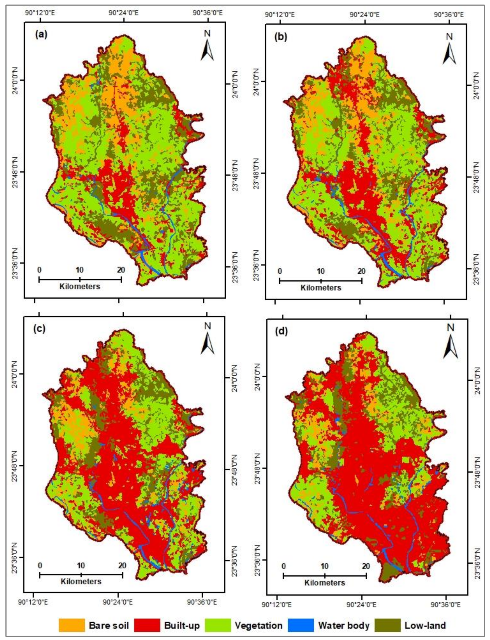
The classified images are presented in Figure 6, while the aerial statistics of those classified images are presented in Table 4.
The results find that except for built-up areas, the remaining land cover categories declined over time. While the highest decline of 22.18% is observed in the vegetation category, the ‘bare soil’ and ‘low-land’ categories also demonstrate a significant decline over this 30-year period. Thus, the losses in bare soil, vegetation, and lowlands contributed altogether to the development of built-up areas over time. Consequently, built-up areas quadrupled over time and constituted more than half (i.e., 52%) of the DMDP area in 2019, whereas bare soil and vegetation were more than halved within this 30-year period. Earlier studies also found a similar growth trend for bare soil, built-up, vegetation, and lowland areas (e.g., [57,58,59]).
In addition, all land cover categories (except water body) demonstrate an exponential growth/decline trend with strong coefficient of determination values of R2.
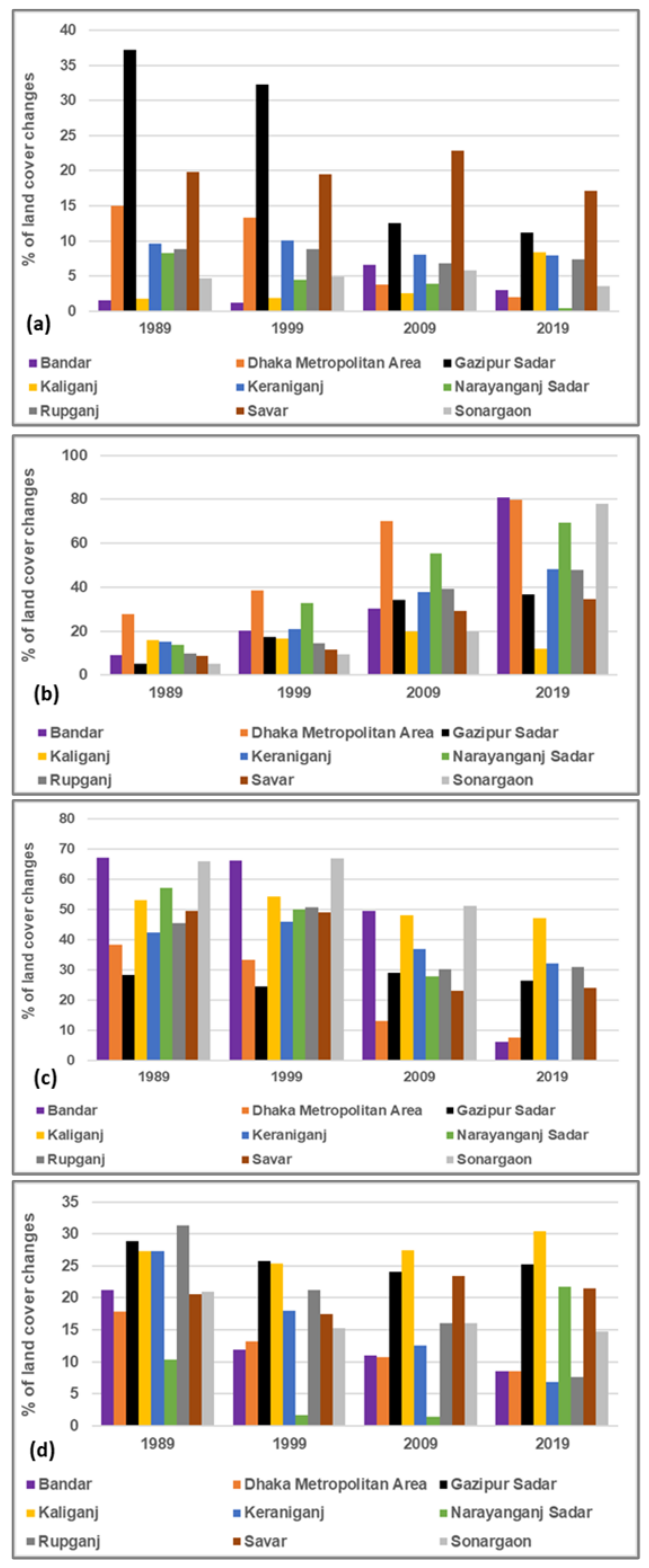
In the case of sub-district-wise net changes in bare soil, Gazipur Sadar encountered the highest decline (i.e., 26%) in bare soil, followed by the Dhaka Metropolitan Area (DMA), and Narayanganj Sadar by 13% and 8%, respectively, between 1989 and 2019 (Figure 7). While sub-districts predominantly lost bare soil over time, Kaliganj presented an increase of 7% for bare soil within this 30-year period. On the contrary, all sub-districts encountered significant losses in vegetation. As for the case of built-up areas, all sub-districts except for Kaliganj demonstrated significant increases over time, while built-up areas of Kaliganj declined by 4% between 1989 and 2019.

3.2. Changes in Peri-Urban Boundary

The aerial statistics of peri-urban growth has been presented in Table 5, while the peri-urban mapping has been depicted in Figure 8. The analysis reveals that for the DMDP context, predominantly urban areas remained nearly unchanged over time, while the major changes occurred in transitioning predominantly rural areas into peri-urban areas (Table 5). Thus, major development within the DMDP context predominantly took place in the form of peri-urbanization.
The level of urbanization within the predominantly urban areas category was 0.94 and 0.96 in 1992 and 2016, respectively. Thus, predominantly urban areas had undergone the highest level of urbanization within these 24 years (1992–2016), followed by peri-urban areas and predominantly rural areas. Nevertheless, in terms of the level of urbanization, predominantly urban areas demonstrated an increase of 2.13% only, which resulted in an increase of 71.43% in the degree of fuzziness in 2016 from the base year estimate of 1992. Such a finding reveals that along with the pace of urbanization, a less articulated pattern of urban land use practices becomes more evident.
In addition, the level of urbanization within the predominantly rural areas category demonstrates the same thing, while the degree of fuzziness within this zone is 1.00 in 1992 and 2016, meaning the land use practices embraced an unclear pattern in distinguishing whether the areas are predominantly rural or urban.
Furthermore, predominantly rural areas and peri-urban areas both demonstrated an increase of 33.33% in the level of urbanization in 2016. However, while unquestionably rural areas demonstrated persistence in encountering the highest degree of fuzziness in 1992 and 2016, peri-urban areas showed a slight decline of 4.08% in 2016, implying a nominal improvement in embracing articulated land use practices within peri-urban areas.
In the case of the sub-district-wise level of urbanization and degree of fuzziness, with the correlation coefficients of (-)0.97 and (-)0.95, respectively, for the years 1992 and 2016, the result reveals that the degree of fuzziness is inversely correlated to the level of urbanization, with Bandar being an exception (Figure 9). The Bandar sub-district encountered the highest increase in the rate of the level of urbanization (i.e., 277%) and experienced a reduction in the degree of fuzziness, from 0.93 to 0.65 in 2016. Such a finding implies that scattered urban development in Bandar has been further consolidated through increased urbanization, resulting in a decrease in the degree of fuzziness thereafter. The Dhaka Metropolitan Area (DMA), and Narayanganj Sadar continued the higher level of urbanization both in 1992 and 2016, and hence scored the lowest in terms of the degree of fuzziness.
The remaining sub-districts underwent less urbanization and encountered more fuzziness, meaning that an intensified unarticulated peri-urbanization predominantly took place within these (remaining) sub-districts.

3.3. Validation of Peri-Urban Mapping

3.3.1. Ground-Truthing of Peri-Urban Mapping

The spatial distribution of the ground-truthing points generated through the stratified random sampling technique is presented in Figure 10, while the confusion matrix of this ground-truthing exercise is given in Table 6. With a Kappa coefficient of 0.75, the ground-truthing exercise yields an overall accuracy of 86%.

3.3.2. Consistency of Peri-urban Expansions with the Proposed Plan Documents

The City Region Development Plan (CRDP) proposed land use zone of 2015–2035 was superimposed over the NTL VIIRS data mapping of 2016 in order to cross-check how the adapted peri-urban mapping approach fits with the proposed land use zoning for the DMDP area.
The CRDP’s 2015–2035 proposed land use zones comprise eight broad land use categories (Figure 11). The analysis reveals that the mixed-use zone (55%) and agricultural zone (29%) are the two most dominant proposed land use zones in the DMDP area, which altogether account for 84% of the DMDP’s area coverage (Table 7).
According to the NTL VIIRS data mapping of 2016, predominantly rural areas comprise 11% of the DMDP area, out of which the CRDP’s 2015–2035 proposed agricultural zone and mixed use (i.e., a blend of residential, commercial, and general industrial areas) zone altogether comprise around 10%.
Similarly, in an aggregate, peri-urban areas comprise around 58% of the DMDP’s area, whereas mixed use zones (28.10%) and agricultural zones (21.87%) altogether comprise around 50% of the DMDP’s peri-urban area. Thus, peri-urban areas are proposed to accommodate around three fourths of the DMDP’s proposed agricultural areas and more than half of the proposed mixed-use zone. Predominantly urban areas are proposed to be dominated by mixed use zones which comprise around two fifths of the proposed mixed-use zone areas.
Among the other proposed land use zones, institutional zones comprise around 4% of the DMDP’s area, and comprise 2.61% and 1.33% of the predominantly urban and peri-urban areas, respectively. In addition, more than three fourths of the DMDP’s proposed heavy industrial zone is located in predominantly urban areas. Meanwhile, among the total proposed forest areas, nearly three fourths of the proposed forest zones are located in peri-urban areas and the remaining portion was proposed to be accommodated by predominantly rural areas.
The analysis reveals that the proposed forest areas are observed as having the lowest values for LoU and the highest values for DoF (Figure 12). Contrariwise, the proposed heavy industrial zone appeared to be the most urbanized in terms of LoU, and hence had the lowest values for DoF. Apparently, heavy industrial zones are proposed based on strict policy control, and hence spontaneous development of these areas are not possible, resulting in an articulated land use pattern of these areas. Meanwhile, forested areas are spontaneous natural growth zones, and hence were observed as having the highest DoF.
In addition, in the case of each subdistrict, the higher the LoU, lower the level of DoF in each proposed land use zone is (Figure 13). The Kaliganj sub-district, with the lowest LoU and an absolute DoF value of 1.0, provokes an immediate land use intervention by the city authorities (Figure 13d). Other sub-districts with higher DoF include Gazipur, Keraniganj, Rupganj, Sonargaon, and Savar. These areas are predominantly located in peri-urban areas, meaning that peri-urban growth appears to be dominated by unarticulated land use patterns.
Such general findings are also evident in the sub-district-wise LoU and DoF calculations that were derived from the NTL VIIRS data mapping of 2016 (Figure 9). Thus, it can be deduced that the proposed NTL data mapping exercise of 2016 yields substantive outcomes in distinguishing predominantly rural, peri-urban, and predominantly urban areas.

3.4. Factors Affecting the Spatial Distribution of Peri-Urbanization

3.4.1. Identification of Statistically Significant Hot Spots for Interpreting Peri-Urbanization

Hotspots of Population Growth

In the DMDP area, a highly statistically significant (Moran’s Index: 0.69, p-value = 0, and hence the null hypothesis ‘spatial distribution of the population is normally distributed’ was rejected) cluster pattern of population growth is evident. The hot spots of population increase are found predominantly in the Gazipur Sadar areas (Figure 14a), which bolsters the earlier findings on Gazipur Sadar’s supremacy in attainting the highest rate of population growth. However, Savar areas are prevalent with both hot spots and cold spots. Indeed, the northern part of Savar in proximity to the Gazipur Sadar areas is observed as having hot spots, whereas the southern part of Savar in proximity to the Dhaka Metropolitan area is found to have the cold spots for population growth. As Savar is found to have both cold and hot spots of population growth, the aggregate growth rate of population in Savar does not appear to be higher than its contemporaries, although the earlier findings claim that Savar is the most peri-urbanized sub-district for this study.

Hotspots Mapping of the Standard Deviation of the Average Likelihood of Poverty

The hotspots mapping exercise on the standard deviation of the average likelihood of poverty (ALP) demonstrates a highly statistically significant clustering pattern (Moran’s Index = 0.78 and p-value = 0, and hence the null hypothesis ‘spatial distribution of poverty deviation is normally distributed’ was rejected). However, in this regard, hot spots are predominantly confined within the Dhaka Metropolitan Area while the cold spots are predominantly observed near the eastern periphery of the Dhaka Metropolitan Area, which enjoins Rupganj, Sonargaon, and Kaliganj sub-districts (Figure 14b). Thus, the spatial distribution of the standard deviation of ALP hot-spot mapping exercise does not appear to be commensurate with the hot spot mapping of the population growth pattern.

Hotspots of Elevation Pattern

A statistically significant (Moran’s Index: 0.56, p-value = 0, and hence the null hypothesis ‘spatial distribution of elevation pattern is normally distributed’ was rejected) clustering pattern is dominant in the spatial distribution of elevation for the DMDP area. The hot spots (i.e., areas with higher elevation) are predominantly concentrated in the Gazipur Sadar and Savar sub-districts—i.e., the areas which underwent the highest peri-urbanization (Figure 14c).

Hotspots of Peri-Urbanization

This study used the NTL VIIRS data mapping of 2016 in determining the spatial distribution of hotspots for peri-urbanization (Figure 14d). The Moran’s Index was computed as (+)0.90 with a z-score value of 54.51 and p-value of 0. Thus, the null hypothesis ‘spatial distribution of peri-urbanization pattern is normally distributed’ was rejected, implying that the spatial distribution of the fuzzy linear urban membership function set image of 2016 (i.e., NTL VIIRS data mapping of 2016) demonstrates a highly significant clustering pattern.
The analysis reveals that hot spots are predominantly urban, whereas the cold spots are predominantly rural (Figure 14d). On the contrary, the areas which are not statistically significant in the fuzzy linear urban membership function set image of 2016 are predominantly peri-urban. Indeed, peri-urban areas which are neither urban or rural seem to possess more fuzzy characteristics, which in turn lead to them to be statistically insignificant.

3.4.2. Carrying out Geographically Weighted Regression for Interpreting Peri-Urbanization

The findings from hot spot analysis reveal that the spatial distribution of peri-urban hot spots mapping is more linked to the corresponding distribution pattern of elevation and the growth of population. Thus, in order to illustrate how such perceived peri-urbanization of the DMDP area varies across space corresponding to the changes in elevation and population growth pattern, Geographically Weighted Regression (GWR) was carried out. The adjusted R2 value of the GWR model was 0.87, indicating that peri-urbanization is predominantly linked to higher elevation and higher population growth rate. Meanwhile, the R2 value of the GWR model was 0.63 when peri-urbanization was interpreted as a response variable of elevation, population growth rate, and the standard deviation of ALP. Thus, when the standard deviation of ALP is omitted, the GWR model interpreting DMDP’s peri-urbanization produces a better outcome, meaning that peri-urbanization does not necessarily mean an over concentration of poverty in the city’s outskirts. Instated, such concentration is predominantly driven by the land scarcity in the city’s core and an unleased influx of population to the capital city Dhaka.

3.5. Identifying Peri-Urbanization Triggered Climate Change Vulnerabilities

3.5.1. Identifying Rainfall Pattern of the Study Area

The annual rainfall pattern of the DMDP area is presented in Figure 15. The analysis reveals that from 2000 to 2018, total annual rainfall in the DMDP area ranged from 818.1 (in 2010) to 2873 mm (in 2017), with an annual average rainfall of 1824.91 mm within this 18-year period. In addition, it was calculated that the annual average rainfall in the monsoon—which lasts from September to May—comprised exactly 80% of the total annual rainfall within this 18-year period.
Surprisingly, in 2012, the DMDP area had the lowest annual monsoon rainfall percentage of 67.72%, whereas in the following year (i.e., in the year 2013), the percentage of annual monsoon rainfall was the highest, at 91.30%. In addition, this rainfall pattern does not follow any significant growth trend over time. For example, although the highest annual rainfall occurred in the year 2017, annual monsoon rain within this year was 73.41%, which is below the annual average percentage of monsoon rainfall (i.e., 80%), whereas the highest annual rainfall in the non-monsoon period was observed in 2017.
However, this finding does not simplify with certainty that an occurrence of more rainfall events in the monsoon is linked with less rainfall in the non-monsoon period and vice versa, as the correlation coefficient of the rainfall pattern between the monsoon and non-monsoon period is 0.44 (which is not very strong), meaning that abrupt rainfall in the DMDP area has gradually become common. Consequently, events of frequent flooding due to heavy rainfall often occur in the DMDP area.

3.5.2. Identification of Peri-Urban Growth Pockets Vulnerable to Flooding

In general, DMDP is a flood-prone area. However, the northern part of the DMDP is in higher elevation, and is therefore comparatively less flood-prone (Figure 16). Thus, higher population concentration and subsequent peri-urbanization is observed in the areas with higher elevation, which are predominantly concentrated in the Gazipur Sadar and Savar areas. The analysis reveals that around 44% of total peri-urban areas are located within the flood plain area, while such percentage distribution for predominantly rural and urban areas is 35% and 33%, respectively, meaning that peri-urban areas are most vulnerable to frequent flooding. Such findings are relevant to Dewan et al.’s [61] study, who claimed that the DMDP’s peri-urban areas are moderately to highly vulnerable to annual flooding.

3.5.3. Mapping Socioeconomic Impacts of Peri-Urban Growth

Changes in Demography

The spatial distribution of population predominantly is concentrated within the Dhaka Metropolitan Area (DMA), Narayanganj Sadar, and along the Dhaka-Mymensingh and Tangail-Joydevpur Highways of the Gazipur Sadar area (Figure 17). Apparently, the spatial changes in demography between 2001 and 2016 are quite conspicuous, whereas such changes between 2016 and 2020 appear to be quite similar.
In addition, the percentage distribution of population between predominantly rural areas, peri-urban areas, and predominantly urban areas remained almost equal over time, whereas the density of population nearly doubled within this 19-year period (Table 8). Thus, this study finds a perpetual increase in growth rate of population over time for the DMDP context. Although the density of population in DMDP’s predominantly urban areas is unparalleled compared to the rest of the world, the population density of even DMDP’s predominantly rural areas is much higher than some of the urban areas’ population density of the developed world. For example, a country like Australia, which comprises more than 50 times larger area coverage than Bangladesh, has an urban area population density of 903 persons/km2 [41].
Nevertheless, the population density of the Dhaka City Corporation (DCC) area is 52,000 persons/km2 [40], whereas the estimated 2020 population density for predominantly urban areas is 31,666. Indeed, predominantly urban areas of 2016 cover an area of 478 km2, whereas the area coverage of DCC is 134 km2. Thus, NTL VIIRS 2016 data estimated that predominantly urban areas are more than 3.5 times larger than the DCC’s area coverage. Hence, such perceived lower population density in predominantly urban areas is likely, as DMDP’s predominantly urban areas extend far beyond the jurisdiction of the DCC boundary.

Population Densification and Peri-Urban Growth

In general, predominantly urban areas have a relatively lower growth of population, while predominantly rural areas and peri-urban areas have higher growth rates of population.
Figure 18a illustrates the spatial changes in peri-urban mapping between 1992 and 2016, while the aerial statistics of these changes are presented in Figure 18b. The analysis reveals that the highest percentage distribution lies in the peri-urban areas category, which covers more than one-third of the DMDP’s area. Surprisingly, in terms of spatial changes between the areas of predominantly rural, peri-urban, and predominantly urban, around two thirds (i.e., 63%) of the DMDP area demonstrated persistence over time. However, the third and fourth highest categories are the transition of predominantly rural areas to peri-urban areas and the transition of peri-urban areas to predominantly urban areas, constituting 18.25% and 7.08% of the area, respectively.
In terms of aggregate population growth rate that occurred between 2001 and 2020, the analyses reveal that persistent predominantly rural areas encountered the highest pressure of population growth by around 135%—i.e., 7.10% per year. Among the areas which remained persistent over time, predominantly urban areas exhibited the lowest population growth rate. The second highest growth rate of population was observed in the ‘peri-urban to predominantly urban’ areas category by 125.91%, implying a sequential transition of ‘predominantly rural areas to peri-urban areas’ and the subsequent transition of ‘peri-urban areas to predominantly urban’ areas.
Nevertheless, the areas demonstrating the transition of peri-urban to predominantly rural shows the third highest concentration of population growth by 113.05%, which predominantly occurred near the persistent predominantly rural areas of Kaliganj sub-district. Such a finding, in fact, is not unlikely as these persistent predominantly rural areas conglomerate the highest percentage of population growth between 2001 and 2020.
Surprisingly, an unusual transition titled ‘predominantly urban to predominantly rural’ is observed in the Narayanganj Sadar area which accounted for a negative growth rate of population. These areas of negative population growth are located in the highly flood prone area of the Dhaleshwari River’s catchment, and hence frequent flooding displaces many people from this specific chunk of landscapes.
In terms of the sub-district-wise population growth rate, the Gazipur Sadar area encountered the highest rate of population increase with a larger margin than its contemporaries (Figure 18c). The areas—i.e., Kaliganj, Keraniganj, Rupganj, which are predominantly peri-urban or predominantly rural in type—have nearly the same rate of population growth in dynamic and persistent areas. Meanwhile, the two most urbanized areas—i.e., the Dhaka Metropolitan Area (DMA), and Narayanganj Sadar area—are observed as having the lowest rate of population increase. In addition, the population growth difference between persistent and dynamic areas is also found to be relatively higher in the Narayanganj Sadar and Dhaka Metropolitan Areas. However, the population growth rate in dynamic areas is relatively lower in each sub-district compared to the corresponding population growth rate of persistent areas, with Savar being an exception. The Savar sub-district possesses the largest chunk of landscapes which have been converted into peri-urban areas from predominantly rural, implying that Savar is the most peri-urbanized sub-district of this study. Such findings reveal that peri-urbanization is more linked to population increase in dynamic areas. Thus, while the Dhaka Metropolitan Area and Narayanganj Sadar area have extremely limited scope for peri-urbanization, the nearby sub-districts are potential areas for such peri-urban expansions.

Poverty and Peri-Urban Growth

The average likelihood of poverty (ALP) is more dominant in the Kaliganj sub-district and trickles down to its nearby sub-districts of the Gazipur Sadar and Rupganj (Figure 19a), whereas such poverty concentration is relatively lower in the Dhaka Metropolitan Area, Narayanganj Sadar, and Bandar areas. The above-mentioned Dhaka Metropolitan Area, Narayanganj Sadar, and Bandar areas are also observed as having higher population growth difference between dynamic areas and persistent areas, meaning that the influx of poor migrants is predominantly confined to the dynamic land parcels of Kaliganj and its nearby areas.
However, the standard deviation mapping of the average likelihood of poverty (ALP) depicts that the DMDP area is inflicted with higher variation in poverty concentration, that ranges from 2.8 to 6.5 (Figure 19b). Although a higher concentration of poverty is found in the Kaliganj, Rupganj and Gazipur Sadar areas, the Dhaka Metropolitan Area is observed with the highest deviation in the average likelihood of poverty (ALP), meaning that inequalities in social stratification within predominantly urban areas are comparatively higher.
Most parts of the Dhaka Metropolitan Area and Narayanganj Sadar area are already predominantly urbanized, while, through increasing peri-urbanization, the Savar sub-district is in the queue to be predominantly urbanized shortly. Consequently, the Dhaka Metropolitan Area, Narayanganj Sadar area, and Savar are derived as the sub-districts of higher poverty deviation (Figure 19d). Thus, the deviation in poverty concentration appears to be correlated with urbanization. For example, the Dhaka Metropolitan Area, as the most urbanized, ended up with the highest poverty deviation. Such a deviation in poverty intensification can further be illustrated by the abundance of slum settlements which are scattered throughout the DMDP area (Figure 19b).

4. Discussion

4.1. Factors Affecting Peri-Urbanization

While the horizontal expansion of the DMDP area is remarkably constrained by the unavailability of flood-free landscapes, the northern part of the DMDP area encountered the highest growth rate of population and subsequent peri-urbanization pressure. The DMDP’s northern periphery, in general, lies at a higher elevation and is therefore naturally free from seasonal flooding. Thus, the findings reveal that peri-urbanization for the DMDP context is interpreted as an interaction space of elevation and population growth rate. Consequently, in-migration of the population to the capital city Dhaka plays a significant role for this perceived peri-urbanization. Yet, such an in-migration pattern is profoundly interlinked to the unique socio-economic settings of this country.
For example, the Dhaka’s share of the national gross domestic product (GDP) is USD 162 billion (i.e., 40%) [64], implying a heavily inclined concentration of economic activities towards the capital city Dhaka. Consequently, Dhaka is disproportionately equipped with nearly one third (i.e., 31.8%) of the country’s total employment [21]. In general, Bangladesh’s economic base is predominantly agricultural (i.e., 49%), and 45% of the country’s labor force primarily relies on agriculture for employment [65]. In addition, 84% of the rural population directly or indirectly depends on agriculture [66]. The disproportionate growth of agriculture-based industries coupled with the adaption of more efficient farming technologies triggers an exodus of surplus agricultural laborers to the capital city Dhaka [60]. Consequently, 63% of Dhaka’s population growth is due to the rural–urban migration [67].
The majority of the migrants predominantly rely on the informal sector. Subsequently, the informal sector accounts for 84.30% of Dhaka’s total employed population [21]. Thus, anticipating the social changes with response to economic growth becomes more difficult. Consequently, the task of addressing actual spatial growth pattern and accommodating informal economics become highly challenging.
In addition, Dhaka’s per capita GDP is around 3 times higher than the national average. If Dhaka were an independent nation, Dhaka’s gross GDP individually would stand as the 50th largest economy in the world. Consequently, excessive agglomeration of the capital city-centered development paradigm makes the DMDP’s peri-urban growth highly unpredictable and challenging. Thus, DMDP’s physical growth predominantly implies a more densified peri-urban growth which agglomerates overestimated population with inadequate infrastructural supports. The scarcity of resources further hinders the timely upgrading of supporting infrastructures and provisions—e.g., land use–transport integration [68,69], utilities, and employment. This way, policymakers and planners are severely obstructed to enhance a planned development in their peripheries.

4.2. Implications for Growth Management and Natural Hazards

Bangladesh is one of the most vulnerable countries to climate change’s impact. Such impacts are already evident, as climate change-induced flooding—e.g., river flooding and storm water flooding—often strikes in the DMDP area [25]. Most parts of the predominantly urban areas (i.e., around 67%) are considered to be free from river flooding because of the proposed protective embankments, which surround them [60]. Nevertheless, the construction of the DMDP Urban Area Plan (1995–2005) proposed an eastern embankment which as yet remains incomplete. In addition, the portion of predominantly urban areas—that is considered to be flood-free—severely lack an efficient drainage system [70]. The analysis reveals that the DMDP’s rainfall pattern from 2000 to 2018 is rather abrupt. Thus, heavy rainfall often happens, resulting in frequent storm water flooding during each year irrespective of the monsoon. Such a finding is also evident in other studies [25].
Nevertheless, due to the proximity to the nearby river, the remaining 23% of predominantly urban areas seem to be highly vulnerable to river flooding. The low-income people predominantly live in slums, and the spatial distribution of slums is scattered throughout predominantly urban areas. In addition, 80% of these slums are built on privately owned land and hence pose considerable institutional challenges in providing the basic urban facilities [30]—e.g., water supply, sanitation, sewerage, drainage, and electricity—in these slum-inflicted areas. On that very point, Baker [30] estimated that slum areas within a proximity of 50 m to nearby rivers accommodate around 76,000 households those are at high risk of being frequently river flooded. Such river flooding usually occurs with a return period of every 10 to 40 years [71].
However, despite the geographical limitations to support further physical growth, Dhaka’s unleased population growth is not hindered by geographical limitations at all. For example, the analysis reveals that within these 19 years (2001–2020), the DMDP’s population has increased at a rate of 0.5 million/year. Although the urban population as yet comprises less than 37.41% of the nation’s population [72], such a portion reaches nearly 80% for the DMDP context. Nevertheless, the reported estimation of DMDP’s annual population growth rate is 0.10 million/year higher than the earlier estimation by the World Bank [32]. Nonetheless, from 2001 to 2020, the DMDP’s population has increased at an annual growth rate of 4.53%. Such perceived growth rate in the population is much higher than the national average. For example, between 2000 and 2019, the national annual population growth rate was derived as 1.5% [73].
In terms of population size, Dhaka has secured the 19th position globally among the top 20 megacities, but stands first with a large margin in terms of the urban population density of 33,878 persons/km2 [41]. Among the top 20 megacities, only six have constantly experienced a population growth rate of more than 3% over the last 20 years [74]. Hence, the reported rate of DMDP’s population growth is much higher than its contemporaries.
Consequently, due to an unabated growth in the DMDP’s population, higher population concentration is also observed in the north-eastern periphery of the DMDP area (i.e., Rupganj and Kaliganj), which are predominantly flood-prone. In addition, these two areas are the hot spots of poverty with a lower standard deviation in the average likelihood of poverty index, meaning that these two areas predominantly accommodate the poorest portion of the DMDP’s area. Thus, it can be inferred that poverty is forcing the poor migrants to live in these flood-prone areas. This way, the majority of the in-migrants, which also comprise climate migrants [75], are redundantly exposed to this climate change-induced frequent flooding. Such a finding poses a grave concern and brings forth the issue of climate justice for further consideration. On that very point, Ahsan [76] urged the adoption of area-specific growth policies in securing the basic rights for climate migrants of Bangladesh. Similarly, developing sound climate change mitigation policies is deemed critical to minimize climate migrant numbers across the globe [77].
Furthermore, this unleashed population influx to the capital city Dhaka worsens the prevailing water scarcity at large. For example, in 2005, the Dhaka Water Supply and Sanitation Authority (DWASA) was able to manage 1.6 mm3/day groundwater extraction at maximum against the minimum demand of 2.1 mm3/day [78]. In addition, since 1986, the DMDP’s groundwater table has been depleted at a rate of 2 m/year [78]. While the DMDP area is suffering from evident water scarcity, the gradual groundwater depletion coupled with the unprecedented population growth further exacerbates this shortfall.
Nonetheless, due to the prevalence of wetlands, small water bodies, canals, and rivers, the groundwater level is relatively higher in the peripheral areas than the central part of the DMDP area. Unfortunately, peri-urbanization is predominantly taking place in the northern and north-eastern peripheries of the DMDP area, which are the hotspots of industrial clusters and agglomerate more than 2000 ready-made garments (RMG) industries [79]. This RMG sector individually has contributed to 11.17% of the total GDP and makes Bangladesh the second-largest global exporter in the RMG sector [31]. The economic growth of this country is enormously linked to the development of this RMG sector [80]. Hence, the country’s RMG sector possesses great potential to grow further.
Nevertheless, this RMG sector heavily relies on groundwater extraction, because surface water is not available throughout the year. Thus, over-dependence on groundwater extraction coupled with the increased peri-urbanization pose significant environmental threats to these peri-urban growth pockets including land subsidence, increased earthquake vulnerability, and ecosystem degradation.

5. Conclusions

Although managing urban growth based on a demarcated peri-urban growth boundary as yet remains rarely practiced, explicitly defined peri-urban growth pockets appear to be a facilitating tool for promoting more rationalized land use practices in the periphery. Particularly in the context of developing countries, where rampant peri-urbanization frequently occurs, quantifying the magnitude and degree of fuzziness of peri-urban land parcels facilitates policymakers in identifying the areas with more urbanities and higher transition potentials. This way, policymakers and planners will be well equipped in dealing with the dual characteristics (i.e., urban or rural) of peri-urban areas and resultant growth directions, and thereby to identify priority areas for immediate intervention.
Heikkila et al. [81] first recognized the fuzzy characteristics of peri-urban areas, and statistically quantified the level of urbanization and degree of fuzziness in detecting the urban growth pattern of Ningbo, China by using Landsat data. However, they did not map the spatial distribution of peri-urban areas at all, whereas this paper demarcated the spatial distribution of peri-urban growth pockets by unveiling the fuzzy characteristics of peri-urban areas. In doing so, this study developed fuzzy linear urban membership function set images using NTL data.
According to the findings of Mortoja et al.’s [20] study, few studies used NTL data for peri-urban demarcation (e.g., [82,83,84,85]). While all the studies as mentioned above used the crisp values of NTL data, none of the studies, to date, investigated the potential of NTL data in unveiling the fuzzy characteristics of peri-urban areas. In addition, the conventional methodological approaches—which utilized the crisp values of NTL data for peri-urban demarcation—are claimed to be suitable to demarcate peri-urban areas at the national/global level only. Meanwhile, the ground-truthing outcome on NTL VIIRS data mapping of 2016 implies that the methodological approach reported in this study also appears to be a good fit at the regional level. Thus, quantifying the fuzzy characteristics of peri-urban areas and translating those findings into demarcating peri-urban growth pockets using NTL data provides a strong theoretical basis for this study.
Nevertheless, this study did not test other peri-urban demarcation approaches. Hence, how the methodological approach reported in this study prevails over others in terms of accuracy cannot be determined. However, the adapted methodological approach provides an easy way of demarcating peri-urban areas by using the readily available datasets at hand, which in turn facilitates prompt executions of peri-urban growth decisions.
In addition, this study explores how peri-urbanization is interpreted as an interaction space of population growth, poverty, and increased vulnerability to natural hazards, particularly flooding. In this way, the research demonstrates the problem of rampant peri-urbanization and subsequent fragilities—e.g., social and poverty problems, natural hazards, affecting large cities. Thus, the results are of interest to a wide audience and are not limited to the remote sensing community.

Author Contributions

Conceptualization, T.Y.; methodology, M.G.M. and T.Y.; software, M.G.M.; validation, M.G.M.; formal analysis, M.G.M.; investigation, M.G.M. and T.Y.; resources, M.G.M. and T.Y.; data curation, M.G.M.; writing—original draft preparation, M.G.M.; writing—review and editing, M.G.M. and T.Y.; visualization, M.G.M.; supervision, T.Y. Both authors have read and agreed to the published version of the manuscript.

Funding

This research received no external funding.

Acknowledgments

This research did not receive any specific grant from funding agencies in the public, commercial or not-for-profit sectors. The first author thanks Queensland University of Technology (QUT) for proving necessary supports to carry out this research. These supports have been provided through the Commonwealth-funded ‘Research Training Program (RTP)’ and ‘QUT Higher Degree by Research (HDR) Tuition Fee Waiver’ scholarships. The authors also thank the Bangladesh Water Development Board, the Capital Development Authority (RAJUK), WorldPop, and the US Geological Survey (USGS) for assisting this research with datasets. Finally, the authors thank the special issue guest editors and anonymous three referees for their invaluable comments on an earlier version of the manuscript.

Conflicts of Interest

The authors declare no conflict of interest.

References

  1. Yigitcanlar, T. Australian local governments’ practice and prospects with online planning. URISA J. 2006, 18, 7–17. [Google Scholar]
  2. Yigitcanlar, T. Rethinking Sustainable Development: Urban Management, Engineering, and Design; IGI Global: Hersey, PA, USA, 2010. [Google Scholar]
  3. Kamruzzaman, M.; Hine, J.; Yigitcanlar, T. Investigating the link between carbon dioxide emissions and transport-related social exclusion in rural Northern Ireland. Int. J. Environ. Sci. Technol. 2015, 12, 3463–3478. [Google Scholar] [CrossRef] [Green Version]
  4. Kamruzzaman, M.; Deilami, K.; Yigitcanlar, T. Investigating the urban heat island effect of transit-oriented development in Brisbane. J. Transp. Geogr. 2018, 66, 116–124. [Google Scholar] [CrossRef]
  5. Mortoja, M.; Yigitcanlar, T. Local drivers of anthropogenic climate change: Quantifying the impact through a remote sensing approach in Brisbane. Remote Sens. 2020, 12, 2270. [Google Scholar] [CrossRef]
  6. Yigitcanlar, T.; Kamruzzaman, M. Planning, development and management of sustainable cities: A commentary from the guest editors. Sustainability 2015, 7, 14677–14688. [Google Scholar] [CrossRef] [Green Version]
  7. Nielsen, D.L.; Brock, M.A.; Rees, G.N.; Baldwin, D.S. Effects of increasing salinity on freshwater ecosystems in Australia. Aust. J. Bot. 2003, 51, 655–665. [Google Scholar] [CrossRef]
  8. Carey, R.; James, S. Peri-urban agriculture in Australia: Pressure on the urban fringe. In Routledge Handbook of Landscape and Food, 1st ed.; Zeunert, J., Waterman, T., Eds.; Routledge: London, UK, 2018; pp. 213–227. [Google Scholar]
  9. James, S.W.; O’Neill, P.M. Planning for peri-urban agriculture: A geographically-specific, evidence-based approach from Sydney. Aust. Geogr. 2016, 47, 179–194. [Google Scholar] [CrossRef]
  10. Kennedy, M.; Butt, A.; Amati, M. Conflict and Change in Australia’s Peri-Urban Landscapes, 1st ed.; Routledge: London, UK, 2016; pp. 1–306. [Google Scholar]
  11. Ruoso, L.-E.; Plant, R. A politics of place framework for unravelling peri-urban conflict: An example of peri-urban Sydney. Aust. J. Urban Manag. 2018, 7, 57–69. [Google Scholar] [CrossRef]
  12. Teriman, S.; Yigitcanlar, T.; Severine, M. Urban sustainability and growth management in south-east Asian city regions: The case of Kualalumpur and Hongkong. Plan. Malays. 2009, 7, 47–68. [Google Scholar] [CrossRef]
  13. Woltjer, J. A global review on peri-urban development and planning. J. Perenc. Wil. Kota 2014, 25, 1–16. [Google Scholar] [CrossRef] [Green Version]
  14. Argent, N.; Tonts, M.; Jones, R.; Holmes, J. Amenity-led migration in rural Australia: A new driver of local demographic and environmental change? In Demographic Change in Australia’s Rural Landscapes; Luck, G.W., Race, D., Black, R., Eds.; Springer: Singapore, 2011; Volume 12, pp. 23–44. [Google Scholar]
  15. Zhao, P. Urban-rural transition in China’s metropolises: New trends in peri-urbanization in Beijing. Int. Dev. Plan. Rev. 2012, 34, 269–295. [Google Scholar] [CrossRef]
  16. Datta, P. Push-pull factors of documented migration from Bangladesh to west Bengal: A perception study. Qual. Rep. 2004, 9, 335–358. [Google Scholar]
  17. Pouliotte, J.; Smit, B.; Westerhoff, L. Adaptation and development: Livelihoods and climate change in Subarnabad, Bangladesh. Clim. Dev. 2009, 1, 31–46. [Google Scholar] [CrossRef]
  18. Hossain, M. Development through democratisation and decentralisation: The case of Bangladesh, South Asia. J. South Asian Stud. 2003, 26, 297–308. [Google Scholar]
  19. Todes, A. New directions in spatial planning? Linking strategic spatial planning and infrastructure development. J. Plan. Educ. Res. 2012, 32, 400–414. [Google Scholar] [CrossRef]
  20. Mortoja, M.G.; Yigitcanlar, T.; Mayere, S. What is the most suitable methodological approach to demarcate peri-urban areas? A systematic review of the literature. Land Use Policy 2020, 95, 104601. [Google Scholar] [CrossRef]
  21. ADB (Asian Development Bank). The Informal Sector and Informal Employment in Bangladesh, Country Report 2010; Asian Development Bank: Manila, Philippines, 2010. [Google Scholar]
  22. Kabir, A.; Parolin, B. Planning and development of Dhaka—A story of 400 years. In Proceedings of the Cities, Nations and Regions in Planning History, 15th International Planning History Society Conference, São Paulo, Brazil, 15–18 July 2012; The International Planning History Society (IPHS): Delft, The Netherlands, 2012. [Google Scholar]
  23. Weatherbase. Available online: http://www.weatherbase.com/weather/weather.php3?s=032914&refer=/ (accessed on 20 July 2020).
  24. Alam, M.; Rabbani, M.D.G. Vulnerabilities and responses to climate change for Dhaka. Environ. Urban 2007, 19, 81–97. [Google Scholar] [CrossRef] [Green Version]
  25. Rabbani, G.; Rahman, A.A.; Islam, N. Climate change implications for Dhaka City: A need for immediate measures to reduce vulnerability. In Resilient Cities; Otto-Zimmermann, K., Ed.; Springer: Dordrecht, The Netherlands, 2011; Volume 1, pp. 531–541. [Google Scholar]
  26. Siddiqui, T. Impact of Climate Change: Migration as One of the Adaptation Strategies (Working Paper Series No. 18); Refugee and Migratory Movements Research Unit (RMMRU): Dhaka, Bangladesh, 2010. [Google Scholar]
  27. Rigaud, K.K.; de Sherbinin, A.; Jones, B.; Bergmann, J.; Clement, V.; Ober, K.; Schewe, J.; Adamo, S.; McCusker, B.; Heuser, S. Groundswell: Preparing for Internal Climate Migration; World Bank: Washington, DC, USA, 2018. [Google Scholar]
  28. Ahmed, B. Climate migrants in Bangladesh: A journey towards uncertainty! In Proceedings of the Seeking Refuge in the Climate Emergency, 2020 Global Shifts Colloquium, University of Pennsylvania, Philadelphia, PA, USA, 14–16 September 2020; Perry World House: Philadelphia, PA, USA, 2020. [Google Scholar]
  29. Nazrul, I.; Salma, A.S. Solid waste management and the urban poor in Dhaka. In Proceedings of the Forum on Urban Infrastructure and Public Service Delivery for the Urban Poor Regional Focus, New Delhi, India, 24–25 June 2004; Urban Sustainability Laboratory: New Delhi, India, 2004. [Google Scholar]
  30. Baker, J.L. Bangladesh-Dhaka: Improving Living Conditions for the Urban Poor (Report No. 35824-BD); World Bank: Washington, DC, USA, 2007. [Google Scholar]
  31. DhakaTribune. Available online: https://www.dhakatribune.com/business/2019/04/26/apparel-sector-s-contribution-to-gdp-going-down-for-years (accessed on 20 August 2020).
  32. WB (World Bank). Improving Living Conditions for the Urban Poor (Paper No. 17); World Bank: Washington, DC, USA, 2007. [Google Scholar]
  33. Silva, C. Auckland’s urban sprawl, policy ambiguities and the peri-urbanization to Pukekohe. Urban Sci. 2019, 3, 1. [Google Scholar] [CrossRef] [Green Version]
  34. Silva, C. The rural lands of urban sprawl: Institutional changes and suburban rurality in Santiago de Chile. Asian Geogr. 2020, 37, 117–144. [Google Scholar] [CrossRef]
  35. Gallent, N.; Shaw, D. Spatial planning, area action plans and the rural-urban fringe. J. Environ. Plan. Manag. 2007, 50, 617–638. [Google Scholar] [CrossRef]
  36. Rauws, W.S.; de Roo, G. Exploring transitions in the peri-urban area. Plan. Theory Pract. 2011, 12, 269–284. [Google Scholar] [CrossRef] [Green Version]
  37. Fan, Q.; Rama, M.; Qian, J. Seize the Opportunity to Make Dhaka a Great, Vibrant City. End Poverty in South Asia, World Bank Blogs. Available online: https://blogs.worldbank.org/endpovertyinsouthasia/seize-opportunity-make-dhaka-great-vibrant-city# (accessed on 15 June 2020).
  38. Jahan, M. Impact of rural urban migration on physical and social environment: The case of Dhaka city. Int. J. Dev. Sustain. 2012, 1, 186–194. [Google Scholar]
  39. Hossain, S. Rapid urban growth and poverty in Dhaka city. Bangladesh E J. Sociol. 2008, 5, 1–24. [Google Scholar]
  40. BBS (Bangladesh Bureau of Statistics). Population and Housing Census 2011, Community Report: Dhaka; Statistics and Informatics Division: Dhaka, Bangladesh, 2011. Available online: http://bbs.dhaka.gov.bd/sites/default/files/files/bbs.dhaka.gov.bd/law_policy/6ed6b42c_2015_11e7_8f57_286ed488c766/Socio-Economic%20and%20demographic%20Report%202012.pdf (accessed on 15 November 2020).
  41. DWUA (Demographia World Urban Areas). 16th Annual Demography World Urban Areas. Available online: http://www.demographia.com/db-worldua.pdf (accessed on 10 October 2020).
  42. EIU (Economist Intelligence Unit). The Global Liveability Index 2019: A Free Overview; Economist Intelligence Unit: London, UK, 2019. [Google Scholar]
  43. USGS (United States Geological Survey). EarthExplorer. Available online: https://earthexplorer.usgs.gov/ (accessed on 11 June 2020).
  44. NCEI (National Centers for Environmental Information). NOAA National Centers for Environmental Information. Available online: https://ngdc.noaa.gov (accessed on 13 June 2020).
  45. WorldPop (www.worldpop.org—School of Geography and Environmental Science, University of Southampton; Department of Geography and Geosciences, University of Louisville; Department de Geographie, Universite de Namur), CIESIN (Center for International Earth Science Information Network). Global High-Resolution Population Denominators Project—Funded by the Bill and Melinda Gates Foundation (OPP1134076). Available online: https://www.worldpop.org/geodata/country?iso3=BGD (accessed on 11 June 2020).
  46. Bennett, M.M.; Smith, L.C. Advances in using multitemporal night-time lights satellite imagery to detect, estimate, and monitor socioeconomic dynamics. Remote Sens. Environ. 2017, 192, 176–197. [Google Scholar] [CrossRef]
  47. Li, X.; Zhou, Y. Urban mapping using DMSP/OLS stable night-time light: A review. Int. J. Remote Sens. 2017, 38, 6030–6046. [Google Scholar] [CrossRef]
  48. Cao, X.; Hu, Y.; Zhu, X.; Shi, F.; Zhuo, L.; Chen, J. A simple self-adjusting model for correcting the blooming effects in DMSP-OLS nighttime light images. Remote Sens. Environ. 2019, 224, 401–411. [Google Scholar] [CrossRef]
  49. Han, H.; Yang, C.; Song, J. Scenario simulation and the prediction of land use and land cover change in Beijing, China. Sustainability 2015, 7, 4260–4279. [Google Scholar] [CrossRef] [Green Version]
  50. Cox, W. The Evolving Urban Form: Beijing. Available online: http://www.newgeography.com/content/002406-the-evolving-urban-form-beijing (accessed on 17 October 2020).
  51. Wu, J.; He, S.; Peng, J.; Li, W.; Zhong, X. Intercalibration of DMSP-OLS night-time light data by the invariant region method. Int. J. Remote Sens. 2013, 34, 7356–7368. [Google Scholar] [CrossRef]
  52. Li, C.; Wang, J.; Wang, L.; Hu, L.; Gong, P. Comparison of classification algorithms and training sample sizes in urban land classification with Landsat thematic mapper imagery. Remote Sens. 2014, 6, 964–983. [Google Scholar] [CrossRef] [Green Version]
  53. Phiri, D.; Morgenroth, J. Developments in Landsat land cover classification methods: A review. Remote Sens. 2017, 9, 967. [Google Scholar] [CrossRef] [Green Version]
  54. Lu, D.; Weng, Q. A survey of image classification methods and techniques for improving classification performance. Int. J. Remote Sens. 2007, 28, 823–870. [Google Scholar] [CrossRef]
  55. Congalton, R.G.; Green, K. Assessing the Accuracy of Remotely Sensed Data: Principles and Practices, 3rd ed.; CRC Press: Boca Raton, FL, USA, 2019; pp. 1–346. [Google Scholar]
  56. Rahman, M.T.; Aldosary, A.S.; Mortoja, M.G. Modeling future land cover changes and their effects on the land surface temperatures in the Saudi Arabian eastern coastal city of Dammam. Land 2017, 6, 36. [Google Scholar] [CrossRef]
  57. Ahmed, B.; Ahmed, R. Modeling urban land cover growth dynamics using multi‑temporal satellite images: A case study of Dhaka, Bangladesh. ISPRS Int. J. Geo-Inf. 2012, 1, 3–31. [Google Scholar] [CrossRef] [Green Version]
  58. Ahmed, B.; Kamruzzaman, M.; Zhu, X.; Rahman, M.; Choi, K. Simulating land cover changes and their impacts on land surface temperature in Dhaka, Bangladesh. Remote Sens. 2013, 5, 5969–5998. [Google Scholar] [CrossRef] [Green Version]
  59. Hassan, M.M.; Southworth, J. Analyzing land cover change and urban growth trajectories of the mega-urban region of Dhaka using remotely sensed data and an ensemble classifier. Sustainability 2018, 10, 10. [Google Scholar] [CrossRef] [Green Version]
  60. CRDP (City Regional Development Planning). Interim Report (Draft); Rajdhani Unnayan Kartripakkha (RAJUK): Dhaka, Bangladesh, 2014. [Google Scholar]
  61. Dewan, A.M.; Humayun Kabir, M.; Monirul Islam, M.; Kumamoto, T.; Nishigaki, M. Delineating flood risk areas in greater Dhaka of Bangladesh using geoinformatics. Georisk 2007, 1, 190–201. [Google Scholar] [CrossRef]
  62. Steele, J.E.; Sundsøy, P.R.; Pezzulo, C.; Alegana, V.A.; Bird, T.J.; Blumenstock, J.; Bjelland, J.; Engø-Monsen, K.; de Montjoye, Y.-A.; Iqbal, A.M. Mapping poverty using mobile phone and satellite data. J. R. Soc. Interface 2017, 14, 20160690. [Google Scholar] [CrossRef]
  63. Gruebner, O.; Sachs, J.; Nockert, A.; Frings, M.; Khan, M.; Hossain, M.; Lakes, T.; Hostert, P. Mapping the slums of Dhaka from 2006 to 2010. Dataset Pap. Sci. 2014, 2014, 1–7. [Google Scholar] [CrossRef] [Green Version]
  64. EIU (Economist Intelligence Unit). Dhaka, Bangladesh GDP and Income Distribution; Economist Intelligence Unit: London, UK, 2019. [Google Scholar]
  65. BBS (Bangladesh Bureau of Statistics). Yearbook of Agricultural Statistics of Bangladesh-2014 (26th Series); Bangladesh Bureau of Statistics: Dhaka, Bangladesh, 2016. [Google Scholar]
  66. Uddin, M.M.M. Causal relationship between agriculture, industry and services sector for GDP growth in Bangladesh: An econometric investigation. J. Poverty Invest. Dev. 2015, 8, 124–129. [Google Scholar]
  67. Razi, A.; Dhrubo, A. Rural-Urban Dichotomy: Dhaka. Available online: http://www.futurarc.com/commentary/rural-urban-dichotomy-dhaka/ (accessed on 11 August 2020).
  68. Yigitcanlar, T.; Dodson, J.; Gleeson, B.; Sipe, N. Travel self-containment in master planned estates: Analysis of recent Australian trends. Urban Policy Res. 2007, 25, 129–149. [Google Scholar] [CrossRef] [Green Version]
  69. Dur, F.; Yigitcanlar, T. Assessing land-use and transport integration via a spatial composite indexing model. Int. J. Environ. Sci. Technol. 2015, 12, 803–816. [Google Scholar] [CrossRef] [Green Version]
  70. Mowla, Q.A.; Islam, M.S. Natural drainage system and water logging in Dhaka: Measures to address the problems. J. Bangladesh Inst. Plan. 2013, 2075, 9363. [Google Scholar]
  71. Alam, B.M.; Damole, L.N.; Wickramanyake, E. Effects of flood mitigation measure: Lessons from Dhaka flood protection project, Bangladesh. Asian Profile 1996, 24, 511–524. [Google Scholar]
  72. WB (World Bank). Bangladesh Urban Population 1960–2020. Available online: https://www.macrotrends.net/countries/BGD/bangladesh/urban-population (accessed on 13 July 2020).
  73. UN (United Nations). World Population Prospects. Department of Economic and Social Affairs Population Dynamics. Available online: https://population.un.org/wpp/ (accessed on 14 May 2020).
  74. UNFPA (United Nations Population Fund). State of World Population 2007: Unleashing the Potential of Urban Growth; United Nations Population Fund: New York, NY, USA, 2007. [Google Scholar]
  75. Ahsan, R.; Karuppannan, S.; Kellett, J. Climate migration and urban planning system: A study of Bangladesh. Environ. Justice 2011, 4, 163–170. [Google Scholar] [CrossRef]
  76. Ahsan, R. Climate-induced migration: Impacts on social structures and justice in Bangladesh. South Asia Res. 2019, 39, 184–201. [Google Scholar] [CrossRef]
  77. Sotto, D.; Philippi, A.; Yigitcanlar, T.; Kamruzzaman, M. Aligning urban policy with climate action in the global south: Are Brazilian cities considering climate emergency in local planning practice? Energies 2019, 12, 3418. [Google Scholar] [CrossRef] [Green Version]
  78. Akther, H.; Ahmed, M.S.; Rasheed, K.B.S. Spatial and temporal analysis of groundwater level fluctuation in Dhaka city, Bangladesh. Asian J. Earth Sci. 2009, 2, 49–57. [Google Scholar] [CrossRef] [Green Version]
  79. BWP (Bangladesh Water Partnership). Rapid Assessment of Greater Dhaka Groundwater Sustainability; Global Water Partnership Organization (GWPO): Stockholm, Sweden, 2019. [Google Scholar]
  80. Islam, M.S. Ready-made garments exports earning and its contribution to economic growth in Bangladesh. GeoJournal 2020. [CrossRef]
  81. Heikkila, E.J.; Shen, T.; Yang, K. Fuzzy urban sets: Theory and application to desakota regions in China. Environ. Plan. B Plan. Des. 2003, 30, 239–254. [Google Scholar] [CrossRef]
  82. Sutton, P.C.; Cova, T.J.; Elvidge, C.D. Mapping “Exurbia” in the conterminous United States using nighttime satellite imagery. Geocarto Int. 2006, 21, 39–45. [Google Scholar] [CrossRef]
  83. Sutton, P.C.; Goetz, A.R.; Fildes, S.; Forster, C.; Ghosh, T. Darkness on the edge of town: Mapping urban and peri-urban Australia using nighttime satellite imagery. Prof. Geogr. 2010, 62, 119–133. [Google Scholar] [CrossRef]
  84. Mustak, S.; Baghmar, N.K.; Srivastava, P.K.; Singh, S.K.; Binolakar, R. Delineation and classification of rural–urban fringe using geospatial technique and onboard DMSP–Operational Linescan System. Geocarto Int. 2018, 33, 375–396. [Google Scholar] [CrossRef]
  85. Peng, J.; Liu, Y.; Ma, J.; Zhao, S. A new approach for urban-rural fringe identification: Integrating impervious surface area and spatial continuous wavelet transform. Landsc. Urban Plan. 2018, 175, 72–79. [Google Scholar] [CrossRef]
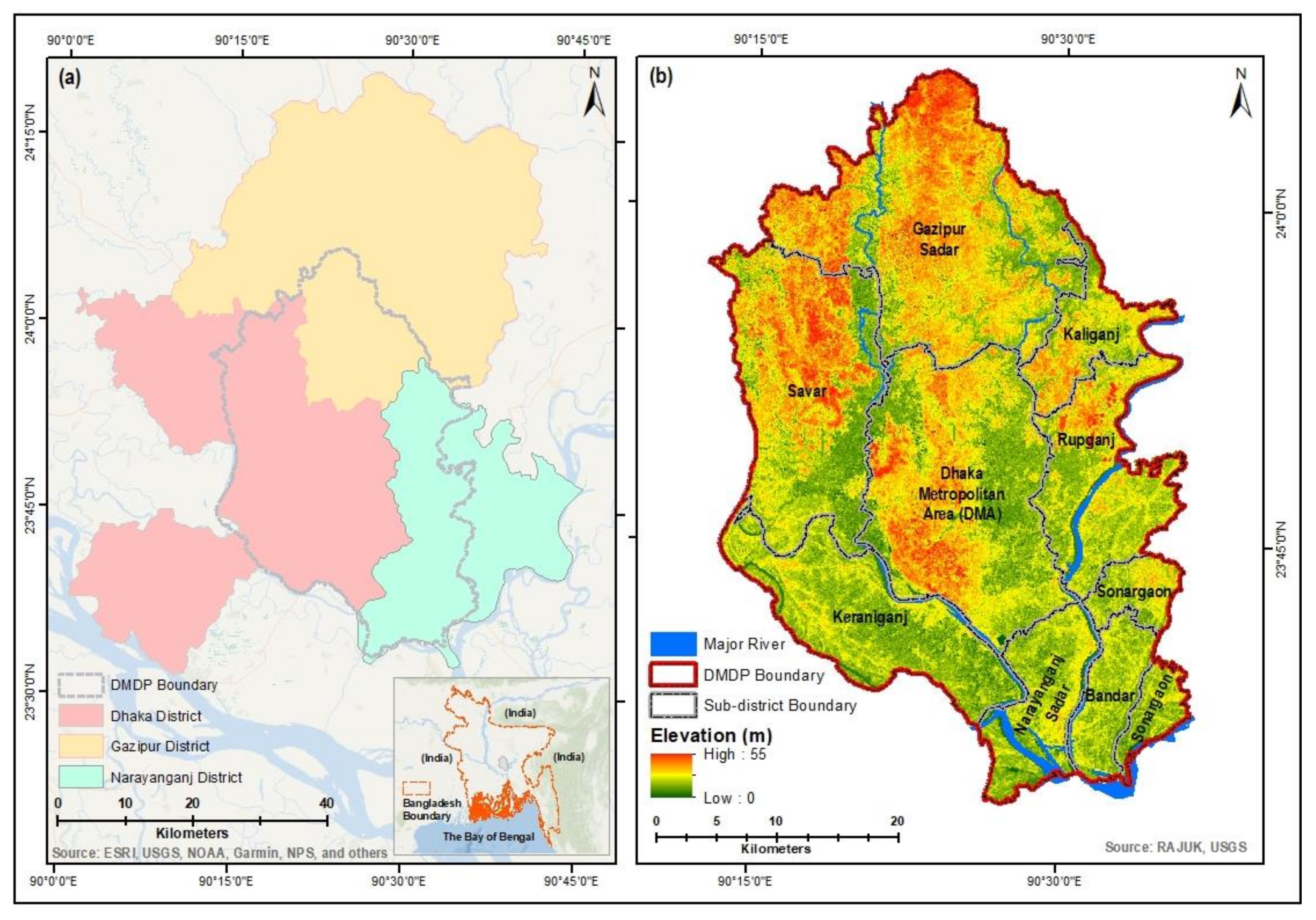
Figure 1. Location of the study area: (a) the Dhaka Metropolitan Development Plan (DMDP) area within the national context; (b) the Dhaka Metropolitan Development Plan (DMDP) area and its corresponding sub-districts’ location.
Remotesensing 12 03938 g001
Figure 2. Methodological steps of this study.
Remotesensing 12 03938 g002
Figure 3. The selection of pseudo light pixels (PLPs) and their adjacent pixels within the frame of a 7 X 7 moving window [48] (p. 404).
Remotesensing 12 03938 g003
Figure 4. (a) The original DMSP-OLS image of 1992 for the DMDP area; (b) self-adjusting model (SEAM)-corrected image of 1992 for the DMDP area; (c) resampled night-time light (NTL) VIIRS image of 2016 for the DMDP area.
Remotesensing 12 03938 g004
Figure 5. The level of urbanization under the microscope of fuzzy linear urban membership function set.
Remotesensing 12 03938 g005
Figure 6. (a) Classified DMDP image from 1989; (b) classified DMDP image from 1999; (c) classified DMDP image from 2009; (d) classified DMDP image from 2019.
Remotesensing 12 03938 g006
Figure 7. (a) % of net changes in bare soil; (b) % of net changes in built-up areas; (c) % of net changes in vegetation; (d) % of net changes in low-land areas.
Remotesensing 12 03938 g007
Figure 8. (a) Peri-urban mapping of 1992; (b) peri-urban mapping of 2016.
Remotesensing 12 03938 g008
Figure 9. (a) Sub-district-wise level of urbanization (LoU) and degree of fuzziness (DoF) statistics for 1992; (b) sub-district-wise level of urbanization (LoU) and degree of fuzziness (DoF) statistics for 2016.
Remotesensing 12 03938 g009
Figure 10. Spatial distribution of ground-truthing points on NTL VIIRS data mapping of 2016 for: (a) predominantly rural areas; (b) peri-urban areas; (c) predominantly urban areas.
Remotesensing 12 03938 g010
Figure 11. Spatial distribution of CRDP’s 2015–2035 proposed land use zones [60].
Remotesensing 12 03938 g011
Figure 12. The level of urbanization (LoU) and degree of fuzziness (DoF) under the CRDP’s 2015–2035 prosed land use zones.
Remotesensing 12 03938 g012
Figure 13. The level of urbanization (LoU) and degree of fuzziness (DoF) for CRDP’s 2015–2035 proposed land use zones: (a) Bandar; (b) Dhaka Metropolitan Area (DMA); (c) Gazipur Sadar; (d) Kaliganj; (e) Keraniganj; (f) Narayanganj Sadar; (g) Rupganj; (h) Savar; and (i) Sonargaon.
Remotesensing 12 03938 g013aRemotesensing 12 03938 g013b
Figure 14. (a) Hot spot analysis of the aggregate population growth rate (APGR) mapping; (b) hot spot analysis of the standard deviation of the average likelihood of poverty (ALP); (c) hot spot analysis of elevation pattern derived from the SRTM global DEM data [43]; (d) Hot spot analysis of the fuzzy linear urban membership function set image of 2016.
Remotesensing 12 03938 g014
Figure 15. Rainfall pattern of the DMDP area.
Remotesensing 12 03938 g015
Figure 16. DMDP’s flood plain area (FPA) (derived from CRDP [60]) superimposed on the VIIRTS NTL data mapping of 2016.
Remotesensing 12 03938 g016
Figure 17. (a) Spatial distribution of 2001 population; (b) spatial distribution of 2016 population; (c) spatial distribution of 2020 population (derived from WorldPop and CIESIN [45]).
Remotesensing 12 03938 g017
Figure 18. (a) Map showing the spatial distribution of predominantly rural (PRURAL), peri-urban (PU), and predominantly urban (PURBAN) areas; (b) table showing percentage distribution in the changes of PRURAL, PU, and PURBAN areas and corresponding changes in the aggregate population growth rate (APGR) between 2001 and 2020; (c) sub-district-wise aggregate population growth rate (APGR) between 2001 and 2020.
Remotesensing 12 03938 g018
Figure 19. (a) Spatial distribution of the average likelihood of poverty (ALP) (i.e., the average probability of living on less than $2.50/day) of 2013 [62]; (b) slum settlement areas (derived from Gruebner et al. [63]) superimposed on the standard deviation (Std. Dev.) of the average likelihood of poverty (ALP) mapping of 2013 [62]; (c) sub-district-wise spatial distribution of the average likelihood of poverty (ALP); (d) sub-district-wise spatial distribution of the standard deviation (Std. Dev.) of the average likelihood of poverty (ALP).
Remotesensing 12 03938 g019
Table 1. Characteristics of Landsat data for the DMDP area [43].
DatePath/RowSensorSatelliteResolution
20 November 1989137/44TMLandsat 530 m
9 March 1989137/44TMLandsat 530 m
1 February 1999137/44TMLandsat 530 m
1 February 1999137/43TMLandsat 530 m
30 January 2010137/44TMLandsat 530 m
28 February 2009137/43TMLandsat 530 m
23 January 2019137/44OLILandsat 830 m
23 January 2019137/43OLILandsat 830 m
Table 2. The radiance values of NTL data between dynamic and persistent built-up areas.
YearPersistent Built-up AreasDynamic Built-up Areas
MinimumMaximumMeanMinimumMaximumMean
1992064.2229.22064.229.0
2016033.3712.82046.46.33
Table 3. Criteria to ground-truth the NTL VIIRS data mapping of 2016.
CategoryCriteria
Predominantly urbanThe ground-truthing point falls in places where the areas maintain a high-density (i.e., apparently, there is no distance between two settlements) continuous built-up development and surrounding areas are built-up.
If the point does not fall within continuous built-up areas, point falls in places from where high-density continuous built-up areas are within 300 m.
Predominantly ruralThe point falls in places where vegetation is more dominant, and a number of scattered rural homesteads are located within 200 m radius
The point falls within the proximity of 300 m radius from the nearby road
Settlements are located proximity to paddy lands, wetlands, or low-lying areas
Peri-urbanLocated within 400 m of low-density continuous built-up development
Located within 50 m from the nearby roads
The point falls in places where vegetation is less dominant (i.e., built-up areas are not shaded by the vegetation) than the presence of built-up areas
Point falls in a location where settlements are dispersed but follows a linear development alongside the road
Table 4. Aerial statistics of classified images for the DMDP area.
Land Cover/Year1989199920092019R2
(Exponential)
Area (Km2)%Area (Km2)%Area (Km2)%Area (Km2)%
Bare soil27418247161521012580.94
Built-up199133292263241790520.97
Vegetation659436364243528320210.92
Water body3834034734230.00
Low land359232771826217252160.83
Total1529100152910015291001529100
Table 5. Aerial statistics of peri-urban growth between 1992 and 2016.
CategoryYear 1992Year 2016% of Changes (1992–2016)
Area (in km2)%LoUDoFArea (in km2)%LoUDoFLoUDoF
Predominantly rural365240.031167110.04133.33%0.00%
Peri-urban715470.30.98874580.40.9433.33%(-)4.08%
Predominantly urban452290.940.07478310.960.122.13%71.43%
Table 6. Confusion matrix of NTL VIIRS data mapping of 2016.
CategoryPredominantly RuralPeri-UrbanPredominantly UrbanTotalProducer’s AccuracyUser’s Accuracy
Predominantly rural30403455.56%88.24%
Peri-Urban24147117289.09%85.47%
Predominantly urban014809498.77%85.11%
Total5416581300
Overall Accuracy86%
Kappa Coefficient0.75
Table 7. Aerial statistics of the proposed land use zone (derived from the CRDP 2015–2035 [60]).
Proposed Land
Use Zoning
Predominantly RuralPeri-UrbanPredominantly UrbanTotal Area
(in km2)
Total %
Area
(in Km2)
%Area
(in Km2)
%Area
(in Km2)
%
Agricultural Zone 86.365.81325.2321.8719.461.31431.0529
Forest Area 4.710.3214.420.970.080.0119.211
Heavy Industrial Zone 0.210.016.600.4423.111.5529.932
Institutional Zone 0.410.0319.811.3338.882.6159.104
Mixed Use Zone58.663.94417.9328.10335.6722.57812.2655
Open Space 1.460.104.720.327.000.4713.181
Transport and Communication 0.940.067.470.5014.770.9923.182
Waterbody 7.400.5056.173.7835.602.3999.167
Table 8. Distribution of population between predominantly rural areas, peri-urban areas, and predominantly urban areas based on NTL VIIRS 2016 data mapping.
CategoryArea
(in km2)
Year 201Year 2016Year 2020
Population%Density
(in Km2)
Population%Density
(in Km2)
Population% Density
(in Km2)
Predominantly rural167148,5831890246,18511474269,27711612
Peri-urban8742,204,1422125223,512,1732040193,999,344214576
Predominantly urban4788,073,6847716,89113,436,2187828,10915,136,3597831,666
Total151910,426,409100686417,194,57610011,32019,404,97910012,775
Publisher’s Note: MDPI stays neutral with regard to jurisdictional claims in published maps and institutional affiliations.