Comparison of ISS–CATS and CALIPSO–CALIOP Characterization of High Clouds in the Tropics

Abstract

Clouds in the tropics have an important role in the energy budget, atmospheric circulation, humidity, and composition of the tropical-to-global upper-troposphere–lower-stratosphere. Due to its non-sun-synchronous orbit, the Cloud–Aerosol Transport System (CATS) onboard the International Space Station (ISS) provided novel information on clouds from space in terms of overpass time in the period of 2015–2017. In this paper, we provide a seasonally resolved comparison of CATS characterization of high clouds (between 13 and 18 km altitude) in the tropics with well-established CALIPSO (Cloud–Aerosol Lidar and Infrared Pathfinder Satellite Observation) data, both in terms of clouds’ occurrence and cloud optical properties (optical depth). Despite the fact that cloud statistics for CATS and CALIOP are generated using intrinsically different local overpass times, the characterization of high clouds occurrence and optical properties in the tropics with the two instruments is very similar. Observations from CATS underestimate clouds occurrence (up to 80%, at 18 km) and overestimate the occurrence of very thick clouds (up to 100% for optically very thick clouds, at 18 km) at higher altitudes. Thus, the description of stratospheric overshoots with CATS and CALIOP might be different. While this study hints at the consistency of CATS and CALIOP clouds characterizaton, the small differences highlighted in this work should be taken into account when using CATS for estimating cloud properties and their variability in the tropics.

1. Introduction

Clouds are a key factor in the Earth’s global radiation budget and then on the Earth’s climate system [1]. Clouds in the tropics are particularly important because of their role in modulating the energy budget, the large-scale atmospheric circulation [2], and the interplay of these components of the Earth system [3]. In the free troposphere, tropical clouds amount and their daily to seasonal cycles are driven largely by convection [4]. Through deep convection, tropical clouds can reach very high altitudes, including stratospheric overshoot, thus impacting on the upper-tropospheric and stratospheric water content, composition, and radiative balance [5]. High clouds in the tropics develop around a limited area of convection centers, in the intertropical convergence zone (ITCZ), which is found at different locations in winter and summer [6], and is rare at other times.

Space LiDARs (Light Detection And Ranging) are important tools towards gaining a better understanding of the vertical distribution of clouds, with high sensitivity to a large spectrum of clouds types (from thin to opaque clouds) and a fine vertical resolution. The Cloud–Aerosol LIdar with Orthogonal Polarization (CALIOP) onboard the Cloud–Aerosol Lidar and Infrared Pathfinder Satellite Observation (CALIPSO) spacecraft has provided a large amount of vertically resolved information on clouds [7] since its launch in 2006. The CALIPSO spacecraft is in a sun-synchronous orbit, with local overpasses at about 01:30 and 13:30 in the tropics. Despite its impressive contribution to cloud science, CALIPSO’s local overpass may not be ideal for assessing high clouds’ properties, processes, and impacts in the tropics—in particular, over land [8]. Over land, convection development, which drives high cloud formation in the tropics, has a peak in the late afternoon [8,9], temporally distant from both CALIPSO overpasses. Thus, CALIOP observations have fundamental limitations in the observation of high clouds in the tropics and, in particular, for the characterization of their diurnal cycle. When constructing longer-terms statistics, this under-representation of the overall high clouds phenomenology may also generate biases in the longer-term characterization of high clouds in the tropics. Since January 2015, the Cloud–Aerosol Transport System (CATS) flies onboard the International Space Station (ISS), in a non-sun-synchronous orbit. With this kind of orbit, different local overpass times are possible. Thus, CATS is expected to provide important complementary and new information on clouds, including high clouds in the tropics. The first studies using CATS have recently been realized, and provided new insights into the diurnally resolved cloud occurrence [10]; the interplay of humidity, convection, and clouds in the tropics [11]; and the occurrence and characteristics of stratospheric overshoot in the tropics [12]. While some first validation of CATS level 2 observations (geophysical parameters and optical properties, like cloud detection or optical depth) has been provided, e.g., with ground-based instruments [10], further validation efforts would be beneficial for gaining more confidence in these first results.

In this paper, we provide a detailed comparison of CATS characterization of high clouds in the tropics with CALIOP data. The comparison with the well-established CALIOP data is chosen to assess the validity of the relatively new CATS data. It is worth mentioning that the present study is not focused on the assessment of the performances of CATS at the diurnal temporal scale, but rather at large spatiotemporal scales, i.e., on the seasonal variability in the whole tropics. The paper is structured as follows: the data and comparison methodology is described in Section 2; comparison results are given in Section 3; conclusion are drawn in Section 4.

2. Data and Methods

2.1. The Cloud–Aerosol Transport System (CATS)

The CATS instrument is a LiDAR system onboard the ISS, orbiting the Earth at about 400 km altitude in non-sun-synchronous geometry. It was in-orbit from January 2015 and ended operations on October 2017 following a failure in the communication subsystem [13]. The ISS orbit limits CATS observations to about 50${}^{\circ }$N–50${}^{\circ }$S (see Figure 1a of [10]). Of the three nominal wavelengths (1064, 532, and 355 nm) only the one at 1064 nm has been operating since March 2015 and has been used in the level 2 algorithms [14]. The analyses of the present paper are based on the cloud detection data of the Vertical Feature Mask level 2 product version 1.0 at 5-km horizontal resolution (day and night) and cloud optical depth (COD). Due to its non-sun-synchronous orbit, CATS observes the same spot on Earth at different times each day. This feature has recently been demonstrated to provide diurnal cycle information on clouds and their properties [10,11,12]. Level 1 CATS data (e.g.m the attenuated total backscatter) have been validated by comparison with CALIOP level 1 data [15]. An initial comparison of Level 2 cloud fraction data from CATS and CALIOP is shown in [10]. The CATS system also provides aerosol data [16] that was not used in the present work.

2.2. The Cloud–Aerosol Lidar with Orthogonal Polarization (CALIOP)

The Cloud–Aerosol LIdar with Orthogonal Polarization (CALIOP) is a LiDAR system onboard the Cloud–Aerosol Lidar and Infrared Pathfinder Satellite Observation (CALIPSO) spacecraft, flying at about 700 km altitude in a sun-synchronous orbit, as part of the A-Train [17]. It has been in orbit since April 2006 and is still in operation. It provides vertical profiles of aerosols and clouds twice a day, at about 01:30 and 13:30 local time. For the present analysis, cloud detection data of the Vertical Feature Mask level 2 version 3.30 at 5 km horizontal resolution, day and night, are used. The two nominal wavelengths, 1064 and 532 nm, are used in the level 2 algorithms.

2.3. Comparison Criteria

The CATS and CALIOP individual profile observations at 5 km horizontal resolution were first aggregated into the different grid-points of the subsequent analyses; statistical samples were then generated. Mean maximum altitude of cloud top and height-resolved high clouds density and optical depth for CATS and CALIOP were compared during the overlapping period 1 January 2015–31 December 2016. The mean maximum altitude of cloud top was calculated as the average, in the selected grid points, of the altitude of the clouds’ tops for the highest cloud layer in each profile forming the grid-point statistics. The high cloud density was defined as the number of observations with cloud tops over a certain altitude (in this paper, from 13 to 18 km) divided by the total number of observations. These comparisons are provided on a seasonal basis (northern hemisphere winter: December–January–February, DJF; and northern hemisphere summer: June–July–August, JJA) on 2.5${}^{\circ }\times {2.5}^{\circ }$ grid. In addition, as this work is not focused on the diurnal cycle of clouds’ occurrence and properties, we did not colocate CATS and CALIOP based on the overpass time, i.e., we used all CATS data in our analyses without screening based on overpass hour (one exception is made in Section 3.2). This is a trade-off between spatial accuracy of our analyses and reasonable in-grid statistics. Both day and night overpasses are considered in the subsequent statistics. Regional comparisons of vertically resolved high cloud density for some of the relevant tropical regions, e.g., defined by Tissier and Legras [18], are also provided.

3. Results

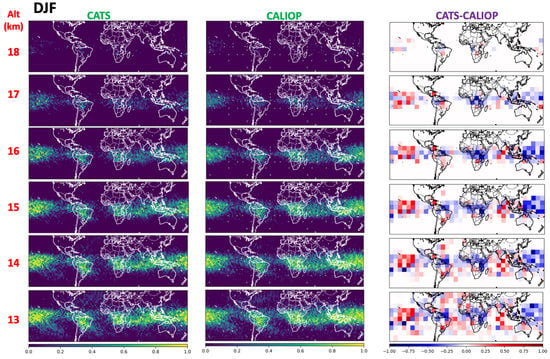
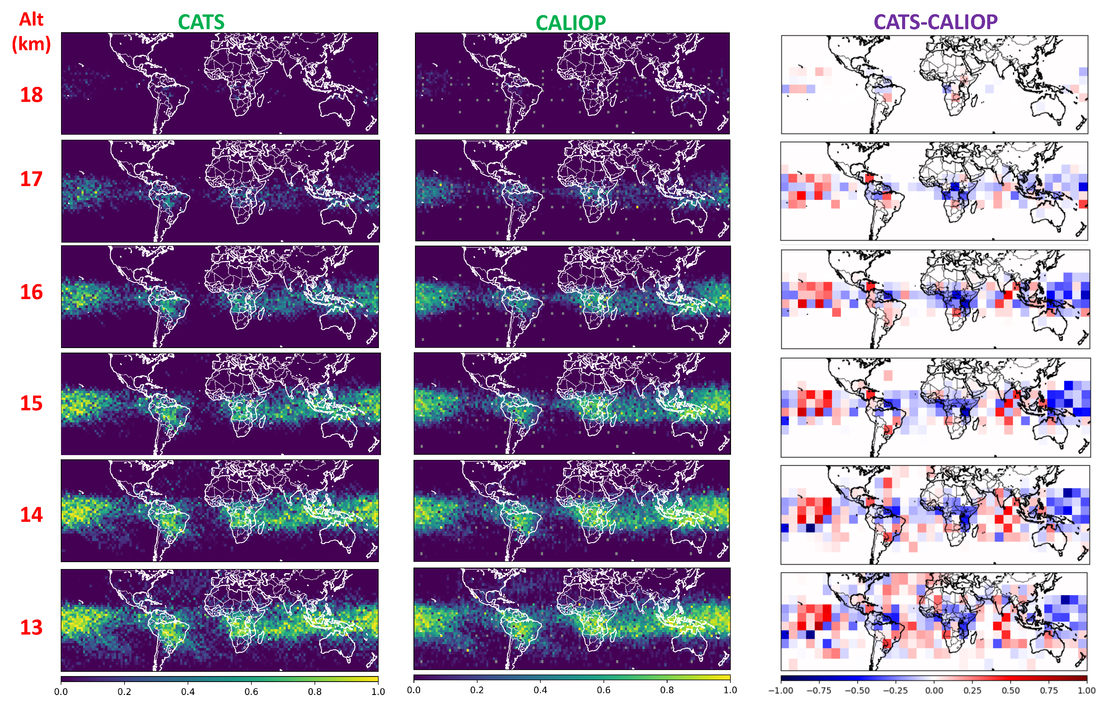
3.1. Spatial Distribution of High Cloud Density

Figure 1a–d show the mean maximum altitude of clouds top from CATS (panels a and b) and CALIOP (panels c and d), for DJF and JJA (panels a and c, and b and d, respectively). The global spatial distributions of mean maximum of the two instruments are consistent. Higher cloud tops are found in DJF over oceans, in particular, in the Tropical Warm Pool. The highest mean cloud tops are found in the tropics, and follow the seasonal variability of the ITCZ. In the ITCZ zones, cloud tops reach mean altitudes of 15 km or larger. To get a more quantitative comparison, in Figure 1e,f, we show histogram of CATS and CALIOP maximum altitude of cloud tops and their differences for DJF (panel e) and JJA (panel f). The histograms of cloud tops are very consistent for the two instruments, with a quasilinear increase up to 15 km and a quick fall for higher altitudes in DJF, and a quasi-bi-modal distribution, with maxima at about 5–6 km and about 14 km in JJA. The difference of CALIOP and CATS mean cloud tops displays a Gaussian-shaped distribution, with a mean value of −0.23 (−0.24) km and standard deviation of 3.04 (2.22) km in DJF (JJA). Thus, CATS displays, on average, a small underestimation of the order of 200 meters of the clouds top height with respect to CALIOP.

Figure 2 and Figure 3 show the global distributions of high cloud density, for CATS and CALIOP and for different altitude thresholds, for DJF (Figure 2) and for JJA (Figure 3), as well as their difference (CATS–CALIOP). Again, the spatial distributions derived with CATS and CALIOP are very consistent with each other. A clear organization of high clouds in the ITCZ is visible both in DJF and in JJA. The ITCZ, and then the maximum density of high clouds, shift from southern to more northern regions, from DJF to JJA. A higher density of high clouds is found in the main seasonal convection centers: Tropical Warm Pool/Maritime Continent, the Indian Ocean, Central Africa, and Equatorial South America in DJF; to mostly India and the Asian Summer Monsoon region and Central America in JJA. High cloud density goes from about 100% (cloud tops exceeding 13 km) to 50–70% (cloud tops exceeding 16 km) to 5–30% (cloud tops exceeding 17–18 km) at the main convection centers, with larger densities during DJF. The highest altitudes are linked to stratospheric overshoot. Using ERA5 (European Centre for Medium-Range Weather Forecasts–ECMWF–ReAnalysis 5) data, Dauhut et al. [12] found typical values for the tropopause altitude of 17.0 to 17.5 km in the main convection center, with slightly higher altitudes during DJF. In our analyses, stratospheric overshoot clouds are found linked to a typical 5–10% density, in the main hotspot convection centers, consistent with the results of Dauhut et al. [12]. It is important to underline that these proportions are only related to specific hotspot areas; when averaging over the whole tropics, less than 1% of all convection systems are expected to penetrate the tropopause [19].

Both regional under- and overestimations of CATS densities, with respect to CALIOP, can be found. In DJF, CATS underestimates high clouds density in the western section of the Warm Pool, while it overestimates it in the eastern section at all altitudes. An overestimation can be seen in the Indian ocean, especially between 13 and 16 km. In JJA, more complicated regional patterns can be seen in the maps of the differences. A slight underestimation is observed in the Asian monsoon area, especially at altitudes between 13 and 15 km. To obtain a more quantitative comparison, in

Table 1. Height-resolved average percent difference (CATS–CALIOP) of high cloud density for DJF and JJA. The differences are averaged in different latitude ranges, following the shift of the intertropical convergence zone (ITCZ). Standard deviations of the percent differences are also reported.

Top Altitude	Percent Difference of Occurrence
	DJF	JJA
13	8.6 ± 59.9%	−4.4 ± 50.7%
14	−10.0 ± 64.5%	−6.6 ± 55.2%
15	−15.2 ± 65.9%	−12.9 ± 60.2%
16	−18.8 ± 69.8%	−13.9 ± 70.0%
17	−36.7 ± 73.2%	−29.8 ± 77.3%
18	−78.9 ± 56.4%	−84.9 ± 42.3%

, we list the average percent difference (CATS–CALIOP) of the high clouds densities of Figure 2 and Figure 3, averaged over the latitude ranges of maximum occurrence of high clouds, i.e., in the seasonal ITCZ. On average, despite a systematic underestimation of the densities, CATS densities are very consistent with CALIOP ones, from top altitudes at 13 km to 17 km. Percent differences for these altitudes range between about −9% (−4%) at 13 km, and −37% (−30%) at 17 km, for JJA (DJF), though with large standard deviations (which reflect the regional inhomogeneities visible in Figure 2 and Figure 3). Larger underestimations of CATS densities, with respect to CALIOP densities, at 18 km, are found (−79% and −85%, for DJF and JJA). Thus, stratospheric overshoot characterizations of CATS and CALIOP may be different.

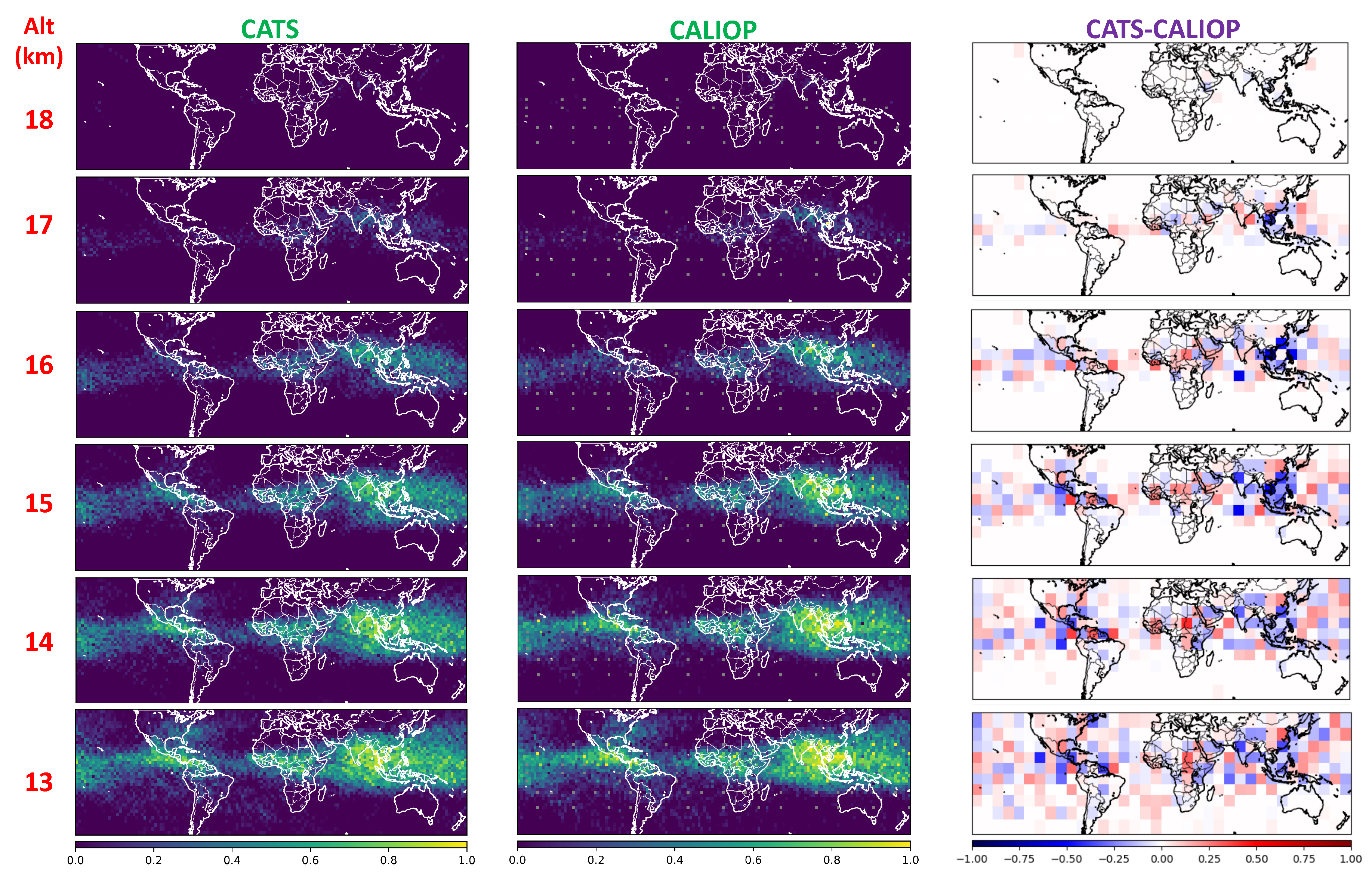
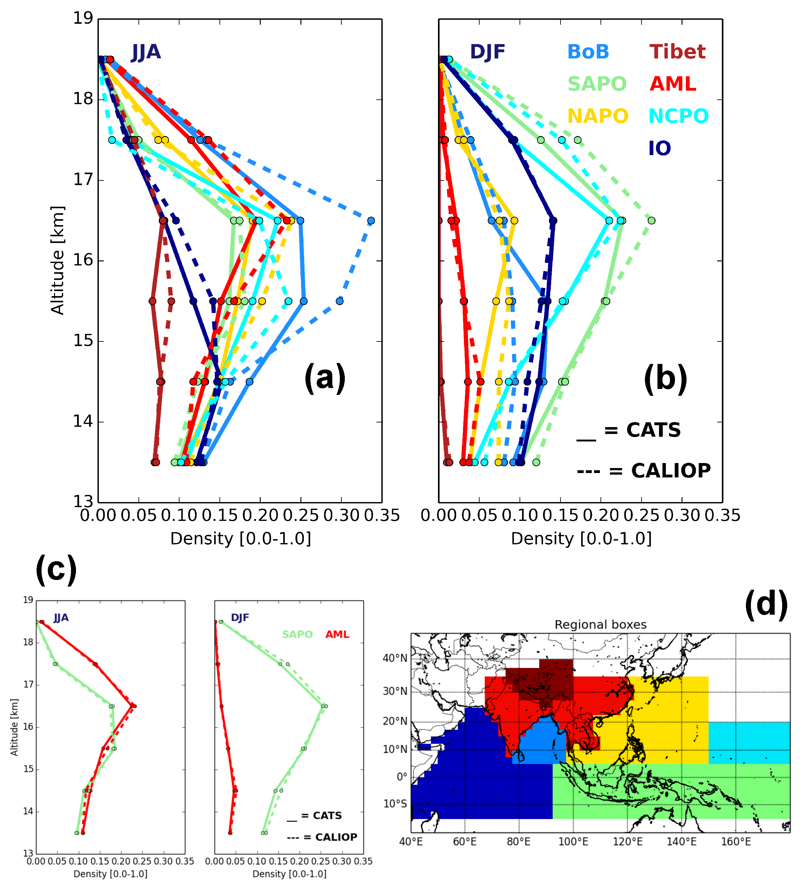
3.2. Vertical Distribution of High Clouds

A particular focus is given here to the core all-year tropical convection area, encompassing the Warm Pool (most active during DJF) and the Asian Summer Monsoon region (most active during JJA) and the height-resolved occurrence of high clouds in this large area. While contributing to high cloud and humidity budget of the upper-troposphere–lower-stratosphere, this area is also a preferential convectively-driven gateway of boundary layer pollution to the tropical tropopause and, through this, the global stratosphere [20]. This has been linked to the occurrence of a seasonal and localized aerosol layer, the Asian Tropopause Aerosol Layer (ATAL) [21]. Following the subdivision of Tissier and Legras [18], we analyze different subregions in this broad area: Indian Ocean (IO), Asian Mainland (AML; corresponding to India and South East Asia, including South East China), the Tibetan Plateau (Tibet), the Bay of Bengal (BoB), the North Asian Pacific Ocean (NAPO), the South Asian Pacific Ocean (SAPO; these two regions including most of the Maritime Continent), and the North Central Pacific Ocean (NCPO; see Figure 4d and the acronyms in the figure caption). The three regions NAPO, SAPO, and NCP aggregate most of the Tropical Warm Pool. Figure 4 show the vertical distribution of cloud density for CATS and CALIOP, in the mentioned subregions, for JJA (panel a) and DJF (panel b). These vertical profiles are linked to the results of Figure 2 and Figure 3. In JJA, a slight systematic underestimation of CATS densities is found at altitudes of peak densities, e.g., 16 km for BoB, AML, and NAPO; and 15–16 km for SAPO. In some cases, the maximum for CATS is shifted in altitude, e.g., 1 km lower for IO and 1 km higher for NCPO. In DJF, a slight CATS density overestimation is found for SAPO and NCPO at peak altitude (16 km), while a slight underestimation is found for BoB at peak altitude (14–15 km). These differences might be linked with the different observation geometries of CATS and CALIOP, and in particular, their different temporal sampling. It is expected that CATS catches, on average, the complete diurnal variability of convection, while this is not expected for CALIOP due to the fixed overpass local time at 01:30 and 13:30, far from the periods of most variable convection and high clouds occurrence [10]. Another possibility is that these differences depend on the different operational wavelengths used by CATS and CALIOP to construct their level 2 clouds’ products. Despite these differences, both space LiDAR identify the same regions and altitude ranges as the most important in terms of high clouds occurrence: BoB (25–35%), AML (20–25%), NAPO (20–25%), and NCPO (20–25%) in JJA; and SAPO (20–25%) and NCPO (20%), in DJF, all at 16 km altitude. To test the impact of different overpass hours, we show the CATS and CALIOP profiles with a temporal colocation of CATS observations (i.e., by considering, in the average profiles, only the CATS observations taken at ±3 h from the day and night CALIOP overpass) for selected regions (SAPO and AML) in Figure 4c. We did not find statistically significant samples for other regions, due to the limited dimensionality of the colocated CATS dataset. From Figure 4c, it is possible to see how the temporal colocation of CATS and CALIOP significantly improves the consistency of these instruments’ observations of high clouds.

3.3. Cloud Optical Depth

Besides the comparison of the occurrence of high clouds, we also compared the optical properties of high clouds in the tropics as seen by CATS and CALIOP. The most straightforward cloud optical property that we discuss in this paper is the cloud optical depth (COD, here at 1064 nm). The COD describes the vertically integrated optical thickness of the cloud. Depending on the altitude, clouds display a large variability of their optical depth and are generally classified as optically thin (typically for COD smaller than 0.3), thick (for COD between 0.3 and 3.0), and very thick/opaque (for COD larger than 3.0). Figure 5 shows normalized histograms of COD for integrated high clouds in the latitude range from 30${}^{\circ }$N to 30${}^{\circ }$S, at altitudes higher than 14 and 18 km, from CATS and CALIOP, for DJF and JJA. In addition, the percent occurrence of COD smaller than 0.3 (thin clouds), within the interval 0.3–3.0 (think clouds), and bigger than 3.0 (very thick clouds) are summarized in Figure 6. To emphasize altitude trends comparisons, these results are shown for three altitudes, 14, 16, and 18 km. Histograms of COD and occurrence of thin, thick, and very thick clouds from CATS and CALIOP data are, in general, consistent. A steeply decreasing distribution of COD occurrence, with increasing COD, is found for both instruments, this decrease being steeper as altitude increases. The proportion of thin clouds increases with the altitude. Typical occurrences of thin, thick, and very thick clouds at 14 km are 74–77% (71–72%), 21–24% (26–27%), and 1.0–1.5% (1.5–2.5%), respectively, in DJF (JJA). Typical occurrences of thin, thick, and very thick clouds at 18 km are 85% (78–79%), 13–14% (19–20%), and 0.5–1.0% (1.0–1.5%), respectively, in DJF (JJA). The more marked differences between the two instruments are that, on average, CALIOP sees slightly more thick clouds, especially in the COD range from 1.0 to 2.5, and CATS sees slightly more very thick clouds. Overall, the larger occurrence of the stratospheric (18 km) very thick clouds in CATS observations reach values as large as 100% during DJF. This can be linked to the larger statistical sample of CATS at peak hours for continental deep convection, due to its non-sun-synchronous orbit. Coupling this result with the results described in Section 3.1, it is apparent as the description of clouds linked to convective overshoots in the stratosphere is different for the two instruments: CATS observes less overshoots but with a larger optical thickness, in particular during DJF.

4. Conclusions

Dominated by convection, tropical clouds can reach very high altitudes, up to the upper-troposphere–lower-stratosphere. Clouds in the tropics have an important role in the global energy budget, atmospheric circulation and hydration and composition of the global stratosphere. Since January 2015, the CATS LiDAR system onboard the International Space Station has provided important information on clouds, including high clouds in the tropics, because of its non-sun-synchronous orbit which allows the vertical sampling of clouds and their properties at different overpass times. This contrasts with the well-established CALIOP LiDAR that sounds the atmosphere at fixed overpass times, far from the convective strength peak of early afternoon, that drives the development of higher tropical clouds. Thus, the CATS observations are to be validated and compared to more established observations, like from CALIOP, so as to gain confidence towards the exploitation of this novel cloud observation capability.

In this paper, we provide a seasonally resolved comparison of CATS characterization of high clouds in the tropics with CALIOP data, both in terms of the clouds occurrence and cloud optical depth. In general, despite the fact that clouds statistics for CATS and CALIOP are generated using intrinsically different local overpass times (all day for CATS, and only at 01:30 and 13:30 local time for CALIOP), the characterization of high clouds occurrence and optical properties (COD) in the tropics with the two instruments is very similar. Both instrument show the same spatial structures and vertically resolved densities of high clouds in the tropics, with a clear organization in the seasonally variable ITCZ around the main seasonal convection centers—Tropical Warm Pool/Maritime Continent, the Indian Ocean, Central Africa and Equatorial South America (DJF), India and the Asian Summer Monsoon region, and Central America (JJA). The mean cloud-top altitude of CATS displays a very small underestimation of the order of 200 meters, with respect to CALIOP. The distribution of CODs are also very consistent for the two instruments, with optically thin clouds largely dominating in the upper-troposphere–lower-stratosphere and their occurrence increasing with the altitude. The most important differences between CATS and CALIOP occur at the highest altitudes, in the lower-stratosphere, where CATS observes up to 80% larger cloud density and up to 100% larger occurrence of optically very thick clouds, with respect to CALIOP. The description of stratospheric overshoots by CATS is different with respect to CALIOP, quite probably due to the different overpasses time; CATS have a larger statistical sample during the peak continental convective activity, which can be linked with less (more aggregated) overshoots with larger optical thickness. Further small differences are found in the vertical partitioning of cloud occurrence in the main convection centers, with small underestimations of CATS occurrences at the altitudes of peak density.

While this study hints at the consistency of CATS and CALIOP clouds characterizaton in the tropics, the small differences highlighted in this work should be taken into account when using CATS for estimating cloud properties in the tropics and their variability.

References

1. Boucher, O.; Randall, D.; Artaxo, P.; Bretherton, C.; Feingold, G.; Forster, P.; Kerminen, V.M.; Kondo, Y.; Liao, H.; Lohmann, U.; et al. Clouds and Aerosols, in Climate Change 2013: The Physical Science Basis. Contribution of Working Group I to the Fifth Assessment Report of the Intergovernmental Panel on Climate Change; Cambridge University Press: Cambridge, UK; New York, NY, USA, 2013; Chapter 7; pp. 571–658. [Google Scholar] [CrossRef]
2. Sherwood, S.C.; Bony, S.; Dufresne, J.L. Spread in model climate sensitivity traced to atmospheric convective mixing. Nature 2014, 505, 37–42. [Google Scholar] [CrossRef] [PubMed]
3. Bony, S.; Stevens, B.; Frierson, D.M.W.; Jakob, C.; Kageyama, M.; Pincus, R.; Shepherd, T.G.; Sherwood, S.C.; Pier Siebesma, A.; Sobel, A.H.; et al. Clouds, circulation and climate sensitivity. Nat. Geosci. 2015, 8, 261–268. [Google Scholar] [CrossRef]
4. Houze, R.A., Jr. Cloud Dynamics; Academic Press: Cambridge, MA, USA, 1993. [Google Scholar]
5. Schoeberl, M.R.; Jensen, E.J.; Pfister, L.; Ueyama, R.; Wang, T.; Selkirk, H.; Avery, M.; Thornberry, T.; Dessler, A.E. Water vapor, clouds, and saturation in the tropical tropopause layer. J. Geophys. Res. 2019, 124, 3984–4003. [Google Scholar] [CrossRef]
6. Pan, L.L.; Munchak, L.A. Relationship of Cloud Top to the Tropopause and Jet Structure from CALIPSO Data. J. Geophys. Res. 2011, 116, D12201. [Google Scholar] [CrossRef]
7. Stephens, G.; Winker, D.; Pelon, J.; Trepte, C.; Vane, D.; Yuhas, C.; L’Ecuyer, T.; Lebsock, M. CloudSat and CALIPSO within the A-Train: Ten Years of Actively Observing the Earth System. Bull. Am. Meteorol. Soc. 2018, 99, 569–581. [Google Scholar] [CrossRef] [Green Version]
8. Matsui, T.; Chern, J.D.; Tao, W.K.; Lang, S.; Satoh, M.; Hashino, T.; Kubota, T. On the Land–Ocean Contrast of Tropical Convection and Microphysics Statistics Derived from TRMM Satellite Signals and Global Storm-Resolving Models. J. Hydrometeorol. 2016, 17, 1425–1445. [Google Scholar] [CrossRef]
9. Emmanuel, K.A. Atmospheric Convection; Oxford University Press: Oxford, UK, 1994. [Google Scholar]
10. Noel, V.; Chepfer, H.; Chiriaco, M.; Yorks, J. The diurnal cycle of cloud profiles over land and ocean between 51 S and 51 N, seen by the CATS spaceborne lidar from the International Space Station. Atmos. Chem. Phys. 2018, 18, 9457–9473. [Google Scholar] [CrossRef] [Green Version]
11. Chepfer, H.; Brogniez, H.; Noel, V. Diurnal variations of cloud and relative humidity profiles across the tropics. Sci. Rep. 2019, 9, 16045. [Google Scholar] [CrossRef] [Green Version]
12. Dauhut, T.; Noel, V.; Dion, I.A. The diurnal cycle of the clouds extending above the tropical tropopause observed by spaceborne lidar. Atmos. Chem. Phys. 2020, 20, 3921–3929. [Google Scholar] [CrossRef] [Green Version]
13. Yorks, J.E.; McGill, M.J.; Palm, S.P.; Hlavka, D.L.; Selmer, P.A.; Nowottnick, E.P.; Vaughan, M.A.; Rodier, S.D.; Hart, W.D. An overview of the CATS level 1 processing algorithms and data products. Geophys. Res. Lett. 2016, 43, 4632–4639. [Google Scholar] [CrossRef] [Green Version]
14. Yorks, J.E.; Palm, S.P.; McGill, M.J.; Hlavka, D.L.; Hart, W.D.; Selmer, P.A.; Nowottnick, E.P. CATS Algorithm Theoretical Basis Document, Level 1 and Level 2 Data Products, release 1.2. In Technical Report; NASA GSFC: Greenbelt, MD, USA, 2016. Available online: https://cats.gsfc.nasa.gov/media/docs/CATS_ATBD.pdf (accessed on 13 February 2018).
15. Pauly, R.M.; Yorks, J.E.; Hlavka, D.L.; McGill, M.J.; Amiridis, V.; Palm, S.P.; Rodier, S.D.; Vaughan, M.A.; Selmer, P.A.; Kupchock, A.W.; et al. Cloud-Aerosol Transport System (CATS) 1064 nm calibration and validation. Atmos. Meas. Tech. 2019, 12, 6241–6258. [Google Scholar] [CrossRef] [Green Version]
16. Proestakis, E.; Amiridis, V.; Marinou, E.; Binietoglou, I.; Ansmann, A.; Wandinger, U.; Hofer, J.; Yorks, J.; Nowottnick, E.; Makhmudov, A.; et al. EARLINET evaluation of the CATS Level 2 aerosol backscatter coefficient product. Atmos. Chem. Phys. 2019, 19, 11743–11764. [Google Scholar] [CrossRef] [Green Version]
17. Winker, D.M.; Pelon, J.; Coakley, J.A.; Ackerman, S.A.; Charlson, R.J.; Colarco, P.R.; Flamant, P.; Fu, Q.; Hoff, R.M.; Kittaka, C.; et al. The CALIPSO Mission. Bull. Am. Meteorol. Soc. 2010, 91, 1211–1230. [Google Scholar] [CrossRef]
18. Tissier, A.S.; Legras, B. Convective sources of trajectories traversing the tropical tropopause layer. Atmos. Chem. Phys. 2016, 16, 3383–3398. [Google Scholar] [CrossRef] [Green Version]
19. Liu, C.; Zipser, E.J. Global distribution of convection penetrating the tropical tropopause. J. Geophys. Res. Atmos. 2005, 110, D23104. [Google Scholar] [CrossRef] [Green Version]
20. Randel, W.; Jensen, E. Physical processes in the tropical tropopause layer and their roles in a changing climate. Nat. Geosci. 2013, 6, 169–176. [Google Scholar] [CrossRef]
21. Vernier, J.P.; Fairlie, T.D.; Natarajan, M.; Wienhold, F.G.; Bian, J.; Martinsson, B.G.; Crumeyrolle, S.; Thomason, L.W.; Bedka, K.M. Increase in upper tropospheric and lower stratospheric aerosol levels and its potential connection with Asian pollution. J. Geophys. Res. Atmos. 2015, 120, 1608–1619. [Google Scholar] [CrossRef] [PubMed] [Green Version]
Figure 1. Mean maximum altitude of cloud top from Cloud–Aerosol Transport System (CATS) (a,b) and Cloud–Aerosol LIdar with Orthogonal Polarization (CALIOP) (c,d), years 2015–2016, day and night overpasses, for December–January–February (DJF) (a,c) and June–July–August (JJA) (b,d). Histogram of CATS and CALIOP maximum altitude of cloud top and their differences (CATS–CALIOP) for DJF (e) and JJA (f).
Remotesensing 12 03946 g001
Figure 2. Global distribution of high clouds density from CATS (left column) and CALIOP (central column), years 2015–2016, day and night overpasses, during DJF. The CATS–CALIOP differences (based on a coarser 10 × 10 grid) are shown as well (right column). The partial cloud covers and the differences are shown for top altitudes from 18 to 13 km (different rows).
Remotesensing 12 03946 g002
Figure 3. Same as Figure 2 but during JJA.
Remotesensing 12 03946 g003
Figure 4. Vertical distribution of cloud density from CATS (solid lines) and CALIOP (dashed lines), in the altitude range 13–18 km for JJA (a) and DJF (b). Same as (a,b) but with CATS data temporally colocated with CALIOP overpasses, for selected regions (c). The seven subregions indicated in (d) are individuated with corresponding colors. A description of acronyms follows. IO: Indian Ocean, AML: Asian MainLand, Tibet: Tibetan Plateau, BoB: Bay of Bengal, NAPO: North Asian Pacific Ocean, SAPO: South Asian Pacific Ocean, NCPO: North Central Pacific Ocean.
Remotesensing 12 03946 g004
Figure 5. Normalized histograms of cloud optical depth (COD) for integrated high clouds at altitudes higher than 14 and 18 km from CATS (red bars) and CALIOP (blue bars) for DJF (left column) and JJA (right column). Note the logarithmic vertical scale.
Remotesensing 12 03946 g005
Figure 6. Percent occurrence of COD smaller than 0.3 (thin clouds, blue lines, left vertical scale), within the interval 0.3–3.0 (thick clouds, red lines, left vertical scale) (a) and bigger than 3.0 (very thick clouds, green lines, right vertical scale) (b), from CATS (solid lines) and CALIOP (dotted lines) for DJF (dark-colored lines) and JJA (light-colored lines).
Remotesensing 12 03946 g006