Article

Comparing Forest Structural Attributes Derived from UAV-Based Point Clouds with Conventional Forest Inventories in the Dry Chaco

1
Earth and Life Institute, George Lemaître Center for Earth and Climate Research, Université Catholique de Louvain, Place Pasteur, 1348 Louvain-la-Neuve, Belgium
2
Division of Geography and Tourism, Department of Earth and Environmental Sciences, KU Leuven, 3001 Leuven, Belgium
3
Institute of Regional Ecology, CONICET, National University of Tucumán, CC34, CP 4107 Yerba Buena, Tucumán T4107, Argentina
*
Author to whom correspondence should be addressed.
Remote Sens. 2020, 12(23), 4005; https://doi.org/10.3390/rs12234005
Submission received: 2 October 2020 / Revised: 25 November 2020 / Accepted: 30 November 2020 / Published: 7 December 2020
(This article belongs to the Section Forest Remote Sensing)

Abstract

:
Anthropogenic activity leading to forest structural and functional changes needs specific ecological indicators and monitoring techniques. Since decades, forest structure, composition, biomass, and functioning have been studied with ground-based forest inventories. Nowadays, satellites survey the earth, producing imagery at different spatial and temporal resolutions. However, measuring the ecological state of large extensions of forest is still challenging. To reconstruct the three-dimensional forest structure, the structure from motion (SfM) algorithm was applied to imagery taken by an unmanned aerial vehicle (UAV). Structural indicators from UAV-SfM products are then compared to forest inventory indicators of 64 circular plots of 1000 m2 in a subtropical dry forest. Our data indicate that the UAV-SfM indicators provide a valuable alternative for ground-based forest inventory’ indicators of the upper canopy structure. Based on the correlation between ground-based measures and UAV-SfM derived indicators, we can state that the UAV-SfM technique provides reliable estimates of the mean and maximum height of the upper canopy. The performance of UAV-SfM techniques to characterize the undergrowth forest structure is low, as UAV-SfM indicators derived from the point cloud in the lower forest strata are not suited to provide correct estimates of the vegetation density in the lower strata. Besides structural information, UAV-SfM derived indicators, such as canopy cover, can provide relevant ecological information as the indicators are related to structural, functional, and/or compositional aspects, such as biomass or compositional dominance. Although UAV-SfM techniques cannot replace the wealth of data collected during ground-based forest inventories, its strength lies in the three-dimensional (3D) monitoring of the tree canopy at cm-scale resolution, and the versatility of the technique to provide multi-temporal datasets of the horizontal and vertical forest structure.

1. Introduction

Forests cover about 25% of Earth’s terrestrial surface. In 2013, only 24% of the remaining forests are part of intact forest landscapes with no detectable human pressure [1]. Intact forests play a key role in climate change mitigation, regulation of local climate regimes and hydrological services, biodiversity conservation, and human health [2,3]. Published case studies have shown that intact forests store 10% to 55% more carbon than logged, degraded or planted forests in ecologically comparable locations [2]. Mapping the existing variability in forest characteristics, including the physical structure, species composition and functional organization of forest ecosystems can provide insights in the anthropogenic pressures on forests and natural disturbance regimes, and provide foundations for environmental impact mitigation [4,5].
In recent years, the use of ultra-high resolution aerial images captured by digital cameras installed on unmanned aerial vehicles (UAVs) has been growing steadily for forest monitoring [6,7]. The combination of consumer grade technologies—UAVs and digital image processing—created new opportunities for forest monitoring. Computer vision techniques such as structure from motion, paired with multi-view stereo algorithms (commonly abbreviated as SfM), allows one to extract three-dimensional (3D) information from a set of overlapping images using iterative bundle adjustment procedures [8]. The UAV-SfM products cover areas of 0.1 to 100 km2, with a spatial resolution of 100 to 100,000 points per m2 [9]. Clapuyt et al. [10] showed that the precision of measurements is in the order of centimeters for identical replications.
The SfM-based surveys from unmanned aerial vehicles have several advantages compared to other active or passive sensors [6,9,11]: lightweight UAVs have the flexibility of vertical or short take-off and landing, they are easy to deploy to collect information in difficult-to-access terrain, and can carry relatively low-cost, off-the-shelf visible range or multispectral cameras for SfM-based surveys. Within the context of forest inventories, Dandois and Ellis [12] were one of the first who demonstrated the performance of UAV SfM-based methods to produce 3D high-resolution forest canopy models, and to derive metrics of the physical structure of forest ecosystems. Feasibility studies of UAV-SfM techniques for forest inventories by e.g., Puliti et al. [13] and Tuominen et al. [14] in boreal forests have shown accuracies (in terms of RMSE%) of 3.5% for dominant height, 15 to 24% for basal area, and 39% for stem density. More recent studies in the Amazonian forest by Messinger et al. [15], mangrove forests in Malaysia [16] and conifer-broadleaved in Japan [17] have shown similar performances. As stated in the review of SfM applications in forestry by Iglhaut et al. [6], previous studies mainly dealt with mature to nearly mature closed forests, and much less so with open forests or fragmented forests. A significant part of open and fragmented forest is located in tropical dry forests [18].
Given the increasing human pressure on dry tropical forests, it is essential to monitor the evolution of their forest structure, function, and species composition. The structure refers to the spacing and height of the various components of the forest ecosystem. The percent tree cover, trunk height, vertical canopy complexity, and understory density are all structural attributes affecting animal abundance and diversity [19,20,21]. The ecosystem functions refer to the different biological, geochemical, and physical processes that take place within the forest ecosystem, such as the production of organic matter. The species composition is the identity and variety of ecosystem components and is characterized by species richness and abundance [22]. These attributes are often interdependent, and attributes from one group may also act as surrogates for another group [22].
It is crucial to define relevant ecological indicators that allow one to characterize these forest attributes. In this study, we aim to identify the structural indicators derived from UAV-SfM point clouds and canopy height models that can properly characterize structural, functional, and compositional forest attributes and can be defined as ecological indicators. First, we assessed the performance of UAV-SfM based methods by comparing forest structural attributes derived from UAV-based point clouds and ground-based forest inventories. We then analyzed which structural indicators are meaningful ecological proxies of forest structure, ecosystem function, and species composition. Through the analyses, we tested whether accounting for both the vertical and horizontal complexity of the forest stratum allows to better discriminate landscape-scale forest composition. Our study is conducted in the Dry Chaco forest where forest inventory data is available from sixty-four forest plots covering each 1000 m2. The novelty of this research lies in (i) the validation of UAV-SfM forest structural attributes based on forest inventory indicators of 64 circular plots of 1000 m2, and (ii) the publication of—to our knowledge—one of the first applications of UAV-SfM techniques to the Dry Chaco forest ecosystem. Furthermore, this study analyses multiple ecological attributes by accounting for forest structure, composition, and function.

2. Methods

2.1. Study Area

The Gran Chaco is the second largest natural biome in South America and extends over ca. 1.3 million km2. The intact landscape of the region was mostly characterized by patches of hard wood forests and natural pastures [23]. The Dry Chaco (Figure 1A), the eastern part of the Gran Chaco covers an area of 0.8 million km2 and it extends over Argentina, Paraguay, and Bolivia. Its vegetation is adapted to arid conditions with broadleaf and deciduous or semi-deciduous species [24]. Cabrera [25] discerned three vertical forest strata. The first consists the canopy stratum dominated by Schinopsis lorentzii (quebracho colorado santiagueño), Bulnesia sarmientoi (Palo Santo), and Aspidosperma quebracho-blanco (quebracho blanco). The second arboreal or sub-canopy stratum comprises Ziziphus mistol, Geoffroea decorticans, Caesalpinia paraguariensis, Tabebuia nodosa, Prosopis alba, P. nigra, P. kuntzei, and others. The third shrub stratum can be very dense and is typically composed of Acacia spp. Schinus spp., Salta triflora, Capparis spp., Celtis spp., and others.
Anthropogenic activities modified the vegetation cover and composition of the Dry Chaco over the last two centuries [23]. The presence of high-value hardwood species boosted large-scale wood exploitation and processing industry for tannin extraction. Since 1880, landscape modification increased because of railway expansion in the Argentinean Chaco. During the last two decades, the tannin production is declining while the wood exploitation continues resulting in forest degradation [26]. Besides selective logging of high-value timber, exploitation for firewood and charcoal remains important in areas hosting people under extreme poverty [27]. The “puestos” system that is characterized by traditional settlements and extensive cattle ranching also plays a role in forest degradation and shrub encroachment [28]. The anthropogenic land use likely changed the Chaco landscape from a mosaic of woodlands, savannas and shrublands to a landscape vegetation pattern dominated by secondary forests and dense thickets of shrubs [29,30].

2.2. Forest Inventory Data

Field data on forest structure, function, and composition is available from forest inventory plots that were monitored by the Instituto de Ecología Regional of the University of Tucumán [24,32]. In the Dry Chaco, fifty forest vegetation clusters were surveyed on a regular basis, starting in 2007, and revisited in 2012 and 2017–2019. Of the fifty clusters, we selected sixteen clusters as to cover the existing gradient in forest degradation state. Each cluster contains four circular forest inventory plots of 1000 m2 (Figure 2), resulting in 16 × 4, i.e., 64 forest inventory plots. With a Garmin 12XL and eTrex Legend H GPS, we determined the absolute location of the center of each plot with a precision of 2 to 3 m. The position of individual trees within the plot was then measured in a relative coordinate system, measuring the azimuths and distances to the plot center. For the field inventory, the circular plots are divided in two concentric circles, with an inner and outer circle of respectively 500 and 1000 m2 (Figure 2). In the inner circle, all trees with a diameter at breast height (DBH) greater than 0.1 m are recorded, while only trees with a DBH greater than 0.2 m are documented in the outer circle. During the forest inventory, the team documented the tree species, and measured for each individual tree (n = 2022) the DBH with diameter tape (m). The tree height (m) was determined in 24 of the 64 inventory plots using trigonometric methods using a clinometer and laser distance meter. In 16 plots, tree height was estimated using visual estimations techniques. The basal area (m2) was derived from the DBH. The aboveground biomass (Mg·ha−1) of tree species was estimated from the DBH measurements and published data on wood specific gravity [33] using the allometric equations presented in Table 1 [34,35].
Table 1 presents the plot-level indicators on forest structure, species composition and function. The forest structure is characterized by its vertical and horizontal complexity. Forest inventories provide data on the structural complexity at the plot-level: the tree height (and its variation), the diameter at breast height (and its variation) and the spatial tree density. For the analysis of the vertical structure of the forest, we set the lower height limits for the three forest strata, the canopy, sub-canopy, and shrubby stratum, at respectively 6 m, 4 m, and 0.5 m. The delimitation of the canopy layer (above 6 m) is the same used by Powell et al. [36] and somewhat different from work by de Casenave et al. [37] and Prado [38], and is here set at the lower height limit of the crown of the canopy. To select this threshold, we evaluated different canopy height values and defined the height for which all the crowns of the larger trees were included in the upper canopy height. To characterize the plot-level species composition, we classified the plots in four groups according to their dominant tree species. This classification is based on the review of the Chaco flora by Prado [38]. Category 1 contains plots that have a dominance of tree species that are characteristic for old-growth stage forests, such as Aspidosperma quebracho-blanco, Schinopsis lorentzii, and Bulnesia sarmientoi. Category 2 and 3 contain plots that have species from the first arboreal stratum as dominant species: Zizyphus mistol for Category 2, and Caesalpinia paraguariensis and Tabebuia nodosa for Category 3. Category 4 regroups the plots that have a dominance of colonizer or pioneer species, like Prosopis nigra, characteristic for degraded or logged forests [37,39].

2.3. UAV Data Acquisition and SfM Image Processing

High-resolution aerial images of the forest canopy were taken with a consumer-grade quadcopter, the Phantom 4 Pro. It is equipped with the standard DJI camera-gimbal system, having a 1-inch 20 megapixel CMOS sensor with a 8.8 mm/24 mm (35 mm format equivalent) FOV lens with f/2.8–f/11 auto focus at 1 m–∞. The UAV data were acquired in the dry southern hemisphere winter, i.e., July to September 2017 and 2018. The flight missions were planned using the Altizure app (Everest Innovation Technology, 2018) appropriate for 3D oblique photogrammetry. For each forest inventory cluster including four plots of 1000 m2, the UAV survey covered an area of 300 m by 300 m centered on the forest plot. The surveys were realized with the team that participated in the forest inventories, to ensure that the forest plots were correctly represented in the UAV surveys. The ground surface was surveyed twice, using both a nadir-oriented and a 30°-tilted camera. The inclusion of oblique images in the SfM algorithm decreases systematic errors in topographic reconstruction and captures better complex 3-D structures as shown by Clapuyt et al. [10]. The frontal and side overlap were set to 80%, following Dandois et al. [40] who suggested 80% as an optimal overlap for UAV-SfM reconstructions of forest structure. The UAV platform flew at a constant height of 80 to 120 m above the take-off point, leading to a ground sample distance between 21.8 and 45.3 mm. Table 2 resumes the camera, flight, and imaging parameters of the flights.
The 3D point clouds were generated from overlapping optical images with the structure from motion algorithm (SfM) in the AgiSoft Photoscan ® software (Professional Edition, version 1.2.4, St. Petersburg, Russia). The SfM process typically starts detecting thousands of features in each image and matches features between images [41,42]. During this step of photo aligning, the software estimates the camera positions, refines the camera calibration, and creates a sparse point cloud. Then, the program calculates depth information from the estimated camera positions to create a single dense point cloud. In this study, we used on average 180 (min. 160, max. 217) aerial photographs per plot, leading to an average point cloud density of 324 points per m2. The 3D point clouds were georeferenced directly using position information from the onboard GPS/GLONASS receiver. This approach ensured a mean absolute horizontal accuracy of 2.6 m. Given horizontal errors of c. 2 to 3 m on the location of 3D point clouds and forest inventory plots, the two datasets were manually co-registered by identifying pairs of corresponding survey trees and aerial detected trees using the cm-scale resolution aerial imagery.
Using the elevation of the 1st percentile of the height data as threshold, we classified the data of the 3D point cloud as ground and non-ground (or vegetation) data points. We tested this procedure on roads and vegetation openings using the orthophotos and verified that it performed well in the very flat topography that characterizes the Dry Chaco. Additionally, the observation and interpretation of the point cloud histograms validated this methodological step. The digital terrain model was generated from the ground class of the 3D point cloud, and the digital surface model from the vegetation point class. The canopy height model (CHM) was then obtained by subtracting the terrain model from the surface model. For further analysis, the 3D vegetation point cloud and canopy height model were clipped using the limits of the forest inventory plots. Data processing was done in R version 3.6.0 using rgdal, sp, rmapshaper, stats, spatialeco, rgeos, and raster packages for percentiles calculation, buffering, clipping, and data processing.

2.4. Image Processing and Variable Extraction

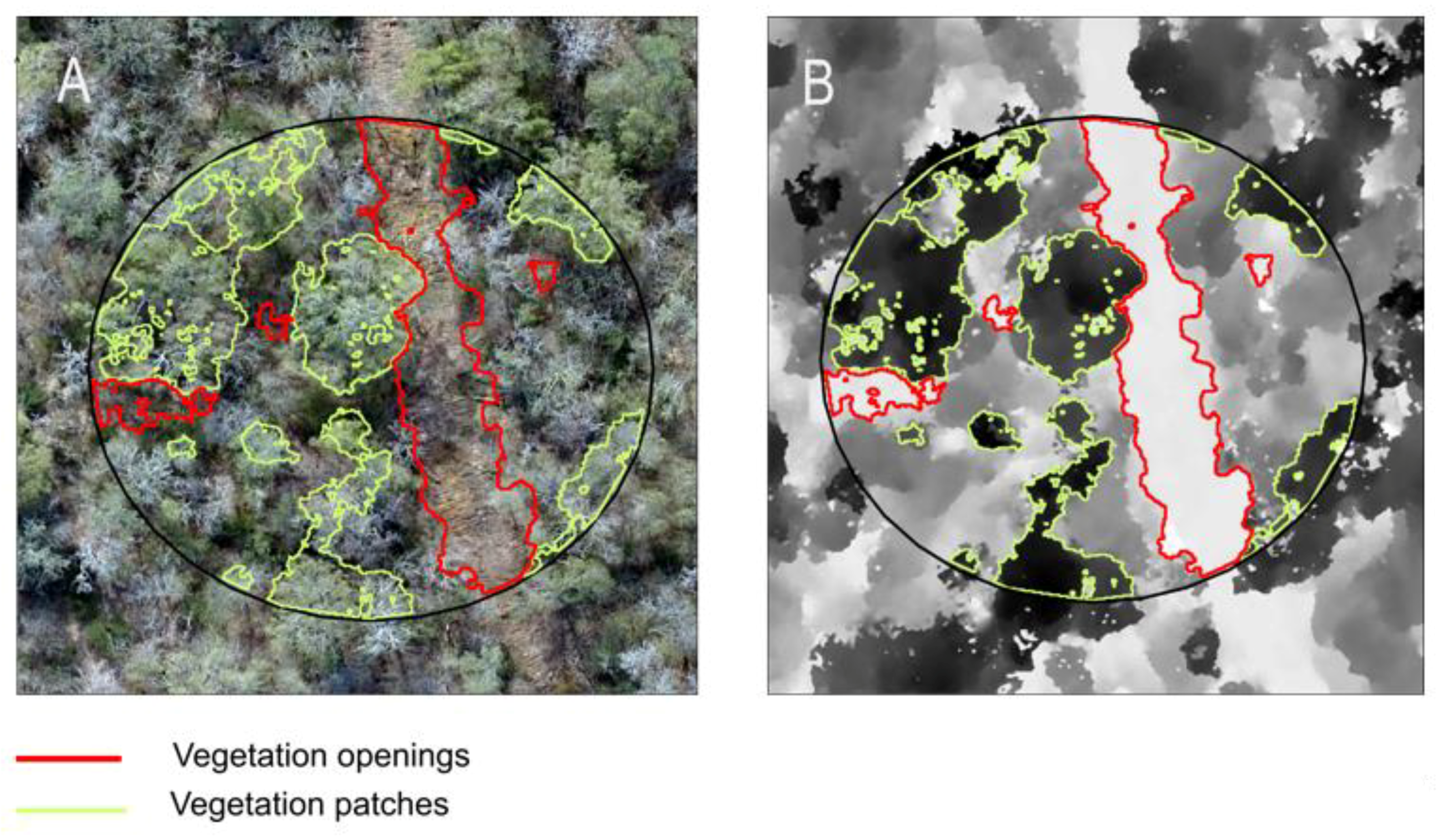
The canopy height model (CHM) served as a basis to extract indicators of forest structure, notably of the spatial distribution of large trees and vegetation openings (Table 3 and Figure 3). Segmentation algorithms as the ones used by e.g., Guerra-Hernández et al., Lim et al. or St-Onge et al. [43,44,45] for automatic detection of individual tree crowns were for some plots overpredicting and for others underpredicting in the Dry Chaco. Therefore, we defined vegetation patches as the areas of the canopy height model where the elevation of the vegetation is above six meters based on image filtering as in Zellweger et al. [46]. Using an R script, pixels with an elevation lower than six meters were masked out, and the remaining clusters of pixels were converted to polygons with the RasterToPolygons function followed by the Disaggregate function from the raster package (Table 3). Hereby, we assume that the clusters correspond to individual tree crowns of the largest trees. The maximum canopy height within the polygon was taken as the height of the individual tree. Similarly, we applied image filtering techniques to extract patches of vegetation openings (Table 3). They were here defined as areas with vegetation smaller than 0.5 m and covering minimum 10 m2. At the plot level, the percentage of the plot with vegetation openings (%) was extracted as an indicator of the horizontal forest structure. Table 4 resumes the four indicators that were derived at the plot level: the mean height of trees taller than 6 m (m), the maximum height of the tallest canopy patch (m), the canopy cover (%), and vegetation openings (%).
In addition to the four CHM-derived indicators of the horizontal forest structure, the information on the vertical forest complexity was derived from the 3D point cloud. This includes information on the structure of the sub-canopy tree branches and foliage, shrubs and grasses that can be present in the understory vegetation. The first two indices are based on the percentiles of the height distribution of the point cloud (Table 4). The 99th percentile of the height distribution is assumed to correspond to the maximum canopy height. The vertical distribution index is adapted from Goetz [20]. It typically shows low values in areas with a dense canopy and a sparse understory, and high values in areas with a more evenly vertical distribution. The third index, the vertical complexity, is a measure of the vertical distribution of points within the three-dimensional point cloud, and is assumed to reflect forest structural properties and stages of stand development [19,47]. The vertical complexity index is based on Pielou’s evenness index [48], and it indicates to what extent the points are evenly distributed throughout the vertical column. The evenness value is at maximum (i.e., 1) when the different height bins have an equal number of points. When the distribution of points within the vertical column becomes more uneven, the evenness value decreases. Following van Ewijk et al. [47], a low value corresponds to an initiation stage with dominance of colonizer or pioneer species; a mid-range value to a dominance of arboreal stratum; and a high value to old growth stage forest with an even distribution of points within the cloud.
In addition, two density-based indicators are derived from the point cloud metrics. They are based on the relative point cloud density, a metric that is widely used in LiDAR data processing for characterization of forest understory structure [49]. By using the overall relative point density (ORD) of the UAV-SfM point cloud, we assume that the likelihood of having the vegetation recorded in a specific height stratum of the SfM point cloud increases as the vegetation density in that height stratum increases. Here, we derived the ORD for two forest strata: the 0.5 to 4 m height stratum corresponding to the shrub vegetation, and the 4 to 6 m height stratum of sub-canopy vegetation.

2.5. Data Analysis

To characterize the forest structure, composition, and function in the study site, we first performed a quantitative analysis of the ground-based variables and the UAV-SfM based structural indicators. Table 5 and Table 6 provide summary statistics for all ground-based and UAV-SfM based variables, and Figure 4 and Figure 5 show the frequency distributions. We then assessed the performance of the UAV-SfM based indicators by comparing the forest structural attributes derived from the canopy height models and point clouds with the forest indicators from ground-based forest inventories. We tested whether UAV-SfM based indicators of forest horizontal and vertical complexity are reliable for the characterization of forest structure. While height data was available for only 40 plots (656 trees), data on diameter at breast height and species composition was collected in all 64 plots (2021 trees). The UAV-SfM indicators on canopy height, and vegetation density per stratum were compared with their equivalent ground-based measures through scatterplots and Spearman correlation analyses (Figure 6 and Figure 7). Ordinary least squares regression techniques were applied to the height indicators to determine the relation between the UAV-SfM indicators and the ground-based measures, and the RMSE was calculated. The UAV-SfM based forest indicators that do not have an equivalent in ground-based inventories, such as canopy cover and vegetation openings, were compared against plot-level information on overall tree density and tree density per DBH class (<0.2 m, between 0.2 and 0.3 m, >0.3 m). Boxplots of the UAV-SfM structural indicators categorized according to their dominant species were plotted with a kernel density distribution. The chi-squared (X2) statistic from the Kruskal-Wallis test and the pair-wise Wilcoxon test were used to detect significant differences between groups. Finally, scatterplots and Spearman correlation analyses were used to visualize and analyze the correlation between biomass and the UAV-SfM structural indicators.

3. Results

3.1. Forest Structure, Composition, and Function Based on Ground-Based Measures

For the 40 plots of 1000 m2 for which tree height data are available, the mean height of the upper canopy ranges between 7.5 and 16.0 m, with a mean and standard deviation of 10.3 ± 1.8 m. The distribution is slightly left-skewed (Figure 4A), and similar to the distribution of values of the height of the tallest tree. The tallest tree is on average 15.3 ± 2.7 m, with a minimum of 10.2 and a maximum a 21.7 m. The number of trees above 6 m is slightly left-skewed, ranges from 70 to 300 trees per hectare, with a mean of 153.0 ± 60.7 trees·ha−1 (Figure 4C). The percentage of trees in the shrubby and the sub-canopy strata varies strongly between plots, with values ranging between 0.0 and 64.1% for the shrubby and between 6.2 to 55.0% for the sub-canopy. The average and standard deviation for the 0.5 to 4 m and 4 to 6 m height strata are respectively 10.4 ± 16.5% and 21.2 ± 14.9%.
The density of trees on the plots varies between 100 and 560 trees per hectare, with an average of 231.1 ± 94.4 trees·ha−1. With regard to forest structure, we observe that more than half of the trees (i.e., 107 ± 86.8 trees·ha−1) have a DBH < 0.20 m, followed by slightly less than 30% having a DBH between 0.2 and 0.3 m, and less than 20% having a DBH > 0.3 m. However, the number of trees < 0.2 m had a high range and variance (i.e., respectively 480 and 86.8 tree·ha−1). Additionally, there are strong differences between plots in the above ground biomass, with values ranging between 12.8 and 62.9 Mg·ha−1 with an average of 30 ± 11.3 Mg·ha−1. About 50% of the 64 plots have the iconic tree species of the dry Chaco forest as dominant species, i.e., Aspidosperma quebracho-blanco, Schinopsis lorentzii, or Bulnesia sarmientoi. Forty percent of the plots have a dominance of sub-canopy species and the remaining 10% have a dominance of pioneer species.

3.2. Horizontal and Vertical Forest Complexity Based on UAV-SfM Data

For the 64 plots, nine indicators were extracted from the point cloud and canopy height model (Table 3 and Table 4). The mean height of the vegetation patches varies between 6.1 and 11.2 m, with an average of 8.1 ± 1.2 m. As shown in Figure 5A, its distribution is left-skewed. Compared to the mean height of the vegetation patches, the height of the tallest vegetation patch shows a wider spread with values between 6.9 and 17.6 m, and average value of 12.8 ± 2.4 m. The canopy cover shows a normal distribution (Figure 5C), varying between 2.8 to 56.6%, and average of 25.6 ± 10.8%. In the 64 plots, the vegetation openings are generally small and of minor extent, with more than 84% of the plots having values below 15%.
From the 3D point cloud, one indicator on forest height was extracted, i.e., the height of the 99th percentile of the vegetation. This indicator has a similar range as the height of the tallest vegetation patch with average value of 11.3 ± 2.2 m. The vertical distribution of the vegetation is strongly right-skewed (Figure 5F) with values ranging from 0.4 to 0.9, and with an average of 0.7 ± 0.1. The vertical complexity has an average value of 0.7 ± 0.1 and ranges from 0.5 to 0.8. None of the plots has a vertical complexity index above 0.8 (Table 6). The relative density of the point cloud is higher in the 0.5 to 4 m stratum compared to the 4 to 6 m stratum, with an average of 50.2 ± 15.2% compared to 15.9 ± 9.5%.

3.3. Performance of UAV-SfM Based Indicators on Forest Structure

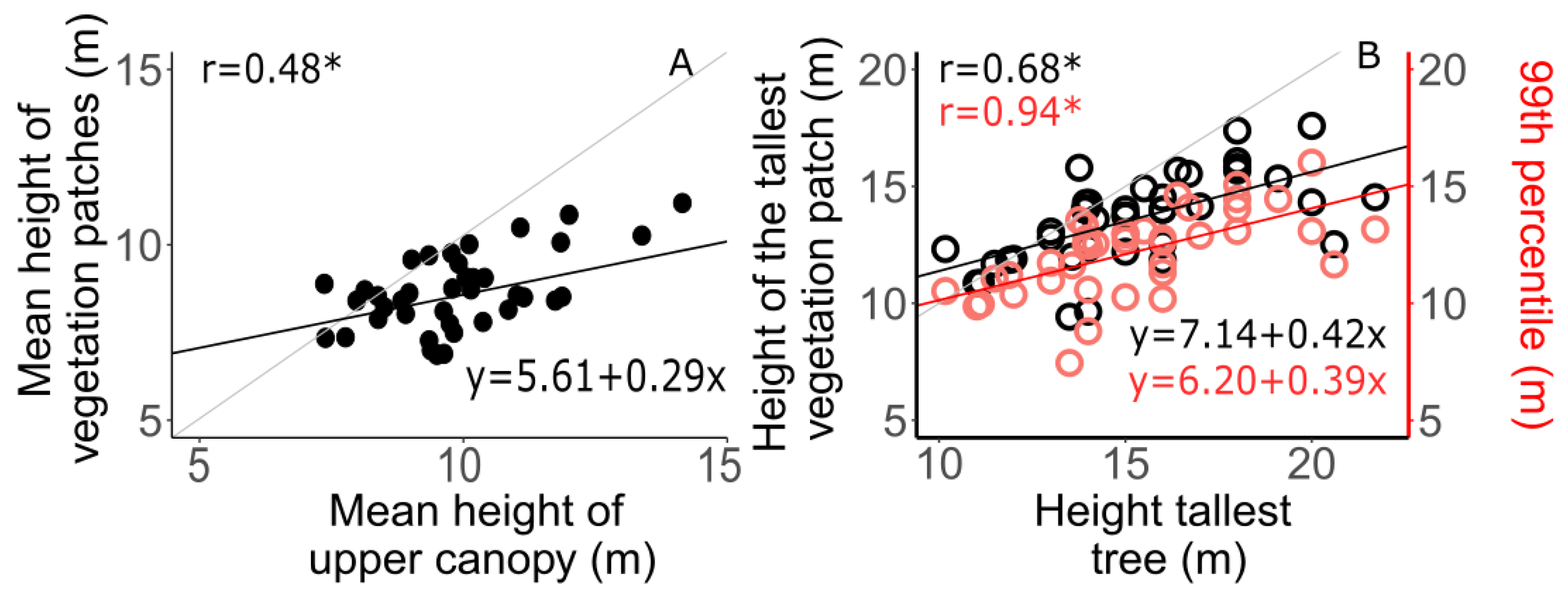
The UAV-SfM based information on canopy height is derived from the canopy height model and point cloud. The maximum height of the tallest canopy patch and the 99th percentile of canopy height distribution are indicators of the maximum tree height, while the mean height of the vegetation patches is an indicator of the mean height of the upper canopy stratum (>6 m). Figure 6A compares the mean height of vegetation patches with mean height of trees above 6 m. Figure 6B compares the two maximum height indicators with the ground-based measures of the tallest tree height (Table 1 and Table 3). Significant correlations between the UAV-SfM based on indicators of canopy height and the ground-based measures were founded for the mean height of tree crown patches and upper canopy (r = 0.48, p < 0.01; RMSE = 1.56 m); the height of the tallest vegetation patch and height of the tallest tree (r = 0.68, p < 0.01; RMSE = 2.14 m) and the 99th height percentile and tallest tree height (r = 0.94, p < 0.01; RMSE = 2.15 m). Interestingly, the majority of data points fall below the 1:1 line, indicating that the estimates of canopy height from UAV-SfM data are systematically lower than the ground-based height measurements (Figure 6).
The vegetation density per stratum estimated from the UAV-SfM point cloud was contrasted with ground-based data on the percentage of trees in the plots that belong to the same stratum. The analyses focused on two strata: the sub-canopy (4–6 m height) and the shrubby (0.5–4 m height) stratum. Figure 7A,C illustrate the poor correlation between the UAV-SfM based relative point density (ORD) data and the ground-based indicators for the 0.5 to 4 m (r = 0.09) and 4 to 6 m stratum (r = −0.08). Instead, the ORD data show a better correlation with ground-based measures of tree DBH (Figure 7B,D). The relative point density in the 0.5–4 m stratum shows a positive correlation with the percentage of trees with DBH < 0.2 m (r = 0.45, p < 0.01). In the sub-canopy stratum, the correlation is not significant.
The UAV-SfM derived information on canopy cover and vegetation openings cannot directly be compared to field-based indicators on forest structure. As both of them are indicators of the horizontal forest structure, the information was validated by comparison with plot-level data on overall tree density per plot (Figure 8), tree density per DBH class (Figure 8 and Figure 9), and number of trees taller than 6 m (Figure 9). The vegetation openings show no correlation with the overall tree density per plots (Figure 8A), and none with the number of trees with DBH above 0.2 m (Figure 8C,D). There is a negative correlation between vegetation openings and the number of trees with DBH below 0.2 m (r = −0.31, p-value = 0.01): plots with large vegetation openings (>10%) have a lower number of small trees (with DBH < 0.2 m, Figure 8B). In contrast to the vegetation openings, canopy cover is significantly related to the density of large trees, with significant positive correlation with the number of trees taller than 6 m (Figure 9A, r = 0.40, p-value < 0.01) and the number of large trees with DBH > 0.3 m (Figure 9B, r = 0.57, p-value < 0.01).

3.4. Relevance of UAV-SfM Based Indicators for Forest Composition and Function

Structure, composition, and function are interdependent attributes of the forest. We assess whether the UAV-SfM based structural indicators are indicative of forest composition described based on the plot-level species composition (Figure 10). In particular, group 4 with dominance of pioneer species shows the largest differences with the other three forest composition groups. Regarding forest height, Figure 10A shows that the forest composition group 4 has a mean height of vegetation patches of 6.5 ± 1.2 m (significantly lower than 8.0 ± 1.1 and 8.5 ± 1.2 m for composition groups 1 and 2). Its height of the tallest vegetation patch is 9.1 ± 1.7m, significantly lower than group 2 with a height of 14.0 ± 2.2 m (Figure 10B). For the 99th percentile (Figure 10E), significant differences are observed between forest composition group 4, and groups 1, 2 and 3. For the overall relative density, differences are significant between groups 1 and 2 compared to 3 and 4 (Figure 10I). The vertical distribution allows to further distinguish between the different stages of forest growth, with median values of 0.8 ± 0.1 and 0.7 ± 0.1 for categories 1 and 2 and significantly lower values of 0.6 ± 0.1 and of 0.5 ± 0.1 for category 3 and 4 (Figure 10F).
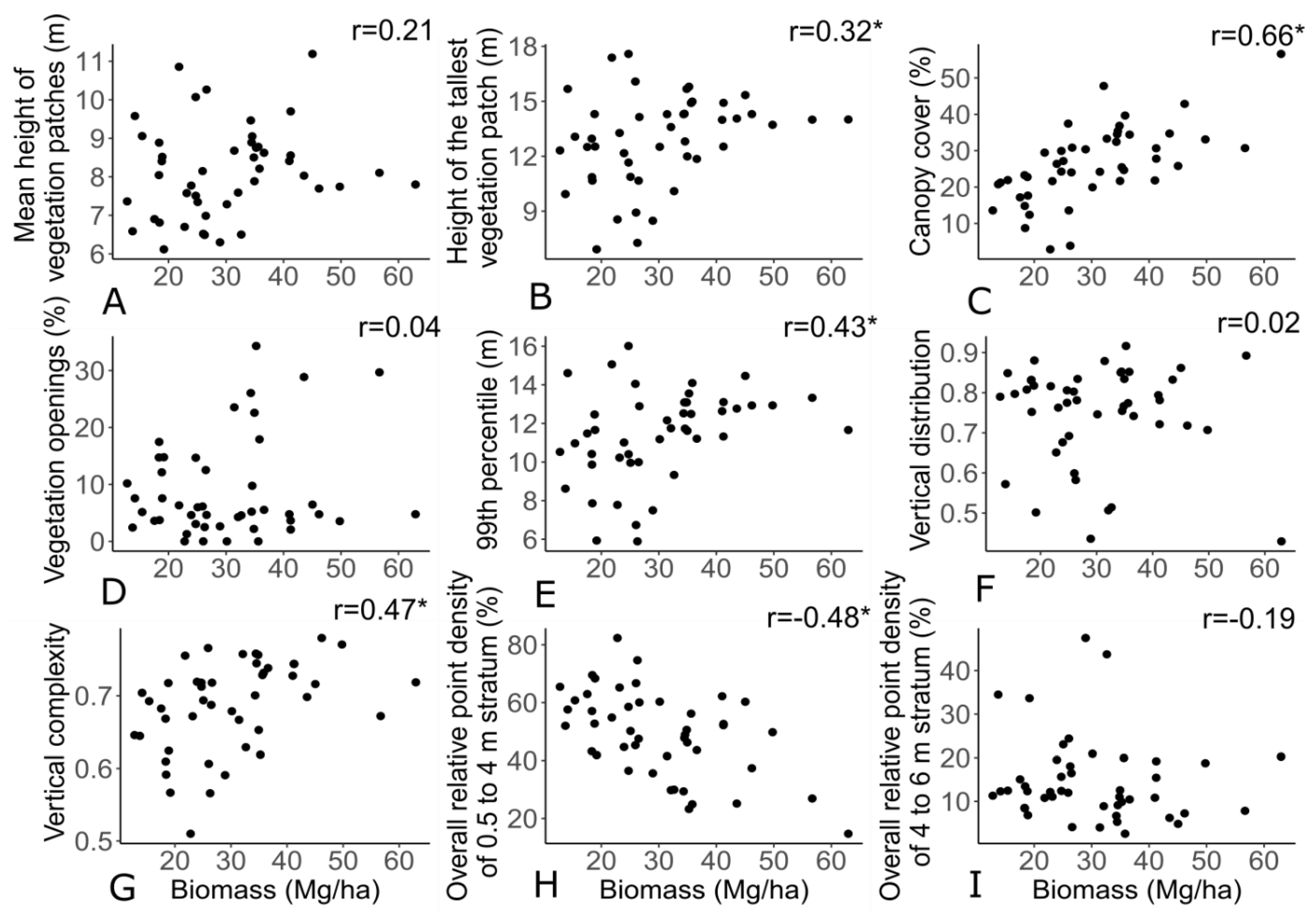
To measure the interdependence of UAV-based structural indicators with forest functional attributes, we analyzed the association between structural indicators and the above ground biomass (Figure 11). The canopy cover (Figure 11C) and the vertical complexity (Figure 11G) are positively related to the above ground biomass (with resp. r = 0.66, p <0.05, and r = 0.47, p < 0.05). Additionally, the height of the tallest vegetation patch (Figure 11B) and the 99th percentile (Figure 11E) are positively related to the above ground biomass (with resp. r = 0.32, p < 0.05 and r = 0.43, p < 0.05) despite that the mean height of the vegetation patches are uncorrelated to it. Finally, the density of the point cloud in the 0.5 to 4 m stratum is negatively related to above ground biomass (r = −0.48, p < 0.01).

4. Discussion

4.1. Forest Structural Indicators as Ecological Indicators

Ecological indicators are used to assess the condition of the environment or to monitor trends in environmental conditions over time [50]. They quantify the magnitude of stress, the degree of exposure to stress, and/or the degree of ecological response to exposure [50]. The three primary attributes of ecosystems—composition, structure, and function—determine and constitute the biodiversity of an area and are interdependent [51]. These attributes are nested at different levels of ecosystem organization—the landscape, community, and population level—and environmental stresses will be expressed distinctively at different levels of organization [51].
Forest inventories are able to evaluate community-level forest attributes and use trees as the basic units. For this reason, many UAV SfM-based surveys derive forest structure metrics at the individual tree level using tree crown detection algorithms. Although these algorithms perform well in conifer forests [45,52], they are known to have lower performance in deciduous forests [52]. In the Dry Chaco forest, the preliminary tests of crown detection algorithms showed poor performance. Therefore, this study was performed on vegetation patches that are considered to be individual trees. These patches of individual trees were compared with structural indicators from forest inventories. Even though UAV-SfM techniques only provide direct observations of forest structures, the UAV-SfM derived indicators can be linked with compositional and functional indicators from the forest inventory as forest composition, structure and function are interdependent. The forest composition was studied by classification of forest plots by their dominant tree species, as indicator species are widely used to monitor or assess environmental condition in ecology and other environmental sciences [51]. The presence and/or abundance of indicator species give us information about the state of the forest. The forest function was monitored based on the biomass. Forest biomass is one of the indirect indicators of age, density, successional stage, and productivity which can influence habitat selection and biodiversity [53]. Additionally, it is a valuable indicator for assessing the capacity of the forest to stock carbon for climate change mitigation.

4.2. Horizontal Forest Complexity

4.2.1. Indicators of the Upper Canopy Structure

Tree height is an important ecological trait: the competition for sunlight determines which trees flourish and it influences shades in streams and changes in understory vegetation. The species of the upper strata of the Dry Chaco are characterized by a very slow growth rate [54]. In fact, Bulnesia sarmientoi has an annual growth of 1 mm [32] and Schinopsis lorentzii of 1.6 mm [55]. Because of slow growth rates, estimated at 1 to 3 mm per year, disturbances in the upper canopy structure only recover over large periods of time [54].
Figure 6 allows us to assess the performance of the UAV-SfM based methods to derive plot-level information on upper canopy height. The mean height of the vegetation patches was estimated with a low RMSE of 1.56 m, and the height of the tallest vegetation patch with RMSE of 2.14 m. These results are slightly better as those obtained by Dandois and Ellis [56] and Dandois et al. [40] who predicted the mean height of the five tallest trees of the plots from UAV-SfM data with an overall RMSE of 3.6 to 3.76 m. Puliti et al. [13] revealed lower RMSE values (0.7–1.5 m) on forest height indicators derived from UAV-SfM imagery in conifer-dominated boreal forests.
The canopy height estimates from UAV-SfM data are systematically lower than the field-based measures of tree height (Figure 6). The difference between the two becomes larger with increasing tree height. This is coherent with previous findings by Wang et al. [57] who observed that the height of the upper canopy is often overestimated in field campaigns. Possible sources of measurement error have been widely discussed in the literature. The study by da Silva et al. [58] indicated that the accuracy of field-measured tree heights decreases with increasing tree height and often leads to systematic overestimation of the height of the highest trees. Furthermore, the measure may be sensitive to stand complexity, crown classes, and species [57]. Field measurements of tree heights also require a clear view of the tree base and treetop, which is not always feasible in forests with dense understory such as the thorny Dry Chaco forests.
Overall, we observe that the maximum height of the forest canopy is better represented by the UAV-SfM data than the mean height. Importantly, the UAV-SfM based indicator of canopy height that was directly derived from the 3D point cloud—the 99th percentile—shows the highest correlation (r = 0.94) with the field-based measures of forest height (Figure 6B). This shows that 3D point cloud data allows a better representation of the forest height structure than data derived from vegetation patches. When delineating vegetation patches, the estimates of the canopy height likely increase due to edge effects [59]. In field inventories, the trees are treated as being inside the plots only if 50% of the rooted base of the tree is contained within the plot. This is different in the UAV-SfM based data, as all the tree crown patches located in the plots are considered to be part of the forest plot. The maximum height is less affected than the mean height indicator by the edge effects, as the maximum height is derived for one single tree crown patch that has a lower probability to be located on the edge of the plot.
Canopy height indicators from UAV-SfM data appear to be valuable ecological indicators as they allow us to distinguish the four forest composition groups (Figure 10). The maximum height indicators show significant differences between the three groups with species characteristic for old-growth stage and first arboreal stratum and the composition group 4 with pioneer species. As expected, the 99th percentile height of group 4 is significantly lower than the height of the other three groups. Interestingly, the maximum height indicators are good predictors of the above ground biomass (Figure 11B,E) while the mean height of the canopy patches is not statistically correlated to the above ground biomass. We hypothesize that this is related to the fact that the tallest trees have large diameters and are the ones comprising the largest amount of the above ground biomass [60]. Thereby, they are the ones with the highest influence on the above ground biomass, changes in the mean height of the other trees do not influence statistically the above ground biomass.

4.2.2. Canopy Cover

Canopy cover has been defined as one of the principal parameters describing forests [61,62]. The canopy cover is usually not included in conventional forest inventories, despite the existence of specific ground-based methods [63]. In the Dry Chaco, no ground measurements are available for canopy cover. Baumann et al. [31] established tree cover gradients in the Dry Chaco by modeling Google Earth Engine high resolution imagery with regional remote sensing data.
The UAV-SfM based indicator of canopy cover was compared to the number of trees in the upper canopy (higher than 6 m) and to the number of large trees (DBH > 0.3 m). The canopy cover shows a strong positive correlation (r = 0.57) with the number of large trees. The scatterplot of the canopy cover against the number of trees above 6 m shows more spread in the data and lower correlation coefficient (r = 0.40). We attribute this to the fact that the threshold of DBH of 0.3 m allows to discriminate the largest trees in the forest that are characterized by the largest canopies and have the largest influence on the overall canopy cover. It confirms earlier findings of McElhinny et al. [22] that the number of trees exceeding a threshold diameter is an important forest structural attribute.
The UAV-SfM based canopy cover is the best predictor for aboveground biomass (Figure 11C), and strong indicator of forest functional attributes in the Dry Chaco. This result is coherent with the strong correlation that we observed between canopy cover and the number of large trees (DBH > 0.3 m) as trees with the largest canopy are able to stock a large amount of biomass.

4.2.3. Vegetation Openings

Similar to canopy cover, indicators of vegetation openings are poorly validated in the literature, and rarely quantified by ground-based measurements. Tools such as hemispherical photographs or terrestrial laser scanners are not well suited for this purpose [64]. Here, we assessed vegetation openings from the canopy height model. We observed that the number of thin trees (DBH < 0.2 m) is systematically lower for plots having more than 10% of the area with vegetation openings. The negative correlation is significant but there is a lot of spread in the data (Figure 8).
This indicator is not able to distinguish compositional categories (Figure 10) and has no relation with biomass (Figure 11). Morales-Barquero et al. [65] discusses that the use of this ecological indicator might be compromised by rapid filling of vegetation openings by in-growth of the canopies of the adjacent trees or by recovery of a lower stature vegetation through natural regeneration. This rapid recolonization of the open spaces by shrubby or pioneer species might explain the low potential of this indicator to predict functional or compositional states.

4.3. Vertical Forest Complexity

4.3.1. Sub-Canopy and Shrub Stratum

Understory vegetation plays a critical role in forest ecosystems and it is often the most species rich and diverse portion of a forest [49,66]. However, the assessment of this understory vegetation is regularly excluded from forest inventories and UAV-SfM based research. In our study, shrubs are under-represented in the field inventory because of the error-prone and time-consuming task of inventorying shrub species in the Dry Chaco forest. On the other hand, the representation of the lower forest strata in the UAV-SfM point cloud may be affected by the presence of dense upper canopy. A study by Wallace et al. [67] showed the low ability of SfM-UAV data to represent the forest understory in SfM point clouds when the upper canopy is dense. Even though, we tested the relevance of UAV-SfM indicators to characterize the sub-canopy and shrub stratum.
As expected, the overall relative density of the different stratum cannot be considered as valuable indicators for the sub-canopy and shrub stratum characterization. Even if there is significant correlation with the percentage of trees with DBH below 0.2 m (Figure 7), this indicator is influenced itself with the upper canopy density. Even though, the overall relative density in the 4 to 6 m stratum indicator distinguishes compositional groups (Figure 10) and identifies category 4 that is dominated by trees like Prosopis nigra with relatively high ORD in the 4 to 6 m stratum.

4.3.2. Vertical Distribution and Vertical Complexity

Vertical distribution and vertical complexity are similar indicators as they describe the overall structure of the point cloud. Both indicators were found to be of great utility, as predictors of bird species richness [20] and habitat breeding species [19]. Here, we affirm that vertical distribution and complexity are good predictors of forest functional groups and allow one to identify composition group 4 with pioneer species (Figure 10). Additionally, the forest complexity is a good predictor of the above ground biomass (Figure 11). Then, this type of indicators may be of great utility for monitoring forest, successional stages, or detecting natural or anthropogenic disturbances.

5. Conclusions

By comparing the UAV-SfM forest indicators with ground-based structural indicators, we demonstrated the suitability of UAV-SfM techniques for assessing forest structure using datasets from the dry Chaco. In addition, we studied the relation between UAV-SfM based indicators and ground-based functional and compositional indicators. Indicators on the upper canopy height derived from UAV-SfM data are valuable alternatives for conventional forest inventories, as they have similar or even better accuracy. Particularly, the 99th percentile of the point cloud is a good predictor of the height of the tallest tree (r = 0.94), and performs better than other UAV-SfM structural indicators such as the height of the tallest vegetation patch or the mean height of the vegetation patch. All height indicators are significantly related to the forest compositional groups. Additionally, the height of the tallest tree is a reasonable predictor (r = 0.43) of the above ground biomass. Because of the low growing rates in the dry Chaco, the tree height indictors are valuable indicators of the degree of forest disturbances.
Canopy cover is widely used in the definition of forests and degradation. The UAV-SfM derived indicator of canopy cover is highly correlated with the number of large trees, an important forest structural attribute, and is the best predictor for above ground biomass (r = 0.66). This confirms the relevance of canopy cover as a highly valuable ecological indicator. In contrast, the UAV-SfM derived indicator on vegetation openings is not significantly related to the vegetation density in the lower strata, neither with any of the tested functional or composition attributes of the forests. It is likely that the UAV-SfM indicators are not able to capture accurately the understory structure in dense forests because of the presence of the upper canopy.
The results for the Dry Chaco forests show that UAV-SfM techniques allow one to measure forest structural characteristics and complement labor-intensive inventory techniques. The UAV-SfM methods require an initial investment in capital and human capacity that is lower compared to alternative high-resolution remote sensing techniques, such as terrestrial or airborne laser scanning. The methodology presented in this paper could be used to assess the forest ecological states in different parts of the Dry Chaco as well as in other dry ecosystems. For applications on steep topographies or in landscapes with closed forest canopy the empirical relations that we established for the Dry Chaco will require recalibration. Moreover, the presented UAV-SfM procedure for forest ecological indicators could be a very useful tool for documenting forest status in the framework of applications for conservation funds.

Author Contributions

V.V. conceived the project in collaboration with B.G., I.G. and A.V.R. B.G. performed the UAV flights in collaboration with I.G., D.L. and V.V. B.G. performed the UAV-SfM analyses at UCLouvain. I.G. and D.L. collected the field data in the forest inventory plots. All authors contributed to elaboration of the project and analyses, as well as the writing of the paper. All authors have read and agreed to the published version of the manuscript.

Funding

This work was supported by the Stereo III Research Programme for Earth Observation of the Belgian Federal Science Policy office (Belspo) [ReForCha project, grant number SR/00/338]; the Fondo Nacional de Ciencia y Técnología (FONCyT) [grant PICTO 2011 N° 0098]; B.G. Field work was granted by Fonds Wetenschappelijk Onderzoek (FWO) [grant number 58601]; D.L. Field work was granted by Rufford foundation.

Acknowledgments

We acknowledge the Argentinean administration of the National Parks and their forest rangers (Parque Nacional Copo and Reserva Natural Formosa). We would also like to thank François Clapuyt for the UAV training sessions and Teresa de Marzo, Pedro Fernandez and Philipp Gaertner for field work collaboration.

Conflicts of Interest

The authors declare no conflict of interest.

References

  1. Potapov, P.; Hansen, M.C.; Laestadius, L.; Turubanova, S.; Yaroshenko, A.; Thies, C.; Smith, W.; Zhuravleva, I.; Komarova, A.; Minnemeyer, S.; et al. The Last Frontiers of Wilderness: Tracking Loss of Intact Forest Landscapes from 2000 to 2013. Sci. Adv. 2017, 3, e1600821. [Google Scholar] [CrossRef] [PubMed] [Green Version]
  2. Watson, J.E.M.; Evans, T.; Venter, O.; Williams, B.; Tulloch, A.; Stewart, C.; Thompson, I.; Ray, J.C.; Murray, K.; Salazar, A.; et al. The Exceptional Value of Intact Forest Ecosystems. Nat. Ecol. Evol. 2018, 2, 599–610. [Google Scholar] [CrossRef] [PubMed]
  3. Balthazar, V.; Vanacker, V.; Molina, A.; Lambin, E.F. Impacts of Forest Cover Change on Ecosystem Services in High Andean Mountains. Ecol. Indic. 2015, 48, 63–75. [Google Scholar] [CrossRef]
  4. Venter, O.; Sanderson, E.W.; Magrach, A.; Allan, J.R.; Beher, J.; Jones, K.R.; Possingham, H.P.; Laurance, W.F.; Wood, P.; Fekete, B.M.; et al. Sixteen Years of Change in the Global Terrestrial Human Footprint and Implications for Biodiversity Conservation. Nat. Commun. 2016, 7, 1–11. [Google Scholar] [CrossRef] [PubMed] [Green Version]
  5. Piperno, D.R.; McMichael, C.N.H.; Bush, M.B. Finding Forest Management in Prehistoric Amazonia. Anthropocene 2019, 26, 100211. [Google Scholar] [CrossRef]
  6. Iglhaut, J.; Cabo, C.; Puliti, S.; Piermattei, L.; O’Connor, J.; Rosette, J. Structure from Motion Photogrammetry in Forestry: A Review. Curr. For. Rep. 2019, 5, 155–168. [Google Scholar] [CrossRef] [Green Version]
  7. Apostol, B.; Petrila, M.; Lorenţ, A.; Ciceu, A.; Gancz, V.; Badea, O. Species Discrimination and Individual Tree Detection for Predicting Main Dendrometric Characteristics in Mixed Temperate Forests by Use of Airborne Laser Scanning and Ultra-High-Resolution Imagery. Sci. Total Environ. 2020, 698, 134074. [Google Scholar] [CrossRef]
  8. Westoby, M.J.; Brasington, J.; Glasser, N.F.; Hambrey, M.J.; Reynolds, J.M. “Structure-from-Motion” Photogrammetry: A Low-Cost, Effective Tool for Geoscience Applications. Geomorphology 2012, 179, 300–314. [Google Scholar] [CrossRef] [Green Version]
  9. Passalacqua, P.; Belmont, P.; Staley, D.M.; Simley, J.D.; Arrowsmith, J.R.; Bode, C.A.; Crosby, C.; DeLong, S.B.; Glenn, N.F.; Kelly, S.A.; et al. Analyzing High Resolution Topography for Advancing the Understanding of Mass and Energy Transfer through Landscapes: A Review. Earth-Sci. Rev. 2015, 148, 174–193. [Google Scholar] [CrossRef] [Green Version]
  10. Clapuyt, F.; Vanacker, V.; Van Oost, K. Reproducibility of UAV-Based Earth Topography Reconstructions Based on Structure-from-Motion Algorithms. Geomorphology 2016, 260, 4–15. [Google Scholar] [CrossRef]
  11. Clapuyt, F.; Vanacker, V.; Schlunegger, F.; Van Oost, K. Unravelling Earth Flow Dynamics with 3-D Time Series Derived from UAV-SfM Models. Earth Surf. Dyn. 2017, 5, 791–806. [Google Scholar] [CrossRef] [Green Version]
  12. Dandois, J.P.; Ellis, E.C. High Spatial Resolution Three-Dimensional Mapping of Vegetation Spectral Dynamics Using Computer Vision. Remote Sens. Environ. 2013, 136, 259–276. [Google Scholar] [CrossRef] [Green Version]
  13. Puliti, S.; Ørka, H.O.; Gobakken, T.; Næsset, E. Inventory of Small Forest Areas Using an Unmanned Aerial System. Remote Sens. 2015, 7, 9632–9654. [Google Scholar] [CrossRef] [Green Version]
  14. Tuominen, S.; Balazs, A.; Saari, H.; Pölönen, I.; Sarkeala, J.; Viitala, R. Unmanned Aerial System Imagery and Photogrammetric Canopy Height Data in Area-Based Estimation of Forest Variables. Silva Fenn. 2015, 49, 1–19. [Google Scholar] [CrossRef] [Green Version]
  15. Messinger, M.; Asner, G.P.; Silman, M. Rapid Assessments of Amazon Forest Structure and Biomass Using Small Unmanned Aerial Systems. Remote Sens. 2016, 8, 615. [Google Scholar] [CrossRef] [Green Version]
  16. Otero, V.; Van De Kerchove, R.; Satyanarayana, B.; Martínez-Espinosa, C.; Fisol, M.A.B.; Ibrahim, M.R.B.; Sulong, I.; Mohd-Lokman, H.; Lucas, R.; Dahdouh-Guebas, F. Managing Mangrove Forests from the Sky: Forest Inventory Using Field Data and Unmanned Aerial Vehicle (UAV) Imagery in the Matang Mangrove Forest Reserve, Peninsular Malaysia. For. Ecol. Manag. 2018, 411, 35–45. [Google Scholar] [CrossRef]
  17. Jayathunga, S.; Owari, T.; Tsuyuki, S. Evaluating the Performance of Photogrammetric Products Using Fixed-Wing UAV Imagery over a Mixed Conifer-Broadleaf Forest: Comparison with Airborne Laser Scanning. Remote Sens. 2018, 10, 187. [Google Scholar] [CrossRef] [Green Version]
  18. Jacobson, A.P.; Riggio, J.M.; Tait, A.E.M.; Baillie, J. Global Areas of Low Human Impact (‘Low Impact Areas’) and Fragmentation of the Natural World. Sci. Rep. 2019, 9, 1–13. [Google Scholar] [CrossRef]
  19. Goetz, S.J.; Steinberg, D.; Betts, M.G.; Holmes, R.T.; Doran, P.J.; Dubayah, R.; Hofton, M. Lidar Remote Sensing Variables Predict Breeding Habitat of a Neotropical Migrant Bird. Ecology 2010, 91, 1569–1576. [Google Scholar] [CrossRef]
  20. Goetz, S.; Steinberg, D.; Dubayah, R.; Blair, B. Laser Remote Sensing of Canopy Habitat Heterogeneity as a Predictor of Bird Species Richness in an Eastern Temperate Forest, USA. Remote Sens. Environ. 2007, 108, 254–263. [Google Scholar] [CrossRef]
  21. Martins, A.C.M.; Willig, M.R.; Presley, S.J.; Marinho-Filho, J. Effects of Forest Height and Vertical Complexity on Abundance and Biodiversity of Bats in Amazonia. For. Ecol. Manag. 2017, 391, 427–435. [Google Scholar] [CrossRef]
  22. McElhinny, C.; Gibbons, P.; Brack, C.; Bauhus, J. Forest and Woodland Stand Structural Complexity: Its Definition and Measurement. For. Ecol. Manag. 2005, 218, 1–24. [Google Scholar] [CrossRef]
  23. Bucher, E.H.; Huszar, P.C. Sustainable Management of the Gran Chaco of South America: Ecological Promise and Economic Constraints. J. Environ. Manag. 1999, 57, 99–108. [Google Scholar] [CrossRef]
  24. Gasparri, N.I.; Baldi, G. Regional Patterns and Controls of Biomass in Semiarid Woodlands: Lessons from the Northern Argentina Dry Chaco. Reg. Environ. Chang. 2013, 13, 1131–1144. [Google Scholar] [CrossRef]
  25. Cabrera, A. Regiones Fitogeográficas Argentinas; ACME: Buenos Aires, Argentina, 1976. [Google Scholar]
  26. Cuadra, D.E.; Golemba, F.E.; Vera, F.D. Explotación Forestal en el Chaco: Sectores Que Ganan y Ecosistemas Que Pierden. XV Encuentro Profesores en Geografia del Nord. 2014. Available online: https://hum.unne.edu.ar/revistas/geoweb/Geo26/archivos/congreso%20geografia/Exposiciones/Exposiciones%20Eje%201/Cuadra-Golanva-Vera_EJE1.pdf (accessed on 3 December 2020).
  27. Rueda, C.V.; Baldi, G.; Gasparri, I.; Jobbágy, E.G. Charcoal Production in the Argentine Dry Chaco: Where, How and Who? Energy Sustain. Dev. 2015, 27, 46–53. [Google Scholar] [CrossRef]
  28. Gasparri, N.I. The Transformation of Land-Use Competition in the Argentinean Dry Chaco between 1975 and 2015. In Land Use Competition; Springer: Cham, Switzerland, 2016; pp. 59–73. [Google Scholar] [CrossRef] [Green Version]
  29. Grau, H.R.; Torres, R.; Gasparri, N.I.; Blendinger, P.G.; Marinaro, S.; Macchi, L. Natural Grasslands in the Chaco. A Neglected Ecosystem under Threat by Agriculture Expansion and Forest-Oriented Conservation Policies. J. Arid Environ. 2015, 123, 40–46. [Google Scholar] [CrossRef]
  30. Adamoli, J.; Sennhauser, E.; Acero, J.M.; Rescia, A. Stress and Disturbance: Vegetation Dynamics in the Dry Chaco Region of Argentina. J. Biogeogr. 1990, 17, 491. [Google Scholar] [CrossRef]
  31. Baumann, M.; Levers, C.; Macchi, L.; Bluhm, H.; Waske, B.; Gasparri, N.I.; Kuemmerle, T. Mapping Continuous Fields of Tree and Shrub Cover across the Gran Chaco Using Landsat 8 and Sentinel-1 Data. Remote Sens. Environ. 2018, 216, 201–211. [Google Scholar] [CrossRef]
  32. Loto, D.E.; Gasparri, I.; Azcona, M.; García, S.; Spagarino, C. Estructura y Dinámica de Bosques de Palo Santo En El Chaco Seco. Ecol. Austral 2018, 28, 64–73. [Google Scholar] [CrossRef] [Green Version]
  33. INTI-CITEMA. Listado de Densidades Secas de Maderas. Buenos Aires (Argentina). November 2007. Available online: https://www.inti.gob.ar/publicaciones/descargac/365 (accessed on 3 December 2020).
  34. Chave, J.; Andalo, C.; Brown, S.; Cairns, M.A.; Chambers, J.Q.; Eamus, D.; Fölster, H.; Fromard, F.; Higuchi, N.; Kira, T.; et al. Tree Allometry and Improved Estimation of Carbon Stocks and Balance in Tropical Forests. Oecologia 2005, 145, 87–99. [Google Scholar] [CrossRef]
  35. Gasparri, N.I.; Grau, H.R.; Manghi, E. Carbon Pools and Emissions from Deforestation in Extra-Tropical Forests of Northern Argentina between 1900 and 2005. Ecosystems 2008, 11, 1247–1261. [Google Scholar] [CrossRef]
  36. Powell, P.A.; Nanni, A.S.; Názaro, M.G.; Loto, D.; Torres, R.; Gasparri, N.I. Characterization of Forest Carbon Stocks at the Landscape Scale in the Argentine Dry Chaco. For. Ecol. Manag. 2018, 424, 21–27. [Google Scholar] [CrossRef] [Green Version]
  37. de Casenave, J.L.; Pelotto, J.P.; Protomastro, J. Edge-Interior Differences in Vegetation Structure and Composition in a Chaco Semi-Arid Forest, Argentina. For. Ecol. Manag. 1995, 72, 61–69. [Google Scholar] [CrossRef]
  38. Prado, D.E. What Is the Gran Chaco Vegetation in South America? I. A Review. Contribution to the Study of Flora and Vegetation of the Chaco. V. Candollea 1993, 48, 145–172. [Google Scholar]
  39. Tálamo, A.; Caziani, S.M. Variation in Woody Vegetation among Sites with Different Disturbance Histories in the Argentine Chaco. For. Ecol. Manag. 2003, 184, 79–92. [Google Scholar] [CrossRef]
  40. Dandois, J.P.; Olano, M.; Ellis, E.C. Optimal Altitude, Overlap, and Weather Conditions for Computer Vision Uav Estimates of Forest Structure. Remote Sens. 2015, 7, 13895–13920. [Google Scholar] [CrossRef] [Green Version]
  41. Snavely, N.; Seitz, S.M.; Szeliski, R. Modeling the World from Internet Photo Collections. Int. J. Comput. Vis. 2008, 80, 189–210. [Google Scholar] [CrossRef] [Green Version]
  42. Verhoeven, G. Taking Computer Vision Aloft-Archaeological Three-Dimensional Reconstructions from Aerial Photographs with PhotoScan. Archaeol. Prospect. 2011, 18, 67–73. [Google Scholar] [CrossRef]
  43. St-Onge, B.; Audet, F.A.; Bégin, J. Characterizing the Height Structure and Composition of a Boreal Forest Using an Individual Tree Crown Approach Applied to Photogrammetric Point Clouds. Forests 2015, 6, 3899–3922. [Google Scholar] [CrossRef]
  44. Lim, Y.S.; La, P.H.; Park, J.S.; Lee, M.H.; Pyeon, M.W.; Kim, J.I. Calculation of Tree Height and Canopy Crown from Drone Images Using Segmentation. J. Korean Soc. Surv. Geod. Photogramm. Cartogr. 2015, 33, 605–613. [Google Scholar] [CrossRef] [Green Version]
  45. Guerra-Hernández, J.; González-Ferreiro, E.; Sarmento, A.; Silva, J.; Nunes, A.; Correia, A.C.; Fontes, L.; Tomé, M.; Díaz-Varela, R. Using High Resolution UAV Imagery to Estimate Tree Variables in Pinus Pinea Plantation in Portugal. For. Syst. 2016, 25. [Google Scholar] [CrossRef] [Green Version]
  46. Zellweger, F.; Braunisch, V.; Baltensweiler, A.; Bollmann, K. Forest Ecology and Management Remotely Sensed Forest Structural Complexity Predicts Multi Species Occurrence at the Landscape Scale. For. Ecol. Manag. 2013, 307, 303–312. [Google Scholar] [CrossRef]
  47. van Ewijk, K.Y.; Treitz, P.M.; Scott, N.A. Characterizing Forest Succession in Central Ontario Using Lidar-Derived Indices. Photogramm. Eng. Remote Sens. 2011, 77, 261–269. [Google Scholar] [CrossRef]
  48. Onaindia, M.; Dominguez, I.; Albizu, I.; Garbisu, C.; Amezaga, I. Vegetation Diversity and Vertical Structure as Indicators of Forest Disturbance. For. Ecol. Manage. 2004, 195, 341–354. [Google Scholar] [CrossRef]
  49. Campbell, M.J.; Dennison, P.E.; Hudak, A.T.; Parham, L.M.; Butler, B.W. Quantifying Understory Vegetation Density Using Small-Footprint Airborne Lidar. Remote Sens. Environ. 2018, 215, 330–342. [Google Scholar] [CrossRef]
  50. Dale, V.H.; Beyeler, S.C. Challenges in the Development and Use of Ecological Indicators. Ecol. Indic. 2001, 1, 3–10. [Google Scholar] [CrossRef] [Green Version]
  51. NOSS, R.F. Indicators for Monitoring Biodiversity: A Hierarchical Approach. Conserv. Biol. 1990, 4, 355–364. [Google Scholar] [CrossRef]
  52. Sperlich, M.; Kattenborn, T.; Koch, B.; Kattenborn, G. Potential of Unmanned Aerial Vehicle Based Photogrammetric Point Clouds for Automatic Single Tree Detection. Gemeinsame Tagung 2014 der DGfK, der DGPF, der GfGI und des GiN. 2014, Volume 23. Available online: http://www.geocopter.eu/wp-content/uploads/2014/04/Shortpaper-UAV-Single-tree-detection.pdf (accessed on 3 December 2020).
  53. Bergen, K.M.; Goetz, S.J.; Dubayah, R.O.; Henebry, G.M.; Hunsaker, C.T.; Imhoff, M.L.; Nelson, R.F.; Parker, G.G.; Radeloff, V.C. Remote Sensing of Vegetation 3-D Structure for Biodiversity and Habitat: Review and Implications for Lidar and Radar Spaceborne Missions. J. Geophys. Res. Biogeosci. 2009, 114, 1–13. [Google Scholar] [CrossRef] [Green Version]
  54. Giménez, A.M.; Moglia, J.G. Árboles del Chaco Argentino. Guía para el Reconocimiento Dendrológico; U.N. de Santiago del Estero-FCF: Santiago del Estero, Argentina, 2003. [Google Scholar]
  55. Ferrero, M.E.; Villalba, R. Potential of Schinopsis Lorentzii for Dendrochronological Studies in Subtropical Dry Chaco Forests of South America. Trees Struct. Funct. 2009, 23, 1275–1284. [Google Scholar] [CrossRef]
  56. Dandois, J.P.; Ellis, E.C. Remote Sensing of Vegetation Structure Using Computer Vision. Remote Sens. 2010, 2, 1157–1176. [Google Scholar] [CrossRef] [Green Version]
  57. Wang, Y.; Lehtomäki, M.; Liang, X.; Pyörälä, J.; Kukko, A.; Jaakkola, A.; Liu, J.; Feng, Z.; Chen, R.; Hyyppä, J. Is Field-Measured Tree Height as Reliable as Believed—A Comparison Study of Tree Height Estimates from Field Measurement, Airborne Laser Scanning and Terrestrial Laser Scanning in a Boreal Forest. ISPRS J. Photogramm. Remote Sens. 2019, 147, 132–145. [Google Scholar] [CrossRef]
  58. da Silva, G.F.; de A Curto, R.; Soares, C.P.B.; de C Piassi, L. Avaliação de Métodos de Medição de Altura Em Florestas Naturais. Rev. Arvore 2012, 36, 341–348. [Google Scholar] [CrossRef] [Green Version]
  59. Mascaro, J.; Detto, M.; Asner, G.P.; Muller-Landau, H.C. Evaluating Uncertainty in Mapping Forest Carbon with Airborne LiDAR. Remote Sens. Environ. 2011, 115, 3770–3774. [Google Scholar] [CrossRef]
  60. Lutz, J.A.; Furniss, T.J.; Johnson, D.J.; Davies, S.J.; Allen, D.; Alonso, A.; Anderson-Teixeira, K.J.; Andrade, A.; Baltzer, J.; Becker, K.M.L.; et al. Global Importance of Large-Diameter Trees. Glob. Ecol. Biogeogr. 2018, 27, 849–864. [Google Scholar] [CrossRef] [Green Version]
  61. Sasaki, N.; Putz, F.E. Critical Need for New Definitions of “Forest” and “Forest Degradation” in Global Climate Change Agreements. Conserv. Lett. 2009, 2, 226–232. [Google Scholar] [CrossRef]
  62. FAO. Global Forest Resources Assessment 2000—Main Report; FAO: Rome, Italy, 2001. [Google Scholar]
  63. Smith, M.-L.; Anderson, J.; Fladeland, M. Forest Canopy Structural Properties. In Field Measurements for Forest Carbon Monitoring; Springer: Dordrecht, The Netherlands, 2008; pp. 179–196. [Google Scholar] [CrossRef]
  64. Getzin, S.; Nuske, R.S.; Wiegand, K. Using Unmanned Aerial Vehicles (UAV) to Quantify Spatial Gap Patterns in Forests. Remote Sens. 2014, 6, 6988–7004. [Google Scholar] [CrossRef] [Green Version]
  65. Morales-Barquero, L.; Skutsch, M.; Jardel-Peláez, E.J.; Ghilardi, A.; Kleinn, C.; Healey, J.R. Operationalizing the Definition of Forest Degradation for REDD+, with Application to Mexico. Forests 2014, 5, 1653–1681. [Google Scholar] [CrossRef] [Green Version]
  66. Conti, G.; Gorné, L.D.; Zeballos, S.R.; Lipoma, M.L.; Gatica, G.; Kowaljow, E.; Whitworth-Hulse, J.I.; Cuchietti, A.; Poca, M.; Pestoni, S.; et al. Developing Allometric Models to Predict the Individual Aboveground Biomass of Shrubs Worldwide. Glob. Ecol. Biogeogr. 2019, 28, 961–975. [Google Scholar] [CrossRef]
  67. Wallace, L.; Lucieer, A.; Turner, D.; Vopěnka, P. Assessment of Forest Structure Using Two UAV Techniques: A Comparison of Airborne Laser Scanning and Structure from Motion (SfM) Point Clouds. Forests 2016, 7, 62. [Google Scholar] [CrossRef] [Green Version]
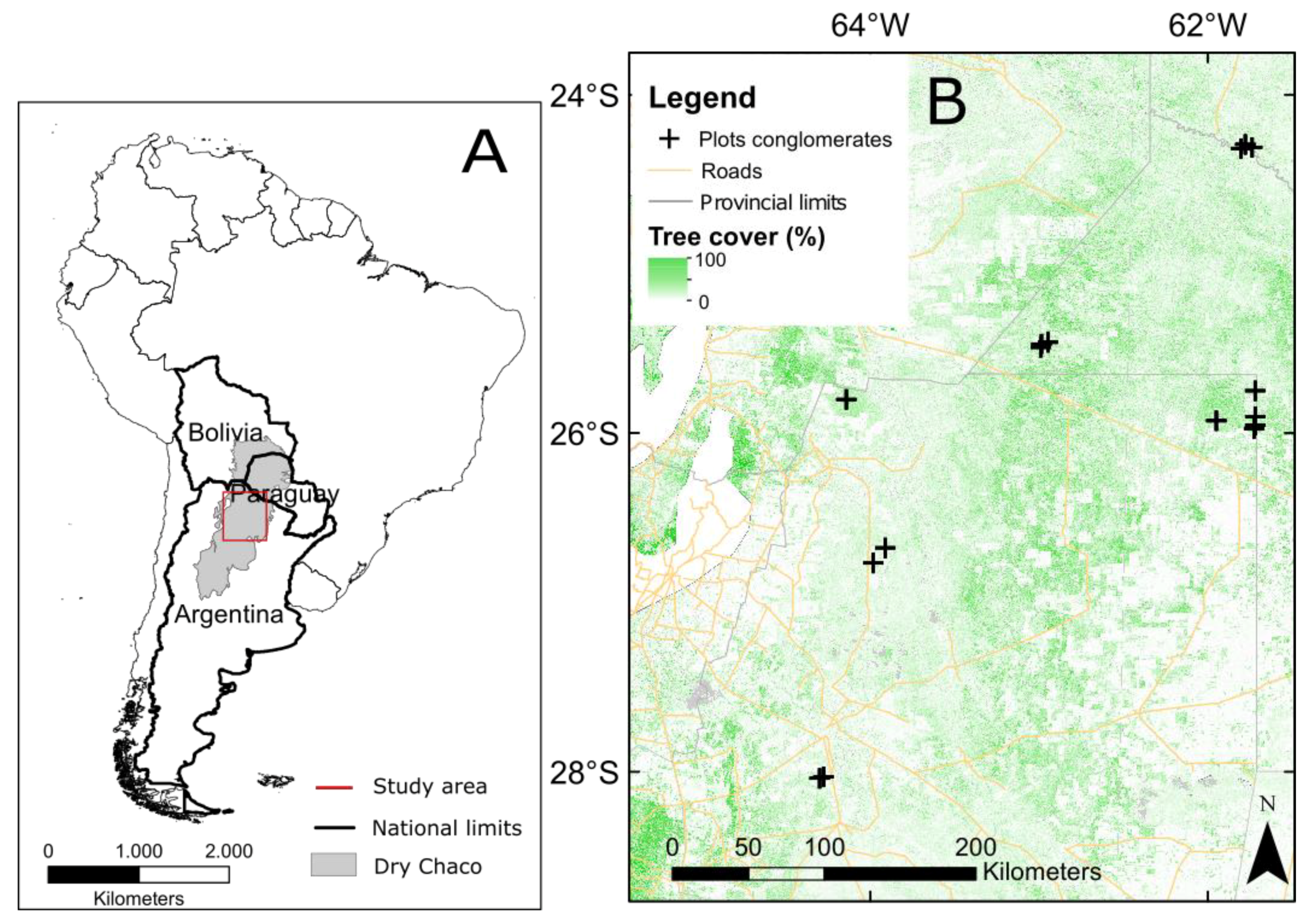
Figure 1. Location of the study sites: (A) the study area (red rectangle) situated in the central part of the Dry Chaco within South America, (B) the 16 clusters of 4 forest inventory plots. The map shows the average tree cover (%) derived from Landsat composites from the year 2015 [31].
Remotesensing 12 04005 g001
Figure 2. One cluster of four forest inventory plots of 1000 m2 each. For field data collection, the inventory plots are divided in two concentric circles, where all trees with breast height (DBH) > 0.1 m are documented for the inner circle of 500 m2 and only trees with DBH > 0.2 m for the outer circle. The background image is the orthophoto of the cluster that was reconstructed from the aerial photographs taken by the digital camera on the unmanned aerial vehicle (UAV).
Remotesensing 12 04005 g002
Figure 3. Extraction of information on canopy cover and vegetation openings based on the canopy height model for a given forest plot: (A) The polygons of canopy patches (green) and vegetation openings (red) are overlying the orthophoto taken by the UAV, (B) they are plotted on the canopy height model (CHM) of the same plot.
Remotesensing 12 04005 g003
Figure 4. Frequency distributions of the ground-based forest structure indicators. The indicators are described in Table 1, and summary statistics are given in Table 5.
Remotesensing 12 04005 g004
Figure 5. Frequency distributions of the forest structure indicators from the canopy height model and 3D point cloud of the UAV-SfM data. The indicators are described in Table 3 and Table 4, and summary statistics are given in Table 6.
Remotesensing 12 04005 g005
Figure 6. Comparison of the forest height indicators that were derived from the UAV-SfM data and the field-based measures of canopy height. The field data are plotted on the X-axis, while the UAV-SfM derived indicators are plotted on the Y-axis with the mean height of vegetation patches for (A) and the height of the tallest vegetation patch for (B). The Spearman correlation coefficients are calculated at the plot level (n = 40). If the p-value of the correlation analysis is less than 0.05, the correlation coefficient is flagged with one star (*).
Remotesensing 12 04005 g006
Figure 7. Comparison of forest structural indicators on vegetation density per stratum. The field data are plotted on the X-axis, while the UAV-SfM based indicators are plotted on the Y-axis. Panels A and B show the overall relative point density (ORD) in the 0.5 to 4 m stratum against respectively the percentage of trees in the same stratum and the percentage of trees with DBH < 0.2 m. Panels C and D show the same information for the 4 to 6 m stratum. The Spearman correlation coefficients are calculated at the plot level (n = 64). If the p-value of the correlation analysis is less than 0.05, the correlation coefficient is flagged with one star (*).
Remotesensing 12 04005 g007
Figure 8. The UAV-SfM data (n = 64) on vegetation openings, compared with ground measurements on the total tree density (ha−1) for panel A, and the density of trees (ha−1) with DBH < 0.2 m for panel B, between 0.2 and 0.3 m for panel C and > 0.3 m for panel D. The field data are plotted on the X-axis, while the UAV-SfM based indicator on vegetation openings is plotted on the Y-axis. The Spearman correlation coefficients are calculated at the plot level (n = 64). If the p-value of the correlation analysis is less than 0.05, the correlation coefficient is flagged with one star (*).
Remotesensing 12 04005 g008
Figure 9. The UAV-SfM data on canopy cover (%), compared with (A) ground measurements on the number of trees taller than 6 m (ha−1), and (B) the number of trees with DBH above 0.3 m. If the p-value of the correlation analysis is less than 0.05, the correlation coefficient is flagged with one star (*).
Remotesensing 12 04005 g009
Figure 10. Boxplots showing the distribution of four UAV-SfM structural indicators for the different classes of forest composition as they were defined in Table 1. The probability density at different values is smoothed by a kernel density estimator. The y-axis displays the structural indicators from the UAV-SfM products. The chi-squared (X2) from the Kruskal-Wallis test was implemented and if the p-value of the correlation analysis is less than 0.05, the correlation coefficient is flagged with one star (*). Groups with the different letters (a and b) are groups that are significantly different according to the pair-wise Wilcoxon test.
Remotesensing 12 04005 g010
Figure 11. Scatterplots relating all the forest indicators that were derived from the UAV-SfM data to the field-based measures of biomass (Mg/ha). The field data are plotted on the X-axis, while the UAV-SfM derived indicators are plotted on the Y-axis. The Spearman correlation coefficients are calculated at the plot level. If the p-value of the correlation analysis is less than 0.05, the correlation coefficient is flagged with one star (*).
Remotesensing 12 04005 g011
Table 1. Plot-level indicators on forest structure, composition, and function as they were derived from the field data on individual trees during the forest inventory. The above ground biomass is calculated with allometric equations using DBH values (expressed in cm) and the oven dry over green volume (p, in g/cm3).
Stand ElementVariableDescriptionUnit
STRUCTURETree heightMean height of upper canopyMean height of trees taller than 6 mm
Height tallest treeHeight of the tallest treem
Number of trees > 6 m Number   of   trees   taller   than   6   m Surface   area   of   the   plot ha−1
Percentage of trees in 0.5–4 m height stratum Number   of   trees   with   height   between   0.5   and   4   m Total   number   of   trees   in   the   plot × 100 %
Percentage of trees in 4–6 m height stratum Number   of   trees   with   height   between   4   and   6   m Total   number   of   trees   in   the   plot × 100 %
Tree spacingTree density Number   of   trees   in   the   plot Surface   area   of   the   plot ha−1
Tree diameter at breast height (DBH)Number of trees with DBH < 0.2 m Number   of   trees   with   DBH   <   0.2   m Surface   area   of   the   plot ha−1
Number of trees with 0.2 < DBH < 0.3 m Number   of   trees   with   0.2   m   <   DBH   <   0.3   m Surface   area   of   the   plot ha−1
Number of trees with DBH > 0.3 m Number   of   trees   with   DBH   >   0.3   m Surface   area   of   the   plot ha−1
Percentage of trees with DBH < 0.2 m Number   of   trees   with   DBH   <   0.2   m Total   number   of   trees   in   the   plot × 100 %
Percentage of trees with 0.2 < DBH < 0.3m Number   of   trees   with   0.2   <   DBH   <   0.3   m Total   number   of   trees   in   the   plot × 100 %
Percentage of trees with DBH > 0.3 m Number   of   trees   with   DBH   >   0.3   m Total   number   of   trees   in   the   plot × 100 %
COMPOSITIOSpeciesClassification based on dominant tree speciesCat 1: Aspidosperma quebracho-blanco, Schinopsis lorentzii, Bulnesia sarmientoi
Cat 2: Zizyphus mistol
Cat 3: Caesalpinia paraguariensis and Tabebuia nodosa
Cat 4: colonizer or pioneer species, like Prosopis nigra
FUNCTIONTree diameter and speciesAbove ground biomass (AGB)For trees with DBH < 0.6 m:
A G B = p × e 0.667 + 1.784 ln ( D B H ) + 0.207 ( ln ( D B H ) ) 2 0.0281 ( ln ( D B H ) ) 3
For trees with DBH > 0.6 m:
A G B   = p × e 1.589 + 2.284 ln ( D B H ) + 0.129 ( ln ( D B H ) ) 2 0.0197 ( ln ( D B H ) ) 3
Mg ha−1
Table 2. Camera, flight and imaging characteristics for all flights.
Camera modelPhantom 4 Pro camera
Lens modelFOV 84° (8.8 mm/24 mm) f/2.8–f/11
Image resolution5472 × 3648
Crop factor1
Approximate sensor size24 mm
Pixel size2.41 × 2.41 μm
Shutter speed8–1/8000 s
ISO Range100–3200
Mean f number2.8–11
Flight velocity2 m s−1
Flight height80–120 m
Ground sample distance21.8–45.3 mm
Number of pictures160–217
Point cloud density212–437 pt m−2
CHM resolution3.4–9.1 cm pix−1
Horizontal absolute accuracy2.6 m
Table 3. Derivation of forest structure indicators from the UAV-SfM (Unmanned Aerial Vehicle—Structure from Motion) images. The UAV-SfM data are converted to a canopy height model (CHM) and three-dimensional (3D) point cloud for the extraction of the forest structural indicators.
Data SourceProcessingIndicatorsUnits
Remotesensing 12 04005 i001
Canopy Height Model
Remotesensing 12 04005 i002
Canopy patches
Mean height of vegetation patches
Height of the tallest vegetation patch
Canopy cover
m
m
%
Remotesensing 12 04005 i003
Vegetation openings
Vegetation openings%
Remotesensing 12 04005 i004
Vegetation point cloud
Remotesensing 12 04005 i005
Height distribution of the point cloud
Stratum independent:
99th percentile
Vertical distribution
Vertical complexity


m
Stratum dependent:
Overall relative point density of 0.5 to 4 m stratum
Overall relative point density of 4 to 6 m stratum

%
%
Table 4. Plot-level indicators on horizontal and vertical forest structure, as they were derived from the canopy height model and 3D point cloud.
Forest StructureData SourceIndicatorDescriptionUnit
Horizontal complexityCHM (Vegetation data points)Mean height of tree crown patchesMean of the maximum heights of the tree crown patchesm
Height of the tallest vegetation patchMaximum height of the tallest canopy patchm
Canopy cover Surface   area   of   the   tree   crown   patches Total   surface   area   of   the   plot × 100 %
CHM (ground data points)Vegetation openings Surface   area   of   the   vegetation   openings Total   surface   area   of   the   plot   × 100 %
Vertical complexity3D point cloud (Percentile based)99th percentileHeight of 99th percentile of vegetation point cloudm
Vertical distribution Height   of   99 th   percentile     Height   of   50 th   percentile Height   of   99 th   percentile
Vertical complexity ( i = 1 HB p i ln p i ) / ln HB where pi is the proportional abundance of points within the height bin i; and HB is the total number of height bins of 1 m
3D point cloud (ORD based)Overall relative point density of 0.5 to 4 m stratum Number   of   points   between   0.5   and   4   m Total   number   of   points × 100 %
Overall relative point density of 4 to 6 m stratum Number   of   points   between   4   and   6   m Total   number   of   points × 100 %
Table 5. Summary of values for ground-based forest structure indicators, with indication of average, standard deviation, minimum and maximum values, and the number of plots where observations were made.
AverageS.D.Min.Max.# of Plots
Mean height of upper canopy10.31.87.516.140
Height tallest tree15.22.710.221.740
Number of trees > 6 m153.060.770.0300.040
Percentage of trees in 0.5–4 m height stratum10.416.50.064.140
Percentage of trees in 4–6 height stratum21.214.96.255.040
Tree density231.194.410056064
Number of trees with DBH < 0.2 m10786.8048064
Number of trees with 0.2 < DBH < 0.3m6029.92014064
Number of trees with DBH > 0.3 m4218.609064
Dominant species by classification----64
Above ground biomass (AGB)30.011.312.862.964
Table 6. Summary of values for UAV-SfM indicators, with indication of average, standard deviation, minimum and maximum values, and the number of plots where observations were made.
AverageS.D.Min.Max.# of Plots
Mean height of vegetation patches8.11.26.111.264
Height of the tallest vegetation patch12.82.46.917.664
Canopy cover25.610.82.856.664
Vegetation openings8.38.10.034.364
99th percentile11.32.25.91664
Vertical distribution0.70.10.40.964
Vertical complexity0.70.10.50.864
ORD of 0.5 to 4 m stratum50.215.214.782.364
ORD of 4 to 6 m stratum15.99.52.647.564
Publisher’s Note: MDPI stays neutral with regard to jurisdictional claims in published maps and institutional affiliations.