Abstract
This study provided a comprehensive evaluation of eight machine learning regression algorithms for forest aboveground biomass (AGB) estimation from satellite data based on leaf area index, canopy height, net primary production, and tree cover data, as well as climatic and topographical data. Some of these algorithms have not been commonly used for forest AGB estimation such as the extremely randomized trees, stochastic gradient boosting, and categorical boosting (CatBoost) regression. For each algorithm, its hyperparameters were optimized using grid search with cross-validation, and the optimal AGB model was developed using the training dataset (80%) and AGB was predicted on the test dataset (20%). Performance metrics, feature importance as well as overestimation and underestimation were considered as indicators for evaluating the performance of an algorithm. To reduce the impacts of the random training-test data split and sampling method on the performance, the above procedures were repeated 50 times for each algorithm under the random sampling, the stratified sampling, and separate modeling scenarios. The results showed that five tree-based ensemble algorithms performed better than the three nonensemble algorithms (multivariate adaptive regression splines, support vector regression, and multilayer perceptron), and the CatBoost algorithm outperformed the other algorithms for AGB estimation. Compared with the random sampling scenario, the stratified sampling scenario and separate modeling did not significantly improve the AGB estimates, but modeling AGB for each forest type separately provided stable results in terms of the contributions of the predictor variables to the AGB estimates. All the algorithms showed forest AGB were underestimated when the AGB values were larger than 210 Mg/ha and overestimated when the AGB values were less than 120 Mg/ha. This study highlighted the capability of ensemble algorithms to improve AGB estimates and the necessity of improving AGB estimates for high and low AGB levels in future studies.
1. Introduction
Forest biomass is an essential climate variable that measures the net carbon dioxide exchange between the land surface and the atmosphere [1]. Accurate estimation of forest biomass and its changes can enhance our understanding of the global carbon cycle as well as reduce the uncertainties of estimated carbon emissions resulting from anthropogenic activities or natural disturbances [2,3,4,5,6,7,8]. The living forest biomass carbon pool consists of aboveground biomass (AGB) and belowground biomass (BGB), but in most cases, forest biomass is referred to as AGB, which is measurable with some accuracy at a broad scale; BGB is often derived from AGB using root–shoot ratios [1,9,10].
There is widespread consensus among studies that forest AGB can be best estimated from a combination of field measurements and remotely sensed datasets. Based on both types of data, many forest AGB maps were produced at local, regional, or global scales using various algorithms [2,3,4,5,6,7,8]. However, due to the uncertainties associated with the selection of allometric equations to calculate field biomass and the uncertainties in remote sensing datasets and the algorithms used for AGB prediction, substantial uncertainties remain in current AGB estimates [11,12,13]. To improve the accuracy of AGB estimation, some recent studies have proposed that efforts should be made to compile field biomass extensively, integrate multiple remote sensing datasets, explore novel approaches, and comprehensively address the uncertainty associated with biomass estimates [11,14,15,16].
With respect to approaches for forest AGB estimation, machine learning regression algorithms received a lot of attention over the past decades [17,18,19]. These include the classification and regression tree (CART) learner [20] and its extensions using bagging or boosting techniques, followed by the development of random forests (RFs) and the gradient-boosted regression tree (GBRT) algorithm [7,21,22,23]. In addition to RFs and the GBRT, the support vector regression (SVR) method [24,25], artificial neural networks (ANNs) [17], maximum entropy (MaxEnt) algorithm [5], k-nearest neighbors (kNN) method [26], and multivariate adaptive regression splines (MARS) algorithm [27,28] have been commonly used in the estimation of forest AGB. There are also some studies that compared the performances of these algorithms in retrieving forest AGB. For example, Wu et al. [29] compared the stepwise linear regression, kNN, SVR, RF, and stochastic gradient boosting (SGB) approaches for estimating forest AGB from Landsat images in northwestern Zhejiang Province, China, and found that the RF exhibited the best performance. Almeida et al. [24] assessed the performances of a linear model, a linear model with ridge regularization, SVR, RF, SGB, and the cubist model to estimate AGB from airborne lidar and hyperspectral imaging in the Brazilian Amazon. The results suggested that the linear models performed poorly and that no regression model outperformed the others. Pham et al. [30] evaluated the capabilities of the GBRT, SVR, RF, categorical boosting (CatBoost) regression, and their proposed extreme gradient boosting decision tree technique together with a genetic algorithm for feature selection (XGBR-GA) for estimating mangrove AGB from multiple data sources and found that XGBR-GA outperformed the other four machine learning models.
Although these above studies have examined or compared the performances of machine learning algorithms for estimating AGB, they were mainly limited to several commonly used algorithms. Some algorithms, such as the extremely randomized trees (ERT) and CatBoost methods, have attracted much attention in the machine learning community and have outperformed commonly used algorithms when applied in other fields [31,32], but their performances for AGB estimation have not been fully investigated. Moreover, recent studies mainly focused on the overall accuracy of estimated AGB, and the problems of overestimation and underestimation when estimating AGB with an inversion algorithm were largely ignored [21]. A few studies have indicated that the overestimation or underestimation of AGB could depend on the AGB ranges or AGB values of training samples, but it is still unclear how the accuracy of estimated AGB varies with the AGB values [33].
The objectives of this study are to evaluate newly proposed or not commonly used algorithms (e.g., ERT, SGB, CatBoost) for AGB estimation and explore how they perform in comparison with established models, such as the MARS, RF, SVR, GBRT, and ANN algorithms, and to investigate how the performances of these machine learning regression algorithms for AGB estimation from multiple satellite data products vary with the AGB ranges.
2. Overview of Machine Learning Regression Algorithms
This section presents a brief overview of the machine learning techniques used for the evaluation. Since the objective of this study is to examine the performances of machine learning algorithms for estimating forest AGB, this overview is not a detailed explanation of each algorithm but rather a summary. Both the approaches established and some algorithms yet to be tested for AGB estimation are included.
2.1. Linear-Based Learners
Linear regression and its extensions are simple algorithms used for the estimation of land surface variables from remote sensing data. Due to the multicollinearity between predictor variables obtained from remote sensing data, linear regression cannot be directly used to estimate forest biomass [24]. Therefore, some studies have performed stepwise regression to select the optimal independent variables for AGB estimation or used partial least-squares regression, which first reduces the predictors to a small set of uncorrelated components and then performs least-squares regression on these components to estimate forest AGB [21]. However, because of the nonlinear relationships between the predictors and forest biomass, the estimated forest AGB is usually inaccurate [34]. Compared with these linear models, the MARS method can capture nonlinear relationships by creating piecewise-linear models and thus provides higher accuracy for AGB estimates [35,36]. For this reason, the MARS algorithm was selected in this study.
2.2. Kernel-Based Learners
Kernel-based learners are a family of algorithms that use kernel functions to project low-dimensional data to a higher dimension to make them linearly separable. They deal with nonlinear problems while still operating with linear algebra [37]. SVR is a kernel-based algorithm commonly used for retrieving biophysical parameters from remote sensing data [38], and it was proven to have good performance in estimating forest AGB [21,39]. Gaussian processes regression (GPR) is another kernel-based algorithm that establishes the relationships between predictor variables and forest biomass in the same way as SVR [37,40]. GPR is a nonparametric Bayesian approach, and it can provide not only the predicted mean value for the estimation but also the variance [41]. Previous studies have suggested that both SVR and GPR are suitable for estimating forest structure parameters but that GPR is slightly more accurate than SVR [37]. In addition to SVR and GPR, kernel ridge regression (KRR) is also a kernel-based algorithm that combines ridge regression and the kernel trick. KRR learns a model quickly for medium or large datasets. Previous studies used KRR for estimating biophysical parameters, such as leaf chlorophyll content, leaf area index, and fractional vegetation cover, and compared its performance with those of SVR and GPR [41], but KRR has not yet been applied in forest AGB estimation.
2.3. Tree-Based Models
Tree-based learners have been widely used in parameter estimation due to their efficiency and reliability [23,42]. To date, two types of tree-based learners have been used for estimation: individual tree-based models (e.g., CART and C4.5) and their extensions using bagging or boosting [20,43,44]. For an individual tree-based model, small changes in the learning sample can cause dramatic changes in the built tree, and so the estimated results in previous studies were unstable and inaccurate [45,46]. To improve this situation, most studies adopted bagging and boosting ensemble algorithms. The bagging process in tree-based models applies bootstrap samples generated from the original dataset to train tree models and then aggregates the ensembles to obtain final predictions [47]. Through aggregation, bagging algorithms improve the predictions by decreasing variance [48]. RF is a modified version of the bagging algorithm that builds trees using not only subsamples but also a random subset of predictors to determine each split, and this technique can reduce the correlations between different prediction ensembles [49]. Due to its robustness to overfitting and noise in the training dataset, RF can be very effective for estimating parameters such as forest AGB [21,22]. Approximately 30% of training samples are not included in the modeling of the RF algorithm because of bootstrapping and resamples and can be applied to compute the out-of-bag prediction error.
The ERT algorithm is another tree-based ensemble algorithm that improves the accuracy parameter estimation by reducing variances. Different from other tree-based ensemble methods, the ERT algorithm splits nodes by choosing cut points completely at random and uses the whole learning sample rather than a bootstrap replica to grow the trees [48,50]. Since it does not require the determination of optimal discretization thresholds, the ERT algorithm has an advantage in terms of computing time. To date, the ERT algorithm was utilized to predict terrestrial latent heat fluxes [31], air quality [51], and streamflow models [52], but its performance in estimating forest AGB has not yet been explored.
Boosting is a family of sequential ensemble algorithms that converts weak learners to strong learners, thereby eventually improving the prediction accuracy by decreasing bias [53]. Boosting algorithms pay the most attention to the samples with the highest prediction errors and increase their weights in the next iteration. The final prediction results are a weighted combination of predictions across the sequence of learners. The gradient boosting machine (GBM) is an extremely popular boosting algorithm and one of the leading algorithms for winning Kaggle competitions. For a GBM, the base learners are decision trees. Despite being popular in the machine learning community, the GBM and GBRT approaches are rarely applied in forest AGB estimation studies [23,30]. SGB is another implementation of the tree-based gradient boosting approach that builds a base learner from a random subsample drawn from the entire training dataset without replacement at each iteration, and it can thus reduce the risk of overfitting [54,55]. Moisen et al. [56] illustrated the use of SGB in mapping the presence and basal area of 13 species. Filippi et al. [57] adopted SGB to estimate floodplain-forest AGB from hyperspectral Hyperion images and ancillary data. CatBoost is a new version of the GBRT [58]. As the name suggests, CatBoost can address categorical variables. The implementation of ordered boosting is another critical algorithmic advance in CatBoost [59]. Huang et al. [60] evaluated the CatBoost method for the prediction of reference evapotranspiration in humid regions and found that CatBoost could perform better than the RF and SVM models.
As addressed above, a series of bagging and boosting ensemble algorithms were proposed to increase the accuracy of estimated parameters, but their applications in AGB prediction are very rare. Therefore, ensemble algorithms, including the RF, ERT, GBRT, SGB, and CatBoost were chosen for comparison in this study.
2.4. Neural Network-Based Learners
Neural networks have attracted great attention in recent years. Inspired by biological neural networks, ANNs have been used to construct nonlinear models between independent variables and dependent variables, emulating the learning of the biological neuron system [61]. The basic model of an ANN consists of one input layer, one or more hidden layers, and one output layer. The feedforward multilayer perceptron (MLP) model has been the most widely used ANN model in various fields since the introduction of the back propagation algorithm and is also an alternative approach for reliable forest biomass prediction [62,63,64,65]. The extreme learning machine (ELM) is a novel type of ANN with a single hidden layer, where the hidden nodes are randomly initiated and then fixed without iteratively tuning them [66,67]. Empirical studies suggested that the efficiency and generalization abilities of the ELM are comparable to or even better than those of the SVR algorithm [67,68]. Variations in the ELM were developed to make it more suitable for specific applications [69], but it has not yet been extended for forest AGB estimation.
3. Data and Methods
3.1. Reference AGB Data
The reference AGB data are indispensable for forest AGB estimation from satellite datasets. They have often been used to calibrate remote sensing datasets and validate the estimated results. In this study, the reference AGB data were compiled from field AGB and high-resolution AGB datasets that were originally derived from field data and lidar data [70]. The field AGB data were obtained by collecting plot-level AGB that were measured on or after the year 2000 from published literature and online databases. To increase the number of training samples, high-resolution AGB datasets with spatial resolutions finer than 100 m that could match well with field AGB at the spatial scale were also considered. Both field AGB and high-resolution AGB datasets were aggregated to 0.01°. More details about the sources and preprocessing of plot-level AGB and high-resolution AGB datasets to generate the reference AGB data can be found in one of our previous papers [71].
Since the relationships between forest AGB and predictor variables may vary with forest types, we separated the reference AGB data with the MODIS (Moderate Resolution Imaging Spectroradiometer) Land Cover Type Product (MCD12Q1, version 6) for 2005 and the International Geosphere-Biosphere Programme (IGBP) legend [72]. A total of 12,376 reference AGB samples at 0.01° resolution were finally selected, including 249 samples located in evergreen needleleaf forests (ENFs), 1600 samples in evergreen broadleaf forests (EBFs), 3689 samples in deciduous broadleaf forests (DBFs), 585 samples in mixed forests (MFs), 4993 samples in woody savannas (WSAs), and 1260 samples in savannas (SAVs) (Figure 1). The AGB samples corresponding to non-forest types according to the MCD12Q1 for 2005 were excluded. The statistics of the reference AGB samples sorted by forest type are shown in Table 1.
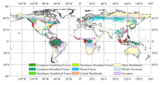
Figure 1.
The spatial distribution of reference aboveground biomass (AGB) data. The background map shows the forest types according to the International Geosphere-Biosphere Programme classification based on MCD12Q1 data for 2005.

Table 1.
Statistics of the reference AGB samples used in this study.
3.2. Input Data Collection
It was demonstrated that the multisensor synergy of optical, radar, and lidar data could improve the accuracy of AGB estimation [4,73,74,75,76]. Previous studies generally incorporated high-level satellite data products that were originally derived from optical, radar, and lidar data, or a combination of them, into the process of estimating AGB based on satellite observations. In this study, the satellite data products included were the Global Land Surface Satellites (GLASS) leaf area index (LAI), canopy height derived from the Geoscience Laser Altimeter System (GLAS) data, MODIS net primary production (NPP), as well as tree cover data derived from Landsat images, which were closely correlated with forest AGB under some conditions [42,77,78]. In addition, climatic and topographical factors could significantly or marginally improve the accuracy of forest AGB estimates and thus served as predictor variables of forest AGB in this study [79,80,81,82,83].
3.2.1. GLASS LAI Data
As part of the GLASS products suite [84], the GLASS LAI product at 8-day and 1-km resolutions was used because it is more accurate and temporally continuous than other LAI products such as MODIS LAI and Geoland2 LAI [85,86,87]. The 8-day GLASS LAIs from 2001 to 2010 were first reprojected to the WGS 84 geographic coordinate system and then averaged at the monthly scale. The maximum monthly LAI value within a year was taken as the annual maximum LAI. Here, we used the annual maximum LAI for the year 2005 and the interannual variation in LAI, which was represented by the coefficient of variation (CV) of the annual maximum LAIs from 2001 to 2010.
3.2.2. Global Canopy Height Map
The global canopy height map at 1-km resolution was derived from the GLAS data compiled in 2005 by Simard et al. [88]. Compared with the global height map produced by Lefsky [89], the Simard et al. [88] product was in better agreement with airborne lidar-derived heights [90]. Therefore, the Simard et al. [88] global canopy height map was used to extract the canopy height, which was a predictor of forest AGB. For consistency with other datasets, we resampled the canopy height map to 0.01° using the nearest neighbor method.
3.2.3. MODIS NPP Data
The MODIS annual NPP data are one of the most highly used data sources for studies on the global carbon cycle [91]. The annual MOD17A3HGF (version 6) data at 500-m resolution, provided in a sinusoidal projection, were downloaded from the Land Processes Distributed Active Archive Center (https://lpdaac.usgs.gov/products/mod17a3hgfv006) [92]. Annual NPP data from 2001 to 2010 were converted to the WGS84 geographic coordinate system with the MODIS Reprojection Tool and then aggregated to 0.01°. Like the LAI data, annual NPP data for 2005 and the interannual variation in NPP from 2001 to 2010 were included.
3.2.4. Global Tree Cover Product
The global forest cover map at 30-m spatial resolution for 2000 generated by Hansen et al. [93] was used. To be consistent with other datasets, the 30-m data were aggregated to 0.01° resolution. The standard deviation of all 30 pixels within each 0.01° grid cell was also extracted to describe the spatial variability of tree cover [94].
3.2.5. Global Multi-Resolution Terrain Elevation Data 2010 (GMTED2010)
The DEM and slope data were extracted from the GMTED2010 product, which covered global land areas from 84°N to 56°S [95]. The GMTED2010 product was mainly constructed from the SRTM data. For regions outside the coverage area of the SRTM, 10 other elevation datasets, such as the GTOPO30 dataset, Canadian digital elevation data, and the National Elevation Dataset for the continental United States and Alaska, were used to fill the gaps. The GMTED2010 suite contains raster elevation products at 30, 15, and 7.5 arc-second spatial resolutions. Here, we used the GMTED2010 data at 30 arc-second spatial resolution, which had a lower RMSE range between 25 and 42 m with respect to a global set of control points provided by the National Geospatial-Intelligence Agency than the 66 m RMSE of GTOPO30 relative to the same control points.
3.2.6. Climate Data
The WorldClim2 dataset at 1-km spatial resolution provided monthly temperature (minimum, maximum, and average) and precipitation information for global land areas during the period of 1970–2000 and could be downloaded from http://worldclim.org/version2 [96]. The monthly average temperature and precipitation data were aggregated to the annual scale and used in this study.
The Climatic Research Unit (CRU) gridded dataset contains monthly time series of temperature and precipitation data from 1901 to the present day [97]. Monthly temperature and precipitation data from 2001 to 2010 were aggregated to the annual scale, and changes in annual temperature and precipitation were derived by standardizing the data during the period of 2001–2010 to the baseline period (1971–2000), and then they served as predictor variables of forest AGB.
3.3. AGB Modeling Algorithms
Based on the reference AGB data and their corresponding predictor variables that were extracted from multiple satellite data products and the ancillary climatic and topographical datasets, forest AGB was estimated with eight machine learning algorithms. Thirteen variables were selected as predictor variables, including the LAI, interannual variation in LAI (LAI-CV), canopy height (CH), NPP, interannual variation in NPP (NPP-CV), tree cover (TC-Mean), standard deviation of tree cover within each 0.01° grid (TC-Std), DEM, slope, temperature (Temp), changes in temperature (Temp-Anomaly), precipitation (Prec), and changes in precipitation (Prec-Anomaly). The eight nonparametric regression algorithms included the MARS algorithm, a kernel-based model (SVR), a neural network-based model (MLP), and five tree-based ensemble models including the RF, ERT, GBRT, SGB, and CatBoost approaches. The modeling of forest AGB with the SVR, RF, ERT, GBRT, SGB, and MLP approaches was implemented with the scikit-learn machine learning library for the Python programming language [98]. The MARS and CatBoost algorithms were implemented with the py-earth and catboost libraries, respectively.
3.3.1. Tuning the Hyperparameters for the Machine Learning Algorithms
The hyperparameters of an algorithm affect its performance when estimating forest AGB. It is essential to optimize the hyperparameters of each algorithm before conducting any further evaluation or comparison of these algorithms. The key tuning hyperparameters and the configurations of the tuning parameters for each algorithm are shown in Table 2.
Table 2.
Hyperparameters tuned and their configurations for each algorithm.
For the MARS algorithm, the hyperparameters are the maximum number of terms to retain in the final model (max_terms) and the maximum degree of the interactions between piecewise linear functions (max_degrees). The radial basis function was selected as the kernel for SVR because it could capture the nonlinear relationships between the predictors and forest AGB. The regularization parameter C and kernel coefficient gamma were tuned for SVR-RBF. The parameter C controls the trade-off between the slack variable penalty (misclassifications) and the width of the margin, while gamma determines how much influence a single training sample exerts. For the five tree-based AGB modeling algorithms, the number of trees to build (n_estimators) must be tuned. The RF algorithm also requires the tuning of the number of features to consider when splitting a node (max_features). For the ERT method, two hyperparameters were optimized for the splitting procedure: the number of features randomly selected at each node (max_features) and the minimum sample size required to split a node (min_samples_split). For the three boosting algorithms, GBRT, SGB, and CatBoost, the learning rate determined the contribution of each regression tree and was therefore tuned. In addition to the number of trees to build and the learning rate, the tuning parameters in the GBRT model included the minimum sample size required to split an internal node (min_samples_split) and the maximum depth of a tree (max_depth), which controls the complexity of each individual tree. Compared with the GBRT algorithm, the fraction of samples (subsample) that were randomly selected to build each tree was added to the set of hyperparameters of SGB. The hyperparameters of the CatBoost algorithm include the learning rate, the depth of the tree (depth), and the maximum number of trees (iterations) that can be built [59]. For the MLP model, the size of the hidden layer (hidden_layer_sizes), which includes both the number of hidden layers and the number of perceptrons contained in each hidden layer, must be tuned.
Based on the hyperparameter configurations shown in Table 2, the optimal combination of hyperparameters for each AGB model was determined using grid search with cross-validation. The procedure of tuning the hyperparameters for a given algorithm is shown in Figure 2. The initial data were divided into a training dataset (80%) and a test dataset (20%). Five-fold cross-validation was employed to optimize the hyperparameters; the training data were divided into five folds, with four folds chosen for training the AGB model and the remaining fold held out for validation. Each of the five folds acted once as a validation set and four times as a training set. The root mean square error (RMSE) was calculated based on the validation set. The optimal combination of hyperparameters had the minimum average RMSE for the five validation datasets. Once the optimal hyperparameter combination was determined for an AGB modeling algorithm, the corresponding hyperparameters were set for the model. All the training data were then used to train the AGB model, and 20% of the test data were used to evaluate its performance for AGB estimation. To ensure that the comparison results of different AGB modeling algorithms were stable and not subject to the splitting of the training and test datasets, the procedures for tuning the hyperparameters of an AGB model and evaluating model performance were repeated 50 times, randomly splitting the training set and test set compositions each time (Figure 2). Ten to a hundred times were usually adopted. Considering the running time, the random splitting was repeated 50 times in this study. The performance metrics calculated on the 50 test sets were all stored, and the average of the 50 performance metrics was also calculated to evaluate the performance of each AGB modeling algorithm.
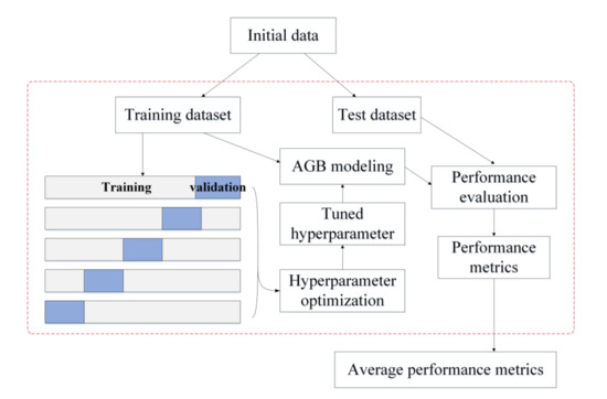
Figure 2.
Experimental design for tuning hyperparameters and evaluating an AGB modeling algorithm.
3.3.2. AGB Modeling under Different Scenarios
To fully investigate the performances of eight machine learning regression algorithms for AGB estimation from multiple satellite datasets and ancillary information, the following scenarios were designed.
- (1)
- AGB models were developed based on the random sampling of initial data without stratification of forest types, resulting in a total of 8 models for examination;
- (2)
- AGB models were built based on the random sampling of initial data with stratification of forest types, producing 8 models under stratified sampling scenarios;
- (3)
- AGB models were developed for each forest type separately based on the random sampling of initial data for the corresponding forest type, which led to a total of 48 models for evaluation (8 models for each forest type).
The second scenario was designed to address whether, compared with the random sampling scenario, the stratification of forest types could improve the accuracy of AGB estimation achieved by eight machine learning algorithms. The training dataset under the stratified sampling scenario was the same as the sum of the training datasets of the six AGB models developed separately for each forest type. The comparison results under the second and third scenarios illustrated whether the separate modeling of AGB improved the forest AGB estimates with these machine learning algorithms.
As addressed in Section 3.3.1, each of the 64 AGB models under the above three scenarios were first optimized based on the training data using grid search with cross validation, then they were developed with the whole training dataset, which accounted for 80% of the whole data, and finally they were evaluated with the remaining 20% of the test data. The procedure was repeated 50 times for each AGB model.
3.4. Performance Evaluation of the AGB Models
The performance of each AGB model was evaluated using four commonly used indicators, including the coefficient of determination (R2), root mean square error (RMSE), relative RMSE (RMSE%), and bias. These metrics can be calculated as follows:
where is the reference AGB, is the average of the reference AGB values, and is the estimated AGB. N is the number of test samples used for the evaluation. High R2 values were preferred, while lower values of the RMSE, relative RMSE, and bias indicated better performance by an AGB model.
3.5. Comparison Analysis of the Algorithms for Modeling AGB
The overall performances of the AGB models under the three scenarios were evaluated in terms of their R2, RMSE, bias, and relative RMSE values. For each AGB-modeling algorithm, the performance metrics for 50 runs were calculated. In addition to the performance metrics calculated based on the whole test data for each run, the performances for each forest type were computed using the test data with their corresponding forest types. Only the stratified sampling scenario and separate modeling scenario were considered when we explored how the eight algorithms performed for AGB estimation of each forest type, since these two scenarios used the same training data and test data for AGB modeling and performance evaluation.
Among the eight algorithms, the MARS, RF, ERT, GBRT, SGB, and CatBoost methods provided the coefficients measuring the contributions of the prediction variables in the various AGB models. The base model of the RF, ERT, GBRT, SGB, and CatBoost algorithms was the CART model, and the mean decrease in impurity importance was used to rank the importance of features [99]. In the MARS algorithm, the contribution of each predictor was determined using the generalized cross-validation statistic [100,101]. The feature importance values for the six models were calculated for 50 runs, and the distribution of the feature importance values for each model was represented by the mean, minimum and maximum values.
In addition to the overall performance metrics and feature importance values for 50 runs, we compared the performances of the eight AGB modeling algorithms in terms of AGB prediction under three scenarios. Some of the initial data acted as the test set multiple times for 50 runs. We combined the predictions for 50 runs of each algorithm using two approaches. One approach was to simply combine all the predictions (20% of the initial data for each run, with 50 runs) without integrating the predicted values corresponding to the same test samples; this approach generated 123,800 predictions for each algorithm. The other approach was to integrate the predicted values corresponding to the same samples; this approach produced 12,376 predictions for each algorithm. Based on the generated AGB estimates and the corresponding reference AGB, we compared the performances of all eight AGB modeling algorithms. Following this, we calculated the prediction errors (predicted value minus the reference AGB) of each algorithm and explored the relationship between the prediction errors and the reference AGB. Moreover, the AGB predictions were separated into eight bins according to the reference AGB: 0 < reference AGB ≤ 60 Mg/ha, 60 < reference AGB ≤ 90 Mg/ha, 90 < reference AGB ≤ 120 Mg/ha, 120 < reference AGB ≤ 150 Mg/ha, 150 < reference AGB ≤ 180 Mg/ha, 180 < reference AGB ≤ 210 Mg/ha, 210 < reference AGB ≤ 240 Mg/ha, and reference AGB > 240 Mg/ha. The prediction errors within each bin were calculated, and the results from different algorithms were compared to comprehensively explore the underestimation and overestimation of AGB by eight machine learning regression algorithms.
4. Results
4.1. Performance Metrics for the Optimized AGB Models
Figure 3 shows the distribution of the validated R-squared, RMSE, bias, and relative RMSE results for 50 runs of each regression algorithm under three scenarios. The five tree-based ensemble algorithms, RF, ERT, GBRT, CatBoost, and SGB, outperformed the SVR, MLP, and MARS algorithms in terms of the R-squared, RMSE, and relative RMSE values. SVR produced the AGB estimates with the largest bias and significantly underestimated forest AGB (Figure 3c and Table 3). Averaging the performance metrics of 50 runs for each regression algorithm, we found that the CatBoost algorithm had the overall best performance in estimating forest AGB from multiple satellite data products, with a mean R-squared of 0.71, RMSE of 46.67, and relative RMSE of 26% (Table 3). In contrast, the MARS model achieved the lowest mean R-squared at 0.56, the highest RMSE at 56.69 Mg/ha, and a relative RMSE of 31.58%.
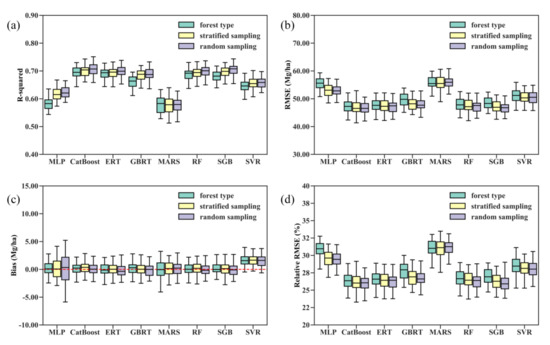
Figure 3.
Distribution of the 50 validated (a) R-squared, (b) RMSE, (c) bias, and (d) relative RMSE values for each machine learning regression algorithm under three modeling scenarios. Random sampling corresponds to AGB modeling without stratification of forest types, stratified sampling corresponds to AGB modeling with stratification of forest types, and forest type corresponds to separate AGB models for each forest type scenario.
Table 3.
Average performance metrics for the 50 runs of each regression algorithm under the random sampling scenario.
The comparison results of the performances of the eight machine learning regression algorithms did not vary with the training datasets used. In other words, the random splitting of the training and test data did not greatly affect the performance metrics obtained by the AGB modeling algorithms, particularly the tree-based ensemble algorithms. Additionally, the modeling scenarios did not change the comparison results. Both stratified random sampling and modeling AGB for each forest type separately did not improve the overall accuracy of the AGB estimates obtained by the eight algorithms (Figure 3).
Compared with the MLP and MARS algorithms, the performances of the RF, ERT, GBRT, CatBoost, and SGB approaches were more stable and less sensitive to the training datasets and modeling scenarios. The mean biases for 50 runs each of the RF, ERT, GBRT, CatBoost, and SGB approaches were −0.03 Mg/ha, −0.21 Mg/ha, −0.11 Mg/ha, −0.07 Mg/ha, and 0.10 Mg/ha, respectively, and the median biases were −0.15 Mg/ha for the RF, −0.36 Mg/ha for the ERT model, −0.01 Mg/ha for the GBRT, −0.09 Mg/ha for SGB and 0.03 Mg/ha for the CatBoost algorithm under the random sampling scenario (Figure 3 and Table 3). The results suggested that the RF, ERT, GBRT, and SGB models generally overestimated forest AGB, while the CatBoost algorithm slightly underestimated forest AGB.
Comparing the performances of the eight algorithms for estimating the AGB of different forest types under the stratified sampling scenario and separate modeling scenario, we found that modeling AGB for each forest type separately did not improve the accuracy of the AGB estimates but instead resulted in large variations in the bias and relative RMSE values due to the random splitting of the training data and test data for each of the 50 runs (Figure 4). One exception was that the MARS algorithm developed for the mixed forests had a good performance with a corresponding median bias close to zero, while the MARS model built under the stratified sampling scenario showed an overestimation of AGB in mixed forests.
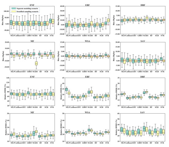
Figure 4.
Distribution of 50 validated biases and relative RMSEs for eight AGB modeling algorithms under the stratified sampling scenario and separate modeling scenario.
Large discrepancies in the bias and relative RMSE values were observed for the different algorithms. However, all the AGB modeling algorithms achieved good performances in estimating the AGB of DBFs, with relative RMSEs ranging from approximately 15 to 25% and biases ranging from −5.0 to 5.0 Mg/ha, but they achieved poor performances in estimating the AGB of ENFs with relative RMSEs larger than 60%. A possible reason for the poor accuracy of the predicted AGBs of ENFs was that many ENF samples had high AGB values, which could not be captured by the satellite data products due to saturation problems (Table 1). For EBFs, all the regression algorithms except SVR underestimated AGB under the stratified sampling scenario while overestimating AGB under the separate modeling scenario. In contrast, the regression algorithms with stratified sampling overestimated the AGB of MFs and WSAs, while the separate AGB models provided underestimated AGB values (Figure 4).
Under either scenario, the MLP, MARS, and SVR models were not optimal for all forest types (Figure 4). Although the five tree-based ensemble algorithms, including the RF, ERT, GBRT, SGB, and CatBoost algorithms, had better performances than the MLP, MARS, and SVR models, no single tree-based algorithm was optimal for all forest types (Figure 5). The RF, ERT, GBRT, and SGB models had similar performances in terms of AGB estimation when modeling AGB separately for the EBF, DBF, MF, WSA, and SAV types. For ENFs, the ERT algorithm provided relatively better results than those of the other algorithms, but only under the separate modeling scenario.
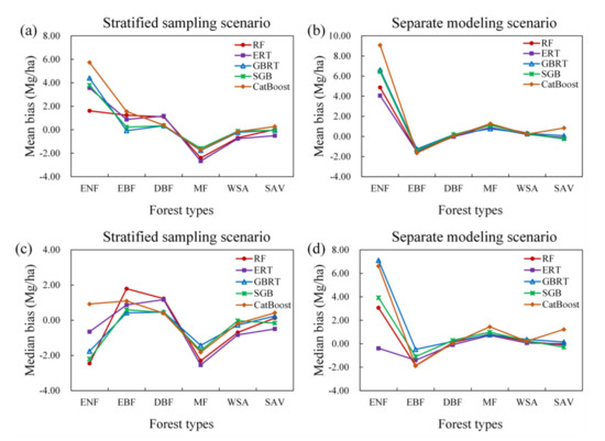
Figure 5.
Comparison results of the performances of five tree-based ensemble algorithms (RF, ERT, GBRT, SGB, and CatBoost) for AGB estimates of different forest types in terms of bias under the stratified sampling scenario (a,c) and separate modeling scenario (b,d).
4.2. Relative Importance of the Predictor Variables in AGB Models
Figure 6 shows that the relative importance values of 13 predictor variables in different AGB modeling algorithms were different. For the RF, GBRT, and SGB models, the CH contributed the most to AGB estimation, with different values of feature importance. TC-Mean was the most important variable for estimating AGB using the MARS algorithm. However, its contributions were greatly affected by the training data used and varied from 10.35 to 59.65%. For the ERT and CatBoost algorithms, TC-Mean also contributed more to the AGB predictions than the other predictor variables, with corresponding importance values ranging from 11.58 to 16.74%.
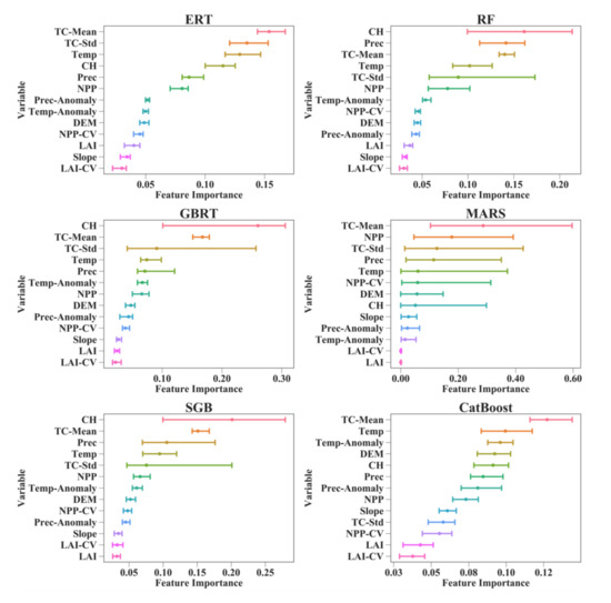
Figure 6.
Feature importance values for the predictor variables in eight machine learning regression algorithms under the random sampling scenario. The lines connect the corresponding minimum and maximum feature importance values for 50 runs of each predictor variable, and the points represent the average of the 50 feature importance values for each predictor variable. CH is the canopy height; Prec is the precipitation; Prec-Anomaly is the changes in precipitation; LAI is the leaf area index; LAI-CV is the interannual variation in LAI; NPP is the net primary production; NPP-CV is the interannual variation in NPP; TC-Mean is the mean tree cover within each 0.01° grid cell; TC-Std is the standard deviation of tree cover within each 0.01° grid cell; DEM is the digital elevation model; Temp is the temperature; and Temp-Anomaly is the changes in temperature.
Compared with the MARS, RF, GBRT, and SGB models, the ERT and CatBoost algorithms provided more stable results in terms of the importance of the predictor variables to AGB estimation. This was established under both the random sampling and stratified sampling scenarios (Figure 6 and Figure S1). The changes in feature importance values caused by the random splitting of the training sets and test sets for each of the 50 runs were no more than three percent under the random sampling scenario and no more than five percent under the stratified sampling scenario. Moreover, the orders of the variables when sorted by feature importance were the same under both sampling scenarios for the ERT and CatBoost algorithms, which further proved their stable performances for forest AGB estimation. Although the RF and SGB models also provided consistent variable orders when sorted by feature importance under the random and stratified sampling scenarios, they were more sensitive to the training dataset than the ERT and CatBoost models, and the changes in feature importance values caused by the training data reached 12% for the RF model and 18% for the SGB model. Despite the large differences in feature importance values among the six AGB modeling algorithms, they all revealed the limited contribution of the LAI to the AGB estimates. Moreover, when the AGB modeling algorithms were developed for each forest type separately, they obtained consistent results indicating that the canopy height contributed the most to the forest AGB in the EBF model, and tree cover was the dominant variable for the AGB estimates of the DBFs, MFs, WSAs, and SAVs (Supplementary Material, Figure S2).
4.3. Predicted Forest AGB with Eight Regression Algorithms
By simply combining the AGB predictions of the 50 runs of each AGB modeling algorithm, we found that the MARS algorithm provided unreasonable estimates, and the results of the MLP and SVR models were also inferior to those of the RF, ERT, GBRT, SGB, and CatBoost models in terms of forest biomass estimation (Figure S3). The performance of the MARS algorithm was improved when the predictions of the 50 runs were aggregated by averaging all the AGB predictions corresponding to the same test sample (Figure 7). For the other AGB modeling algorithms, aggregation of the estimated AGB values only led to slight improvement in the accuracy of the corresponding AGB estimates.
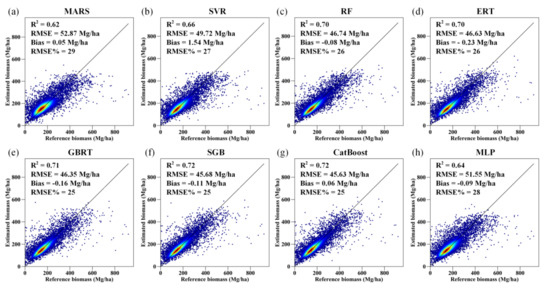
Figure 7.
Density scatter plot of the predicted AGB results obtained by the MARS, SVR, RF, ERT, GBRT, SGB, CatBoost, and MLP models (a–h) for 50 runs under the random sampling scenario.
The comparison results obtained by the different AGB modeling algorithms were consistent under the three designed scenarios. For simplicity purposes, the following results were based on the random sampling scenario.
Among the five tree-based ensemble algorithms, the CatBoost algorithm provided the most accurate estimates of forest AGB, with an R-squared of 0.71, an RMSE of 46.73 Mg/ha, a bias of 0.10 Mg/ha, and a relative RMSE of 26% (Figure S3). When the predicted AGB values corresponding to the same test samples were aggregated for each algorithm, the CatBoost model remained the best estimator and had R2, RMSE, bias, and RMSE% values of 0.72, 45.63 Mg/ha, 0.06 Mg/ha, and 25%, respectively (Figure 7). SGB had a similar accuracy to that of the CatBoost algorithm.
Despite the good performances of several algorithms for AGB estimation in terms of R2, RMSE, bias, and relative RMSE, the prediction errors induced by all the modeling algorithms were negatively correlated with the reference AGB values, indicating the overestimation of forest AGB at low values and underestimation of AGB at high values (Figure 8). The aggregation of the predictions slightly increased the correlation coefficients between the prediction error and reference AGB by approximately 0.04 for the MARS algorithm. For the other AGB modeling algorithms, the correlation coefficients remained unchanged after the aggregation.
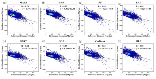
Figure 8.
Residual analysis of different modeling results obtained by the MARS, SVR, RF, ERT, GBRT, SGB, CatBoost, and MLP algorithms (a–h) under the random sampling scenario without stratification of forest types.
The problems of overestimation and underestimation were more evident for the RF, ERT, SGB, and CatBoost algorithms, with correlation coefficients of 0.84 without aggregation (Figure S4). Due to the aggregation, the boosting algorithms, SGB, and CatBoost, had correlation coefficients of 0.85 (Figure 8).
The predicted errors varied with the AGB values (Figure 9). All the models tended to overestimate forest AGB, particularly when the biomass was lower than 120 Mg/ha, and they tended to underestimate forest AGB when the biomass was higher than 210 Mg/ha. Among the eight machine learning regression algorithms, the RF, ERT, MARS, SVR, and MLP algorithms produced the most serious underestimations and overestimations of forest AGB, while the three boosting algorithms, CatBoost, GBRT, and SGB, provided less biased AGB estimates. This phenomenon could be explained by the fact that the boosting algorithms were originally designed to reduce the biases of estimators and thus provided relatively better results than those of the other algorithms in terms of bias.
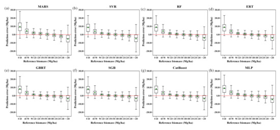
Figure 9.
Residual analysis of different modeling results obtained by the MARS, SVR, RF, ERT, GBRT, SGB, CatBoost, and MLP algorithms (a–h), along with the reference AGB ranges, under the random sampling scenario.
In summary, the CatBoost algorithm was the most suitable for AGB estimation from multiple satellite data products in terms of performance metrics, feature importance values, and overestimation and underestimation problems. SGB also provided a similar accuracy to that of the CatBoost algorithm. The RF and ERT models were slightly inferior to CatBoost and SGB models for forest AGB estimation. However, it should be noted that fewer hyperparameters need to be adjusted for the RF and ERT models than for other models, which makes them more efficient than the CatBoost and SGB algorithms.
5. Discussion
This study compared the performances of eight machine learning regression algorithms for estimating forest AGB from multiple satellite data products and ancillary information. The results showed that the five tree-base ensemble algorithms, including the RF, ERT, GBRT, SGB, and CatBoost algorithms, had similar accuracies in terms of their estimated AGB and performed better than the remaining three algorithms. The results indicated that the ensemble algorithms could improve the accuracy of estimation, which is consistent with some published studies [102,103]. In this study, the base learner of the ensemble algorithms was the regression tree model, and thus, the ensemble was homogeneous. Since the diversity of the base learners has a great effect on the performance of an ensemble algorithm, heterogeneous ensemble algorithms (e.g., stacking) that integrate different base learners could further improve the accuracy of estimated AGB, and this technique will be considered in future studies [104,105,106].
Among the eight regression algorithms, the RF and SVR models have often been used for forest AGB estimation, and their good performances have been demonstrated in published studies [7,24,107,108,109,110]. In this study, some recently developed algorithms and even some algorithms yet to be established for AGB prediction (e.g., the CatBoost and ERT algorithms), were evaluated. Comparison results showed that the CatBoost algorithm outperformed the other algorithms, including the RF and SVR models, and that the SGB also achieved good performances for forest AGB prediction. In terms of feature importance, the ERT and CatBoost algorithms provided stable results. The comparison results suggest that the recently developed algorithms performed well, and their use should be encouraged when estimating land surface parameters from remote sensing data in future studies [19]. However, it should be noted that the processes of optimizing the hyperparameters of each algorithm and comparing different algorithms to choose the best one was time consuming. Since model ensembles are becoming widespread and are improving the accuracies of estimates in many fields, integrating an AGB model with different hyperparameter configurations or integrating multiple AGB models instead of using a model selection procedure should be fully considered in future studies [111,112].
The CatBoost algorithm had good performances for AGB estimation, and could be further employed for generating the global forest biomass map since the reference AGB was collected globally in this study. Validation results showed that estimated forest AGB using the CatBoost algorithm had an accuracy with the R2 of 0.72, RMSE of 45.63Mg/ha, and relative RMSE of 25%. In another study, a global forest biomass map was generated by integrating gridded biomass datasets with the error removal and simple averaging algorithm. Cross-validation using reference AGB data showed that the accuracy of the fused global forest AGB map had an R2 of 0.61, a RMSE of 53.68 Mg/ha, and a relative RMSE of 30.28% [71]. Hu et al. [8] used RF to estimate forest biomass from GLAS data, optical imagery, climate data, and topographic data on a global scale. The R2 and RMSE between their predicted results and the validation plots were 0.56 and 87.53 Mg/ha, respectively. Yang et al. [23] used the GBRT algorithm to generate a global forest AGB map for 2005, which had the accuracy with an R2 value of 0.90 and a RMSE of 35.87 Mg/ha. The validation result was somehow overoptimistic because some of the reference data were compiled from satellite-derived biomass datasets with spatial resolutions of 500 m and 1 km. Previous studies suggested that a global forest biomass map provided by Yang et al. [23] was close to that from Hu et al. [8], when validated with field reference AGB or evaluated in terms of spatial distribution [11,71]. Therefore, compared with previous studies, this study provided a feasible way to produce accurate forest AGB maps on a global scale.
Additionally, our study highlighted that the prediction errors induced by the eight regression algorithms had strong negative correlations with forest AGB, suggesting the overestimation of AGB at low AGB values and the underestimation of forest AGB at high AGB values. Gao et al. [113] also noticed these overestimation and underestimation problems when they used Landsat TM (Thematic Mapper) and PALSAR (Phased Array type L-band Synthetic Aperture Radar) data to estimate AGB in subtropical forests. They found that the RF algorithm was not suitable for AGB prediction when the AGB values were less than 40 Mg/ha or greater than 160 Mg/ha. In this study, the eight algorithms provided their best estimates when AGB values ranged from 150 to 180 Mg/ha, but they significantly underestimated AGB when the values were larger than 210 Mg/ha and overestimated AGB when the AGB values were less than 120 Mg/ha. Zhao et al. [114] examined the data saturation problem in Landsat imagery for different vegetation types and found that the most accurate results were obtained when the AGB was 80–120 Mg/ha. In relatively low AGB (less than 40 Mg/ha) regions and high AGB (greater than 140 Mg/ha) regions, the problems of overestimation and underestimation were evident. Compared with these published studies, we observed higher saturation values of 210 Mg/ha, which could be partly attributed to the datasets used in this study. The canopy height map was originally derived from the GLAS data, which did not have the low saturation values typically found in optical and radar data for the retrieval of land surface parameters; thus, highly saturated AGB values were found. To improve the accuracy of AGB estimation, more attention should be paid to the AGB estimates at high and low values, and using data from different sources as well multistage modeling might improve the AGB estimation or mapping in the future [115,116,117].
A total of 13 predictor variables, including LAI, interannual variation in LAI, canopy height, NPP, interannual variation in NPP, tree cover, standard deviation of tree cover within each 0.01° grid, DEM, slope, temperature, changes in temperature, precipitation, and changes in precipitation, were used in all the models. Although feature importance results suggested that some variables (e.g., LAI and slope) were not quite relevant to forest AGB in the majority of models, they were not excluded in this study, since published studies have indicated the underlying mechanisms of using these variables for estimating forest AGB from remotely sensed data, and their contribution to forest AGB estimation, particularly at lower AGB values [11].
Previous studies suggested that the stratification of forest types could marginally or significantly improve the accuracy of AGB estimates [118]. However, the stratified sampling scenario did not provide more accurate estimates of forest AGB than the random sampling scenario without stratification of forest types in this study. One possible reason for this was that the choice of the stratification variable was valuable for improving AGB estimates, while the forest type was not the proper variable [119]. Additionally, modeling AGB for each forest type separately did not improve the accuracy of the estimates either, indicating that the consideration of the effects of different forest types was not straightforward for accurate AGB estimation. However, it should be noted that although modeling AGB for each forest type separately did not significantly improve the AGB estimates, it provided stable results in terms of the contributions of the predictor variables to the AGB estimates; this could help us understand the relative importance of variables in forest AGB estimation and the mechanisms of AGB dynamics in the future [120].
6. Conclusions
In this study, we evaluated eight machine learning regression algorithms for estimating forest AGB from multiple satellite data products and ancillary information. The results showed that forest AGB estimated with the tree-based ensemble algorithms, including the RF, ERT, GBRT, SGB, and CatBoost algorithms, had the mean R2 for 50 runs ranging from 0.69 to 0.71, RMSE ranging from 46.67 to 47.95 Mg/ha, bias ranging from −0.21 to 0.10 Mg/ha, and relative RMSE ranging from 26.00 to 26.72%, and were more accurate than those estimated with the MARS, SVR, and MLP algorithms with the mean R2 ranging from 0.56 to 0.66, RMSE ranging from 50.34 M to 56.69 Mg/ha, bias ranging from −0.02 to 1.55 Mg/ha, and relative RMSE ranging from 28.05 to 31.58%. Both the stratification of forest types and the modeling of AGB for each forest type separately for the eight machine learning algorithms did not result in more accurate AGB estimates than those obtained under the random sampling scenario. All eight AGB modeling algorithms underestimated forest AGB when the AGB values were larger than 210 Mg/ha and overestimated forest AGB when the values were less than 120 Mg/ha. Further efforts should be made to improve the AGB estimates at low and high AGB values.
Among the eight algorithms, the CatBoost model exhibited the best performance with an R2 of 0.72, an RMSE of 45.63 Mg/ha, a bias of 0.06 Mg/ha, and a relative RMSE of 25% when predicted AGB values for 50 runs were aggregated, and it also provided stable results in terms of the feature importance of the predictor variables. Furthermore, it resulted in less serious underestimation and overestimation of AGB than the other models under the three scenarios. Therefore, the CatBoost algorithm is recommended for AGB estimation from multi-satellite data.
However, it should be noted that the processes of hyperparameter optimization for each algorithm and model comparison for selecting the best one was time consuming. In future studies, ensemble methods that integrate versions of an algorithm with different hyperparameter configurations or include diverse algorithms instead of using a model selection procedure will be considered for further improving the AGB estimates.
Supplementary Materials
The following are available online at https://www.mdpi.com/2072-4292/12/24/4015/s1, Figure S1: feature importance values for the predictor variables in the eight machine learning regression algorithms under the stratified sampling scenario, Figure S2: feature importance values for the predictor variables in the eight machine learning regression algorithms under the separate modeling scenario, Figure S3: density scatter plot of the predicted AGB values generated by simply combining the results of the MARS, SVR, RF, ERT, GBRT, SGB, CatBoost, and MLP algorithms for 50 runs under the random sampling scenario, Figure S4: residual analysis of the different modeling results that were obtained by simply combining the predictions of the MARS, SVR, RF, ERT, GBRT, SGB, CatBoost, and MLP algorithms for 50 runs under the random sampling scenario.
Author Contributions
Y.Z. conceived the study; Y.Z. and J.M. performed the data analysis; Y.Z., J.M., S.L., X.L., and M.L. contributed to writing the manuscript. All authors have read and agreed to the published version of the manuscript.
Funding
This work was supported by the National Key Research and Development Program of China (2018YFC1407103 and 2016YFA0600103), the National Natural Science Foundation of China (Grant No. 41801347), and the Fundamental Research Funds for the Central Universities (No. FRF-TP-19-041A2).
Conflicts of Interest
The authors declare no conflict of interest.
References
- Sessa, R. Assessment of the status of the development of the standards for the terrestrial essential climate variables: Biomass. Gto Syst. Rome Italy Version 2009, 10, 1–18. [Google Scholar]
- Hall, F.G.; Bergen, K.; Blair, J.B.; Dubayah, R.; Houghton, R.; Hurtt, G.; Kellndorfer, J.; Lefsky, M.; Ranson, J.; Saatchi, S.; et al. Characterizing 3D vegetation structure from space: Mission requirements. Remote Sens. Environ. 2011, 115, 2753–2775. [Google Scholar] [CrossRef]
- Le Toan, T.; Quegan, S.; Davidson, M.W.J.; Balzter, H.; Paillou, P.; Papathanassiou, K.; Plummer, S.; Rocca, F.; Saatchi, S.; Shugart, H.; et al. The BIOMASS mission: Mapping global forest biomass to better understand the terrestrial carbon cycle. Remote Sens. Environ. 2011, 115, 2850–2860. [Google Scholar] [CrossRef]
- Zolkos, S.G.; Goetz, S.J.; Dubayah, R. A meta-analysis of terrestrial aboveground biomass estimation using lidar remote sensing. Remote Sens. Environ. 2013, 128, 289–298. [Google Scholar] [CrossRef]
- Saatchi, S.S.; Harris, N.L.; Brown, S.; Lefsky, M.; Mitchard, E.T.A.; Salas, W.; Zutta, B.R.; Buermann, W.; Lewis, S.L.; Hagen, S.; et al. Benchmark map of forest carbon stocks in tropical regions across three continents. Proc. Natl. Acad. Sci. USA 2011, 108, 9899–9904. [Google Scholar] [CrossRef] [PubMed]
- Baccini, A.; Goetz, S.J.; Walker, W.S.; Laporte, N.T.; Sun, M.; Sulla-Menashe, D.; Hackler, J.; Beck, P.S.A.; Dubayah, R.; Friedl, M.A.; et al. Estimated carbon dioxide emissions from tropical deforestation improved by carbon-density maps. Nat. Clim. Chang. 2012, 2, 182–185. [Google Scholar] [CrossRef]
- Cartus, O.; Kellndorfer, J.; Walker, W.; Franco, C.; Bishop, J.; Santos, L.; Fuentes, J. A National, Detailed Map of Forest Aboveground Carbon Stocks in Mexico. Remote Sens. 2014, 6, 5559–5588. [Google Scholar] [CrossRef]
- Hu, T.; Su, Y.; Xue, B.; Liu, J.; Zhao, X.; Fang, J.; Guo, Q. Mapping Global Forest Aboveground Biomass with Spaceborne LiDAR, Optical Imagery, and Forest Inventory Data. Remote Sens. 2016, 8, 565. [Google Scholar] [CrossRef]
- Eggleston, H.; Buendia, L.; Miwa, K.; Ngara, T.; Tanabe, K. IPCC Guidelines for National Greenhouse Gas Inventories; Institute for Global Environmental Strategies: Hayama, Japan, 2006. [Google Scholar]
- Qi, Y.; Wei, W.; Chen, C.; Chen, L. Plant root-shoot biomass allocation over diverse biomes: A global synthesis. Glob. Ecol. Conserv. 2019, 18, e00606. [Google Scholar] [CrossRef]
- Zhang, Y.; Liang, S.; Yang, L. A Review of Regional and Global Gridded Forest Biomass Datasets. Remote Sens. 2019, 11, 2744. [Google Scholar] [CrossRef]
- Lu, D.; Chen, Q.; Wang, G.; Moran, E.; Batistella, M.; Zhang, M.; Vaglio Laurin, G.; Saah, D. Aboveground Forest Biomass Estimation with Landsat and LiDAR Data and Uncertainty Analysis of the Estimates. Int. J. Res. 2012, 2012, 16. [Google Scholar] [CrossRef]
- Mitchard, E.T.A.; Feldpausch, T.R.; Brienen, R.J.W.; Lopez-Gonzalez, G.; Monteagudo, A.; Baker, T.R.; Lewis, S.L.; Lloyd, J.; Quesada, C.A.; Gloor, M.; et al. Markedly divergent estimates of Amazon forest carbon density from ground plots and satellites. Glob. Ecol. Biogeogr. 2014, 23, 935–946. [Google Scholar] [CrossRef] [PubMed]
- Lu, D. The potential and challenge of remote sensing-based biomass estimation. Int. J. Remote Sens. 2006, 27, 1297–1328. [Google Scholar] [CrossRef]
- Navarro, J.A.; Algeet, N.; Fernández-Landa, A.; Esteban, J.; Rodríguez-Noriega, P.; Guillén-Climent, M.L. Integration of UAV, Sentinel-1, and Sentinel-2 Data for Mangrove Plantation Aboveground Biomass Monitoring in Senegal. Remote Sens. 2019, 11, 77. [Google Scholar] [CrossRef]
- Vafaei, S.; Soosani, J.; Adeli, K.; Fadaei, H.; Naghavi, H.; Pham, T.D.; Tien Bui, D. Improving Accuracy Estimation of Forest Aboveground Biomass Based on Incorporation of ALOS-2 PALSAR-2 and Sentinel-2A Imagery and Machine Learning: A Case Study of the Hyrcanian Forest Area (Iran). Remote Sens. 2018, 10, 172. [Google Scholar] [CrossRef]
- Domingues, G.F.; Soares, V.P.; Leite, H.G.; Ferraz, A.S.; Ribeiro, C.A.A.S.; Lorenzon, A.S.; Marcatti, G.E.; Teixeira, T.R.; de Castro, N.L.M.; Mota, P.H.S.; et al. Artificial neural networks on integrated multispectral and SAR data for high-performance prediction of eucalyptus biomass. Comput. Electron. Agric. 2020, 168, 105089. [Google Scholar] [CrossRef]
- Li, Y.; Li, C.; Li, M.; Liu, Z. Influence of Variable Selection and Forest Type on Forest Aboveground Biomass Estimation Using Machine Learning Algorithms. Forests 2019, 10, 1073. [Google Scholar] [CrossRef]
- Reichstein, M.; Camps-Valls, G.; Stevens, B.; Jung, M.; Denzler, J.; Carvalhais, N.; Prabhat. Deep learning and process understanding for data-driven Earth system science. Nature 2019, 566, 195–204. [Google Scholar] [CrossRef]
- Breiman, L.; Friedman, J.; Stone, C.J.; Olshen, R.A. Classification and Regression Trees; CRC Press: Boca Raton, FL, USA, 1984. [Google Scholar]
- Zhang, Y.; Liang, S.; Sun, G. Forest biomass mapping of Northeastern China Using GLAS and MODIS Data. IEEE J. Sel. Top. Appl. Earth Obs. Remote Sens. 2014, 7, 140–152. [Google Scholar] [CrossRef]
- Su, Y.; Guo, Q.; Xue, B.; Hu, T.; Alvarez, O.; Tao, S.; Fang, J. Spatial distribution of forest aboveground biomass in China: Estimation through combination of spaceborne lidar, optical imagery, and forest inventory data. Remote Sens. Environ. 2016, 173, 187–199. [Google Scholar] [CrossRef]
- Yang, L.; Liang, S.; Zhang, Y. A New Method for Generating a Global Forest Aboveground Biomass Map From Multiple High-Level Satellite Products and Ancillary Information. IEEE J. Sel. Top. Appl. Earth Obs. Remote Sens. 2020, 13, 2587–2597. [Google Scholar] [CrossRef]
- Almeida, C.T.d.; Galvão, L.S.; Aragão, L.E.d.O.C.e.; Ometto, J.P.H.B.; Jacon, A.D.; Pereira, F.R.d.S.; Sato, L.Y.; Lopes, A.P.; Graça, P.M.L.d.A.; Silva, C.V.d.J.; et al. Combining LiDAR and hyperspectral data for aboveground biomass modeling in the Brazilian Amazon using different regression algorithms. Remote Sens. Environ. 2019, 232, 111323. [Google Scholar] [CrossRef]
- Gleason, C.J.; Im, J. Forest biomass estimation from airborne LiDAR data using machine learning approaches. Remote Sens. Environ. 2012, 125, 80–91. [Google Scholar] [CrossRef]
- Beaudoin, A.; Bernier, P.Y.; Guindon, L.; Villemaire, P.; Guo, X.J.; Stinson, G.; Bergeron, T.; Magnussen, S.; Hall, R.J. Mapping attributes of Canada’s forests at moderate resolution through kNN and MODIS imagery. Can. J. Res. 2014, 44, 521–532. [Google Scholar] [CrossRef]
- Güneralp, İ.; Filippi, A.M.; Randall, J. Estimation of floodplain aboveground biomass using multispectral remote sensing and nonparametric modeling. Int. J. Appl. Earth. Obs. Geoinf. 2014, 33, 119–126. [Google Scholar] [CrossRef]
- López-Serrano, P.M.; Corral-Rivas, J.J.; Díaz-Varela, R.A.; Álvarez-González, J.G.; López-Sánchez, C.A. Evaluation of Radiometric and Atmospheric Correction Algorithms for Aboveground Forest Biomass Estimation Using Landsat 5 TM Data. Remote Sens. 2016, 8, 369. [Google Scholar] [CrossRef]
- Wu, C.; Shen, H.; Shen, A.; Deng, J.; Gan, M.; Zhu, J.; Xu, H.; Wang, K. Comparison of machine-learning methods for above-ground biomass estimation based on Landsat imagery. J. Appl. Remote. Sens. 2016, 10, 035010. [Google Scholar] [CrossRef]
- Pham, T.D.; Yokoya, N.; Xia, J.; Ha, N.T.; Le, N.N.; Nguyen, T.T.T.; Dao, T.H.; Vu, T.T.P.; Pham, T.D.; Takeuchi, W. Comparison of Machine Learning Methods for Estimating Mangrove Above-Ground Biomass Using Multiple Source Remote Sensing Data in the Red River Delta Biosphere Reserve, Vietnam. Remote Sens. 2020, 12, 1334. [Google Scholar] [CrossRef]
- Shang, K.; Yao, Y.; Li, Y.; Yang, J.; Jia, K.; Zhang, X.; Chen, X.; Bei, X.; Guo, X. Fusion of Five Satellite-Derived Products Using Extremely Randomized Trees to Estimate Terrestrial Latent Heat Flux over Europe. Remote Sens. 2020, 12, 687. [Google Scholar] [CrossRef]
- Wei, J.; Li, Z.Q.; Cribb, M.; Huang, W.; Xue, W.H.; Sun, L.; Guo, J.P.; Peng, Y.R.; Li, J.; Lyapustin, A.; et al. Improved 1 km resolution PM2.5 estimates across China using enhanced space-time extremely randomized trees. Atmos. Chem. Phys. 2020, 20, 3273–3289. [Google Scholar] [CrossRef]
- Feng, Y.; Lu, D.; Chen, Q.; Keller, M.; Moran, E.; dos-Santos, M.N.; Bolfe, E.L.; Batistella, M. Examining effective use of data sources and modeling algorithms for improving biomass estimation in a moist tropical forest of the Brazilian Amazon. Int. J. Digit Earth. 2017, 10, 996–1016. [Google Scholar] [CrossRef]
- Fayad, I.; Baghdadi, N.; Bailly, J.-S.; Barbier, N.; Gond, V.; Hajj, M.E.; Fabre, F.; Bourgine, B. Canopy Height Estimation in French Guiana with LiDAR ICESat/GLAS Data Using Principal Component Analysis and Random Forest Regressions. Remote Sens. 2014, 6, 11883–11914. [Google Scholar] [CrossRef]
- Vaglio Laurin, G.; Puletti, N.; Chen, Q.; Corona, P.; Papale, D.; Valentini, R. Above ground biomass and tree species richness estimation with airborne lidar in tropical Ghana forests. Int. J. Appl. Earth. Obs. Geoinf. 2016, 52, 371–379. [Google Scholar] [CrossRef]
- Friedman, J.H. Multivariate Adaptive Regression Splines. Ann. Stat. 1991, 19, 1–67. [Google Scholar] [CrossRef]
- Halme, E.; Pellikka, P.; Mõttus, M. Utility of hyperspectral compared to multispectral remote sensing data in estimating forest biomass and structure variables in Finnish boreal forest. Int. J. Appl. Earth. Obs. Geoinf. 2019, 83, 101942. [Google Scholar] [CrossRef]
- Mountrakis, G.; Im, J.; Ogole, C. Support vector machines in remote sensing: A review. ISPRS J. Photogramm. Remote Sens. 2011, 66, 247–259. [Google Scholar] [CrossRef]
- Liu, K.; Wang, J.; Zeng, W.; Song, J. Comparison and Evaluation of Three Methods for Estimating Forest above Ground Biomass Using TM and GLAS Data. Remote Sens. 2017, 9, 341. [Google Scholar] [CrossRef]
- Schulz, E.; Speekenbrink, M.; Krause, A. A tutorial on Gaussian process regression: Modelling, exploring, and exploiting functions. J. Math. Psychol. 2018, 85, 1–16. [Google Scholar] [CrossRef]
- Verrelst, J.; Muñoz, J.; Alonso, L.; Delegido, J.; Rivera, J.P.; Camps-Valls, G.; Moreno, J. Machine learning regression algorithms for biophysical parameter retrieval: Opportunities for Sentinel-2 and -3. Remote Sens. Environ. 2012, 118, 127–139. [Google Scholar] [CrossRef]
- Blackard, J.A.; Finco, M.V.; Helmer, E.H.; Holden, G.R.; Hoppus, M.L.; Jacobs, D.M.; Lister, A.J.; Moisen, G.G.; Nelson, M.D.; Riemann, R.; et al. Mapping U.S. forest biomass using nationwide forest inventory data and moderate resolution information. Remote Sens. Environ. 2008, 112, 1658–1677. [Google Scholar] [CrossRef]
- Dietterich, T.G. An Experimental Comparison of Three Methods for Constructing Ensembles of Decision Trees: Bagging, Boosting, and Randomization. Mach. Learn. 2000, 40, 139–157. [Google Scholar] [CrossRef]
- Erdal, H.I.; Karakurt, O. Advancing monthly streamflow prediction accuracy of CART models using ensemble learning paradigms. J. Hydrol. 2013, 477, 119–128. [Google Scholar] [CrossRef]
- Lin, N.; Noe, D.; He, X. Tree-Based Methods and Their Applications. In Springer Handbook of Engineering Statistics; Pham, H., Ed.; Springer: London, UK, 2006; pp. 551–570. [Google Scholar] [CrossRef]
- Zhao, Q.; Yu, S.; Zhao, F.; Tian, L.; Zhao, Z. Comparison of machine learning algorithms for forest parameter estimations and application for forest quality assessments. Ecol. Manag. 2019, 434, 224–234. [Google Scholar] [CrossRef]
- Yang, P.; Yang, Y.H.; Zhou, B.B.; Zomaya, A.Y. A Review of Ensemble Methods in Bioinformatics. Curr. Bioinform. 2010, 5, 296–308. [Google Scholar] [CrossRef]
- Geurts, P.; Ernst, D.; Wehenkel, L. Extremely randomized trees. Mach. Learn. 2006, 63, 3–42. [Google Scholar] [CrossRef]
- Breiman, L. Random Forests. Mach. Learn. 2001, 45, 5–32. [Google Scholar] [CrossRef]
- Geurts, P.; Louppe, G. Learning to Rank with Extremely Randomized Trees. In Proceedings of the Learning to Rank Challenge, Machine Learning Research. 2011, pp. 49–61. Available online: http://proceedings.mlr.press/v14/geurts11a/geurts11a.pdf (accessed on 24 June 2020).
- Eslami, E.; Salman, A.K.; Choi, Y.; Sayeed, A.; Lops, Y. A data ensemble approach for real-time air quality forecasting using extremely randomized trees and deep neural networks. Neural. Comput. Appl. 2020, 32, 7563–7579. [Google Scholar] [CrossRef]
- Galelli, S.; Castelletti, A. Assessing the predictive capability of randomized tree-based ensembles in streamflow modelling. Hydrol. Earth Syst. Sci. 2013, 17, 2669–2684. [Google Scholar] [CrossRef]
- Buhlmann, P.; Hothorn, T. Boosting Algorithms: Regularization, Prediction and Model Fitting. Stat. Sci. 2007, 22, 477–505. [Google Scholar] [CrossRef]
- Friedman, J.H. Greedy function approximation: A gradient boosting machine. Ann. Stat. 2001, 29, 1189–1232. [Google Scholar] [CrossRef]
- Friedman, J.H. Stochastic gradient boosting. Comput. Stat. Data Anal. 2002, 38, 367–378. [Google Scholar] [CrossRef]
- Moisen, G.G.; Freeman, E.A.; Blackard, J.A.; Frescino, T.S.; Zimmermann, N.E.; Edwards, T.C. Predicting tree species presence and basal area in Utah: A comparison of stochastic gradient boosting, generalized additive models, and tree-based methods. Ecol. Model. 2006, 199, 176–187. [Google Scholar] [CrossRef]
- Filippi, A.M.; Güneralp, İ.; Randall, J. Hyperspectral remote sensing of aboveground biomass on a river meander bend using multivariate adaptive regression splines and stochastic gradient boosting. Remote Sens. Lett. 2014, 5, 432–441. [Google Scholar] [CrossRef]
- Prokhorenkova, L.; Gusev, G.; Vorobev, A.; Dorogush, A.V.; Gulin, A. CatBoost: Unbiased boosting with categorical features. In Advances in Neural Information Processing Systems 31; Bengio, S., Wallach, H., Larochelle, H., Grauman, K., CesaBianchi, N., Garnett, R., Eds.; Curran Associates Inc.: Red Hook, NY, USA, 2018; Volume 31. [Google Scholar]
- Dev, V.A.; Eden, M.R. Formation lithology classification using scalable gradient boosted decision trees. Comput. Chem Eng. 2019, 128, 392–404. [Google Scholar] [CrossRef]
- Huang, G.; Wu, L.; Ma, X.; Zhang, W.; Fan, J.; Yu, X.; Zeng, W.; Zhou, H. Evaluation of CatBoost method for prediction of reference evapotranspiration in humid regions. J. Hydrol. 2019, 574, 1029–1041. [Google Scholar] [CrossRef]
- Jiang, Y.; Yang, C.; Na, J.; Li, G.; Li, Y.; Zhong, J. A Brief Review of Neural Networks Based Learning and Control and Their Applications for Robots. Complexity 2017, 2017, 1895897. [Google Scholar] [CrossRef]
- Foody, G.M.; Cutler, M.E.; McMorrow, J.; Pelz, D.; Tangki, H.; Boyd, D.S.; Douglas, I. Mapping the biomass of Bornean tropical rain forest from remotely sensed data. Glob. Ecol. Biogeogr. 2001, 10, 379–387. [Google Scholar] [CrossRef]
- Ozcelik, R.; Diamantopoulou, M.J.; Eker, M.; Gurlevik, N. Artificial Neural Network Models: An Alternative Approach for Reliable Aboveground Pine Tree Biomass Prediction. Science 2017, 63, 291–302. [Google Scholar] [CrossRef]
- Nandy, S.; Singh, R.; Ghosh, S.; Watham, T.; Kushwaha, S.P.S.; Kumar, A.S.; Dadhwal, V.K. Neural network-based modelling for forest biomass assessment. Carbon Manag. 2017, 8, 305–317. [Google Scholar] [CrossRef]
- Englhart, S.; Keuck, V.; Siegert, F. Modeling Aboveground Biomass in Tropical Forests Using Multi-Frequency SAR Data—A Comparison of Methods. IEEE J. Sel. Top. Appl. Earth Obs. Remote Sens. 2012, 5, 298–306. [Google Scholar] [CrossRef]
- Sovilj, D.; Eirola, E.; Miche, Y.; Björk, K.-M.; Nian, R.; Akusok, A.; Lendasse, A. Extreme learning machine for missing data using multiple imputations. Neurocomputing 2016, 174, 220–231. [Google Scholar] [CrossRef]
- Huang, G.; Huang, G.-B.; Song, S.; You, K. Trends in extreme learning machines: A review. Neural Netw. (USA) 2015, 61, 32–48. [Google Scholar] [CrossRef] [PubMed]
- Huang, G.; Zhou, H.; Ding, X.; Zhang, R. Extreme Learning Machine for Regression and Multiclass Classification. IEEE Trans. Syst. Man Cybern. Syst. Part B (Cybern.) 2012, 42, 513–529. [Google Scholar] [CrossRef] [PubMed]
- Ding, S.; Zhao, H.; Zhang, Y.; Xu, X.; Nie, R. Extreme learning machine: Algorithm, theory and applications. Artif. Intell. Rev. 2015, 44, 103–115. [Google Scholar] [CrossRef]
- Duncanson, L.; Armston, J.; Disney, M.; Avitabile, V.; Barbier, N.; Calders, K.; Carter, S.; Chave, J.; Herold, M.; Crowther, T.W.; et al. The Importance of Consistent Global Forest Aboveground Biomass Product Validation. Surv. Geophys. 2019, 40, 979–999. [Google Scholar] [CrossRef]
- Zhang, Y.; Liang, S. Fusion of Multiple Gridded Biomass Datasets for Generating a Global Forest Aboveground Biomass Map. Remote Sens. 2020, 12, 2559. [Google Scholar] [CrossRef]
- Sulla-Menashe, D.; Gray, J.M.; Abercrombie, S.P.; Friedl, M.A. Hierarchical mapping of annual global land cover 2001 to present: The MODIS Collection 6 Land Cover product. Remote Sens. Environ. 2019, 222, 183–194. [Google Scholar] [CrossRef]
- Hyde, P.; Nelson, R.; Kimes, D.; Levine, E. Exploring LiDAR–RaDAR synergy—Predicting aboveground biomass in a southwestern ponderosa pine forest using LiDAR, SAR and InSAR. Remote Sens. Environ. 2007, 106, 28–38. [Google Scholar] [CrossRef]
- Sun, G.; Ranson, K.J.; Guo, Z.; Zhang, Z.; Montesano, P.; Kimes, D. Forest biomass mapping from lidar and radar synergies. Remote Sens. Environ. 2011, 115, 2906–2916. [Google Scholar] [CrossRef]
- Tsui, O.W.; Coops, N.C.; Wulder, M.A.; Marshall, P.L. Integrating airborne LiDAR and space-borne radar via multivariate kriging to estimate above-ground biomass. Remote Sens. Environ. 2013, 139, 340–352. [Google Scholar] [CrossRef]
- Shao, Z.; Zhang, L.; Wang, L. Stacked Sparse Autoencoder Modeling Using the Synergy of Airborne LiDAR and Satellite Optical and SAR Data to Map Forest Above-Ground Biomass. IEEE J. Sel. Top. Appl. Earth Obs. Remote Sens. 2017, 10, 5569–5582. [Google Scholar] [CrossRef]
- Zhang, G.; Ganguly, S.; Nemani, R.R.; White, M.A.; Milesi, C.; Hashimoto, H.; Wang, W.; Saatchi, S.; Yu, Y.; Myneni, R.B. Estimation of forest aboveground biomass in California using canopy height and leaf area index estimated from satellite data. Remote Sens. Environ. 2014, 151, 44–56. [Google Scholar] [CrossRef]
- Keeling, H.C.; Phillips, O.L. The global relationship between forest productivity and biomass. Glob. Ecol. Biogeogr. 2007, 16, 618–631. [Google Scholar] [CrossRef]
- Sadeghi, Y.; St-Onge, B.; Leblon, B.; Prieur, J.F.; Simard, M. Mapping boreal forest biomass from a SRTM and TanDEM-X based on canopy height model and Landsat spectral indices. Int. J. Appl. Earth. Obs. Geoinf. 2018, 68, 202–213. [Google Scholar] [CrossRef]
- Chen, L.; Wang, Y.; Ren, C.; Zhang, B.; Wang, Z. Optimal Combination of Predictors and Algorithms for Forest Above-Ground Biomass Mapping from Sentinel and SRTM Data. Remote Sens. 2019, 11, 414. [Google Scholar] [CrossRef]
- Simard, M.; Rivera-Monroy, V.H.; Mancera-Pineda, J.E.; Castaneda-Moya, E.; Twilley, R.R. A systematic method for 3D mapping of mangrove forests based on Shuttle Radar Topography Mission elevation data, ICEsat/GLAS waveforms and field data: Application to Cienaga Grande de Santa Marta, Colombia. Remote Sens. Environ. 2008, 112, 2131–2144. [Google Scholar] [CrossRef]
- Fatoyinbo, T.E.; Simard, M. Height and biomass of mangroves in Africa from ICESat/GLAS and SRTM. Int. J. Remote Sens. 2013, 34, 668–681. [Google Scholar] [CrossRef]
- Fayad, I.; Baghdadi, N.; Gond, V.; Bailly, J.S.; Barbier, N.; El Hajj, M.; Fabre, F. Coupling potential of ICESat/GLAS and SRTM for the discrimination of forest landscape types in French Guiana. Int. J. Appl. Earth. Obs. Geoinf. 2014, 33, 21–31. [Google Scholar] [CrossRef]
- Liang, S.; Cheng, J.; Jia, K.; Jiang, B.; Liu, Q.; Xiao, Z.; Yao, Y.; Yuan, W.; Zhang, X.; Zhao, X.; et al. The Global LAnd Surface Satellite (GLASS) product suite. Bull. Am. Meteorol. Soc. 2020, 1–37. [Google Scholar] [CrossRef]
- Li, X.L.; Lu, H.; Yu, L.; Yang, K. Comparison of the Spatial Characteristics of Four Remotely Sensed Leaf Area Index Products over China: Direct Validation and Relative Uncertainties. Remote Sens. 2018, 10, 148. [Google Scholar] [CrossRef]
- Xiao, Z.; Liang, S.; Wang, J.; Chen, P.; Yin, X.; Zhang, L.; Song, J. Use of General Regression Neural Networks for Generating the GLASS Leaf Area Index Product From Time-Series MODIS Surface Reflectance. IEEE Trans. Geosci. Remote Sens. 2014, 52, 209–223. [Google Scholar] [CrossRef]
- Xiao, Z.; Liang, S.; Wang, J.; Xiang, Y.; Zhao, X.; Song, J. Long-Time-Series Global Land Surface Satellite Leaf Area Index Product Derived From MODIS and AVHRR Surface Reflectance. IEEE Trans. Geosci. Remote Sens. 2016, 54, 5301–5318. [Google Scholar] [CrossRef]
- Simard, M.; Pinto, N.; Fisher, J.B.; Baccini, A. Mapping forest canopy height globally with spaceborne lidar. J. Geophys. Res. Biogeosci. 2011, 116, G04021. [Google Scholar] [CrossRef]
- Lefsky, M.A. A global forest canopy height map from the Moderate Resolution Imaging Spectroradiometer and the Geoscience Laser Altimeter System. Geophys. Res. Lett. 2010, 37, L15401. [Google Scholar] [CrossRef]
- Bolton, D.K.; Coops, N.C.; Wulder, M.A. Investigating the agreement between global canopy height maps and airborne Lidar derived height estimates over Canada. Can. J. Remote. Sens. 2013, 39, S139–S151. [Google Scholar] [CrossRef]
- Gulbeyaz, O.; Bond-Lamberty, B.; Akyurek, Z.; West, T.O. A new approach to evaluate the MODIS annual NPP product (MOD17A3) using forest field data from Turkey. Int. J. Remote Sens. 2018, 39, 2560–2578. [Google Scholar] [CrossRef]
- Running, S.; Zhao, M. MOD17A3HGF MODIS/Terra Net Primary Production Gap-Filled Yearly L4 Global 500 m SIN Grid V006 NASA EOSDIS Land Processes DAAC. 2019. Available online: https://doi.org/10.5067/MODIS/MOD17A3HGF.006 (accessed on 3 May 2020).
- Hansen, M.C.; Potapov, P.V.; Moore, R.; Hancher, M.; Turubanova, S.A.; Tyukavina, A.; Thau, D.; Stehman, S.V.; Goetz, S.J.; Loveland, T.R.; et al. High-Resolution Global Maps of 21st-Century Forest Cover Change. Science 2013, 342, 850–853. [Google Scholar] [CrossRef]
- Réjou-Méchain, M.; Muller-Landau, H.C.; Detto, M.; Thomas, S.C.; Le Toan, T.; Saatchi, S.S.; Barreto-Silva, J.S.; Bourg, N.A.; Bunyavejchewin, S.; Butt, N.; et al. Local spatial structure of forest biomass and its consequences for remote sensing of carbon stocks. Biogeosciences 2014, 11, 6827–6840. [Google Scholar] [CrossRef]
- Danielson, J.J.; Gesch, D.B. Global Multi-Resolution Terrain Elevation Data 2010 (GMTED2010); 2011-1073; Earth Resources Observation and Science Center: Sioux Falls, SD, USA, 2011. [Google Scholar]
- Fick, S.E.; Hijmans, R.J. WorldClim 2: New 1-km spatial resolution climate surfaces for global land areas. Int. J. Clim. 2017, 37, 4302–4315. [Google Scholar] [CrossRef]
- Harris, I.; Jones, P.D.; Osborn, T.J.; Lister, D.H. Updated high-resolution grids of monthly climatic observations—the CRU TS3.10 Dataset. Int. J. Clim. 2014, 34, 623–642. [Google Scholar] [CrossRef]
- Pedregosa, F.; Varoquaux, G.; Gramfort, A.; Michel, V.; Thirion, B.; Grisel, O.; Blondel, M.; Prettenhofer, P.; Weiss, R.; Dubourg, V.; et al. Scikit-learn: Machine Learning in Python. J. Mach. Learn. Res. 2011, 12, 2825–2830. [Google Scholar]
- Bhadra, S.; Sagan, V.; Maimaitijiang, M.; Maimaitiyiming, M.; Newcomb, M.; Shakoor, N.; Mockler, T.C. Quantifying Leaf Chlorophyll Concentration of Sorghum from Hyperspectral Data Using Derivative Calculus and Machine Learning. Remote Sens. 2020, 12, 2082. [Google Scholar] [CrossRef]
- Attoh-Okine, N.O.; Mensah, S.; Nawaiseh, M. A new technique for using multivariate adaptive regression splines (MARS) in pavement roughness prediction. Proc. Inst. Civ. Eng. Transp. 2003, 156, 51–55. [Google Scholar] [CrossRef]
- Greenwell, B.M.; Boehmke, B.C.; McCarthy, A.J. A Simple and Effective Model-Based Variable Importance Measure. arXiv 2018, arXiv:1805.04755. [Google Scholar]
- Healey, S.P.; Cohen, W.B.; Yang, Z.; Kenneth Brewer, C.; Brooks, E.B.; Gorelick, N.; Hernandez, A.J.; Huang, C.; Joseph Hughes, M.; Kennedy, R.E.; et al. Mapping forest change using stacked generalization: An ensemble approach. Remote Sens. Environ. 2018, 204, 717–728. [Google Scholar] [CrossRef]
- Xu, M.; Liu, H.X.; Beck, R.; Lekki, J.; Yang, B.; Shu, S.; Kang, E.L.; Anderson, R.; Johansen, R.; Emery, E.; et al. A spectral space partition guided ensemble method for retrieving chlorophyll-a concentration in inland waters from Sentinel-2A satellite imagery. J. Great Lakes Res. 2019, 45, 454–465. [Google Scholar] [CrossRef]
- Tyralis, H.; Papacharalampous, G.; Burnetas, A.; Langousis, A. Hydrological post-processing using stacked generalization of quantile regression algorithms: Large-scale application over CONUS. J. Hydrol. 2019, 577. [Google Scholar] [CrossRef]
- Sesmero, M.P.; Ledezma, A.I.; Sanchis, A. Generating ensembles of heterogeneous classifiers using Stacked Generalization. Wires Data Min. Knowl. Discov. 2015, 5, 21–34. [Google Scholar] [CrossRef]
- Zouggar, S.T.; Adla, A. A Diversity-Accuracy Measure for Homogenous Ensemble Selection. Int. J. Interact. Multi. 2019, 5, 63–70. [Google Scholar] [CrossRef]
- Li, Y.; Li, M.; Li, C.; Liu, Z. Forest aboveground biomass estimation using Landsat 8 and Sentinel-1A data with machine learning algorithms. Sci. Rep. 2020, 10, 9952. [Google Scholar] [CrossRef]
- Vieilledent, G.; Gardi, O.; Grinand, C.; Burren, C.; Andriamanjato, M.; Camara, C.; Gardner, C.J.; Glass, L.; Rasolohery, A.; Ratsimba, H.R. Bioclimatic envelope models predict a decrease in tropical forest carbon stocks with climate change in Madagascar. J. Ecol. 2016, 104, 703–715. [Google Scholar] [CrossRef]
- López-Serrano, P.M.; López-Sánchez, C.A.; Álvarez-González, J.G.; García-Gutiérrez, J. A Comparison of Machine Learning Techniques Applied to Landsat-5 TM Spectral Data for Biomass Estimation. Can. J. Remote. Sens. 2016, 42, 690–705. [Google Scholar] [CrossRef]
- Liang, S.; Wang, J. Advanced Remote Sensing: Terrestrial Information Extraction and Applications; Academic Press: Cambridge, UK, 2019. [Google Scholar]
- Ren, Y.; Suganthan, P.N.; Srikanth, N. Ensemble methods for wind and solar power forecasting—A state-of-the-art review. Renew. Sust. Energ. Rev. 2015, 50, 82–91. [Google Scholar] [CrossRef]
- Yang, S.; Browne, A. Neural network ensembles: Combining multiple models for enhanced performance using a multistage approach. Expert Syst. 2004, 21, 279–288. [Google Scholar] [CrossRef]
- Gao, Y.; Lu, D.; Li, G.; Wang, G.; Chen, Q.; Liu, L.; Li, D. Comparative Analysis of Modeling Algorithms for Forest Aboveground Biomass Estimation in a Subtropical Region. Remote Sens. 2018, 10, 627. [Google Scholar] [CrossRef]
- Zhao, P.; Lu, D.; Wang, G.; Wu, C.; Huang, Y.; Yu, S. Examining Spectral Reflectance Saturation in Landsat Imagery and Corresponding Solutions to Improve Forest Aboveground Biomass Estimation. Remote Sens. 2016, 8, 469. [Google Scholar] [CrossRef]
- Yao, Y.; Gao, F. A survey on multistage/multiphase statistical modeling methods for batch processes. Annu. Rev. Control 2009, 33, 172–183. [Google Scholar] [CrossRef]
- Bouvet, A.; Mermoz, S.; Le Toan, T.; Villard, L.; Mathieu, R.; Naidoo, L.; Asner, G.P. An above-ground biomass map of African savannahs and woodlands at 25m resolution derived from ALOS PALSAR. Remote Sens. Environ. 2018, 206, 156–173. [Google Scholar] [CrossRef]
- Akhtar, A.M.; Qazi, W.A.; Ahmad, S.R.; Gilani, H.; Mahmood, S.A.; Rasool, A. Integration of high-resolution optical and SAR satellite remote sensing datasets for aboveground biomass estimation in subtropical pine forest, Pakistan. Environ. Monit. Assess. 2020, 192, 584. [Google Scholar] [CrossRef]
- Jiang, X.; Li, G.; Lu, D.; Chen, E.; Wei, X. Stratification-Based Forest Aboveground Biomass Estimation in a Subtropical Region Using Airborne Lidar Data. Remote Sens. 2020, 12, 1101. [Google Scholar] [CrossRef]
- Eskelson, B.N.I.; Temesgen, H.; Barrett, T.M. Comparison of stratified and non-stratified most similar neighbour imputation for estimating stand tables. For. Int. J. Res. 2008, 81, 125–134. [Google Scholar] [CrossRef]
- Zhang, Y.; Liang, S. Changes in forest biomass and linkage to climate and forest disturbances over Northeastern China. Glob. Chang. Biol. 2014, 20, 2596–2606. [Google Scholar] [CrossRef] [PubMed]


Publisher’s Note: MDPI stays neutral with regard to jurisdictional claims in published maps and institutional affiliations. |
© 2020 by the authors. Licensee MDPI, Basel, Switzerland. This article is an open access article distributed under the terms and conditions of the Creative Commons Attribution (CC BY) license (http://creativecommons.org/licenses/by/4.0/).