A Remote Sensing Method to Monitor Water, Aquatic Vegetation, and Invasive Water Hyacinth at National Extents

Abstract

Diverse freshwater biological communities are threatened by invasive aquatic alien plant (IAAP) invasions and consequently, cost countries millions to manage. The effective management of these IAAP invasions necessitates their frequent and reliable monitoring across a broad extent and over a long-term. Here, we introduce and apply a monitoring approach that meet these criteria and is based on a three-stage hierarchical classification to firstly detect water, then aquatic vegetation and finally water hyacinth (Pontederia crassipes, previously Eichhornia crassipes), the most damaging IAAP species within many regions of the world. Our approach circumvents many challenges that restricted previous satellite-based water hyacinth monitoring attempts to smaller study areas. The method is executable on Google Earth Engine (GEE) extemporaneously and utilizes free, medium resolution (10–30 m) multispectral Earth Observation (EO) data from either Landsat-8 or Sentinel-2. The automated workflow employs a novel simple thresholding approach to obtain reliable boundaries for open-water, which are then used to limit the area for aquatic vegetation detection. Subsequently, a random forest modelling approach is used to discriminate water hyacinth from other detected aquatic vegetation using the eight most important variables. This study represents the first national scale EO-derived water hyacinth distribution map. Based on our model, it is estimated that this pervasive IAAP covered 417.74 km² across South Africa in 2013. Additionally, we show encouraging results for utilizing the automatically derived aquatic vegetation masks to fit and evaluate a convolutional neural network-based semantic segmentation model, removing the need for detection of surface water extents that may not always be available at the required spatio-temporal resolution or accuracy. The water hyacinth species discrimination has a 0.80, or greater, overall accuracy (0.93), F1-score (0.87) and Matthews correlation coefficient (0.80) based on 98 widely distributed field sites across South Africa. The results suggest that the introduced workflow is suitable for monitoring changes in the extent of open water, aquatic vegetation, and water hyacinth for individual waterbodies or across national extents. The GEE code can be accessed here.

1. Introduction

Biological invasions are responsible for some of the most devastating impacts on the world’s ecosystems. Freshwater ecosystems are among the worst affected, with invasive alien aquatic plants (IAAPs) posing serious threats, not only to freshwater biodiversity [1], but also to the important ecosystem services it provides [2]. Once an IAAP species has established in a landscape, it can be difficult if not impossible, to stop or slow down the invasion [3]. Thus, regular monitoring of IAAP species is needed to promote targeted, feasible, and effective management [4,5,6,7]. Consequently, there is an urgent need for techniques that enable consistent, frequent, and accurate monitoring of IAAP species [8,9]. Semi-automated satellite image analysis techniques using open-access satellite imagery offer an ideal basis for an IAAP monitoring programme. Recent advances in the capture and processing of Earth Observation (EO) data have made these monitoring requirements more achievable.

The frequent capture of planetary scale Landsat-8 and Sentinel-2 imagery, for example, increases the capacity for data collection [10,11]. For this EO data to be transformed into useful species distributions at correspondingly frequent and large extents, practitioners require costly computational infrastructure to execute algorithms. Fortunately, cloud computing platforms such as Google Earth Engine (GEE) provide the infrastructure (at no cost) to access and rapidly process large amounts of regularly updated EO data in a systematic and reproducible manner [12]. These benefits allow for a large number of images to be summarized using mean, median, or percentile images, and have been reported to reduce data volume without any trade-off in predictive accuracy [13]. Moreover, convolutional neural network (CNN) based semantic segmentation (i.e., pixel-wise localization and classification) models, which outperform traditional EO approaches [14], may provide opportunities for more reliable monitoring networks. However, the operational benefits and drawbacks of such an approach, in comparison to the less popular hierarchical classification technique, have yet to be considered. Hierarchical classification refers to a coarse-to-fine class classification approach [15]. The use of CNN methods for mapping invasive species, like other biological fields, have been hindered by the time-consuming production of large quantities of high-quality labelled EO data.

Together, these technological and algorithm advancements may prove beneficial for the monitoring of typically highly variable aquatic vegetation cover [16], and for the detection of newly spreading IAAP invasions, at a lower cost than equivalent field work [17,18]. Moreover, these advancements may allow for the monitoring of satellite-detectable waterbodies and their associated infestations across national levels, surpassing the capacity of previous methods for large scale water hyacinth (Pontederia crassipes, previously Eichhornia crassipes) discrimination [19,20,21,22,23]. Subsequently, if IAAP infestations and their associated management efforts are closely monitored across large areas, effective management that allows for the efficient allocation of limited resources may be promoted [24,25,26].

The benefit of easily accessible EO data, together with improved satellite sensor capabilities, has led to a greater uptake of remote sensing in the field of invasion biology [27,28,29,30,31]. However, in a review of remote sensing applications within invasion biology, Vaz et al. (2018) [32] showed that freshwater habitats have received far less research interest when compared to their terrestrial counterparts. This bias toward terrestrial systems persists despite freshwater ecosystems being under greater invasion risk per unit area [33,34]. Moreover, this pattern is evident when considering the limited number of studies showcasing the use of freely available medium spatial resolution (<30 m) multispectral satellite data, to locate IAAP species (for example, [19,23,35,36]). Ultimately there are still a limited number of studies that forecast risk of IAAP species spread (for example, [37]), or that aim to apply satellite data approaches end-to-end to investigate the drivers and impacts of IAAPs (for example, [38]). Thus, despite the benefits to be gained from EO-based IAAP monitoring at large extents [21,39], such an approach has yet to be realized. This may largely be attributed to previous studies that rely on a single supervised model to simultaneously discriminate water hyacinth from multiple surrounding land cover types [19,20,21,22,23]. Consequently, these studies highlight the erroneous detection of surrounding land cover as water hyacinth [19,20,21,23,35]. This source of error, together with the limited, local distribution of field locality data hinders the detection of any IAAP within waterbodies distributed across large areas in a reliable manner.

This paper details a novel framework for the application of an IAAP monitoring network, which relies on freely available EO data. We use South Africa to illustrate the framework’s suitability for national scale detection and discrimination of water hyacinth, which is of concern within the region and other parts of the world [40]. Moreover, the proposed three-stage hierarchical classification framework allows for the national scale distribution of surface water and aquatic vegetation to be determined, closest to a user-specified date. Or, if implemented on a site-basis, water extent and aquatic vegetation cover can be monitored at a frequency of up to three days. Firstly, we introduce a novel modified normalized difference water index (MNDWI, [41]) thresholding approach to obtain surface water extents (Section 2.2.1). Thereafter, we discuss the role of a hierarchical classification approach that allows for a repurposed Otsu thresholding and Canny edge detection (Otsu + Canny) algorithm to detect aquatic vegetation (Section 2.2.2). We then consider the use of these automatically derived aquatic vegetation masks to fit and evaluate a CNN-based semantic segmentation model, for the first time, which circumvents labelling constraints and complexities associated with water detection (Section 2.2.2.1). We proceed to show how a random forest model using selected variables can discriminate between water hyacinth and other detected aquatic vegetation pixels (Section 2.2.3). Finally, we discuss guidelines, caveats and limitations associated with the proposed workflow (Section 4.5).

2. Materials and Methods

2.1. Study Area and Study Species

Currently, the Southern African Plant Invaders Atlas (SAPIA) offers the most comprehensive data for assessing the national extent of IAAP invasions [8]. Unfortunately, SAPIA data only highlight general distribution patterns owing to the coarse quarter-degree spatial resolution, precluding the understanding of local-scale distribution patterns and population dynamics. According to these data, South African aquatic weeds are found mainly in the south western winter rainfall areas, eastern subtropical reaches and on the Highveld plateau’s cool and temperate areas [42].

The plant locality data for this study was collected during annual national fieldtrips (Unpublished data, [43]). A single study species (water hyacinth) was selected as the target species because of limited GPS reference localities for the remaining four species. These four species include water lettuce (Pistia statiotes), parrot’s feather (Myriophyllum aquaticum), Kariba weed (Salvinia molesta), and red water fern (Azolla filiculoides). Together, these five species make up the most damaging aquatic IAAP species within South Africa [44,45,46]. The non-water hyacinth localities were combined with the "none" class (i.e., other riparian or aquatic vegetation) to form the non-target or negative class during mapping. The none locations are known to not contain water hyacinth infestations. The disparity in the availability of locality data between water hyacinth and the remaining four species is a direct result of water hyacinth being more widespread across the country (Figure 1).

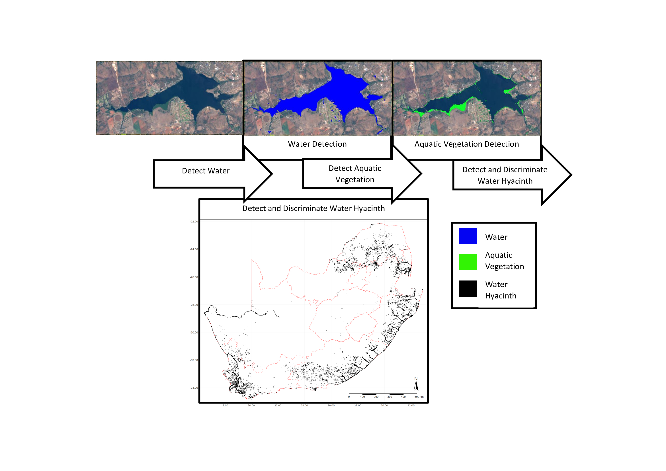
2.2. The Mapping Process

To map and discriminate between water hyacinth and other non-target species, we followed a three-stage process. During the first stage, surface water was detected using a novel MNDWI thresholding approach. In the second stage, aquatic vegetation was detected using two different methods (Otsu + Canny, and MultiResUnet semantic segmentation). In the third stage, the Otsu + Canny detected vegetation was discriminated into water hyacinth and other non-target vegetation pixels using a random forest model. Each of these stages are detailed in Figure 2. In addition, an example output from stages 1 and 2 is provided in Figure 3.

The spectral index equations of MNDWI [41], normalised difference vegetation index (NDVI,) [47], land surface water index (LSWI) and the green atmospherically resistant index (GARI, [48,49]), normalized difference aquatic vegetation index (NDAVI) used in this study are listed as Equations (1)–(5) [50].

$$MNDWI=\frac{Green-SWIR1}{Green+SWIR1}$$

(1)

$$NDVI=\frac{NIR-Red}{NIR+Red}$$

(2)

$$LSWI=\frac{NIR-SWIR1}{NIR+SWIR1}$$

(3)

$$GARI=\frac{NIR-\left(Green-\left(Blue-Red\right)\right)}{NIR-\left(Green+\left(Blue-Red\right)\right)}$$

(4)

$$NDAVI=\frac{NIR-Blue}{NIR+Blue}$$

(5)

2.2.1. Stage 1: Surface Water Detection

The automatic detection of surface water across South Africa was achieved by first deriving a 95th percentile MNDWI image composite from the Landsat-8 surface reflectance image collection (MNDWIp95), which extended from the start of the archive (2013) to the end of 2018. A 95th percentile image is computed on a per-pixel basis, i.e., all pixel values for a location are sorted in ascending order and the value corresponding to the 95th percent index position is used as the pixel value. The 95th percentile image leverages the spectral properties of clouds, water, and land surfaces that are captured by the MNDWI index. Generally, the MNDWI value of water (MNDWIw) is greater than those of clouds (MNDWIc), but the MNDWI value of clouds is greater than those of non-water areas (MNDWIo). For example, irrigated agricultural areas and shadow areas that overlap (spectrally) with MNDWI water values [51]. As a result of this relationship, i.e., MNDWIw > MNDWIc > MNDWIo, the contrast between water and cloud covered land surfaces that are frequently misclassified as water become more pronounced (Figure 4). This makes the 95th percentile MNDWI image useful for water detection. This MNDWIp95 layer was then used within an inequality (6) to detect surface water. Additional pre-processing steps included the removal of sensor anomalies and steep slopes by removing those pixels with MNDWIp95 values greater than 0.9984 or with a slope greater than 10 degrees [52]. The 0.9984 threshold was determined by manually inspecting the minimum value of scene overlap artefacts. The slope layer was derived from the Shuttle Radar Topography Mission (SRTM) elevation dataset. To produce a monthly/quarterly/annual water map, the detected water for each cloud-free image within the period of interest was superimposed.

A surface water pixel with unique coordinates x and y can be characterized by:

$$MNDWIxy\ge \left|MNDWIp95\right|-\left|MNDWIxy\right|,$$

(6)

where MNDWIxy is the MNDWI pixel value at coordinates x and y, from a single image. Since the inequality (6) utilizes a difference between two periods on the right-hand-side (RHS), this can be considered as a bi-temporal change detection component for which four scenarios need to be accounted for. These four scenarios include: (1) water remains water, i.e., LHS ≥ RHS; (2) water is gained, i.e., LHS ≥ RHS; (3) water is lost, i.e., LHS < RHS; and (4) non-water remains non-water, i.e., LHS < RHS. To satisfy all four of these scenarios, the use of absolute values on the RHS are necessary. For example, in scenario three, when water is lost at a pixel, the long term MNDWI value (MNDWIp95) will be high (closer to 1) and the MNDWI value (MNDWIxy) after the pixel has undergone a loss of water will have a low MNDWI value. Therefore, the difference between these two values (|MNDWIp95| − |MNDWIxy|) will be greater than the MNDWI value on the LHS (MNDWIxy), satisfying the inequality for scenario 3, i.e., LHS < RHS.

The accuracy of the annual detected surface water was evaluated against the annual Joint Research Centers’ (JRC) Global Surface Water product (GSW, [53]), available on Google Earth Engine, using the Intersection over Union (IoU) metric. This metric represents the ratio of the shared pixel area to the total area after merging the two datasets. For this evaluation, the maximum extent of seasonal and permanent surface water from 2013 to 2015 was compared against the water extent derived using the introduced MNDWI thresholding approach for the same period. The second evaluation involved a comparison of the 2018 surface water layer from this study and the GSW dataset, each against the 2018 South African National Land Cover field validation data points (SANLC, [54]) using a confusion matrix. To enable the comparison, all water related class points were reclassified as water (class 12–21, n = 1316) or non-water (remaining classes, n = 5254). Lastly, Sentinel-2 derived surface water masks for France were used to evaluate the method’s transferability to different platforms, and its ability to generalize to different countries [52].

2.2.2. Stage 2: Aquatic Vegetation Detection

The combination of the Otsu thresholding and Canny edge detection techniques (Otsu + Canny) have previously been used to detect water [51] by the calculation of a local, as opposed to a global, MNDWI threshold value through the Canny edge detection algorithm. This allows for a more accurate separation of water pixels from the background pixels using Otsu thresholding [55] and is achieved by determining a local threshold value that maximizes the between class variance (interclass variance).

Here, the Otsu + Canny approach was repurposed to detect aquatic vegetation. The ability to detect aquatic vegetation as opposed to water was achieved by using the water extent generated from the previous water detection stage to limit the Landsat-8 or Sentinel-2, level 1C pixels that are passed to the Otsu + Canny detector. This results in a bimodal distribution for those sites that contain aquatic vegetation and therefore, allows for the computation of a NDVI threshold value that separates water from aquatic vegetation. By limiting the detection of vegetation to the extent of open water, the confusion between aquatic vegetation and surrounding landcover, including terrestrial and riparian vegetation is reduced.

The benefit of using the Sentinel-2, Top-of-Atmosphere (TOA) product is its extended availability compared to the Bottom-of-Atmosphere (BOA) product—available outside of Europe only from December 2018. To determine if the increased atmospheric influence on the TOA derived spectral indices influenced the detection ability of aquatic vegetation, three different spectral indices with varying sensitivity to atmospheric interference were evaluated. These include, from least sensitive to most sensitive, the GARI [49], the NDVI [47], and the NDAVI, [50]. The higher sensitivity of the NDAVI index can be attributed to the blue band that is used to derive the index.

2.2.2.1. Stage 2: Semantic Segmentation—An Alternative Aquatic Vegetation Detection Method to Otsu + Canny

The detected aquatic vegetation was then used to train a semantic segmentation model. Unlike the Otsu + Canny method, a semantic segmentation model directly detects aquatic vegetation, circumventing the need to first detect water and, in this way, preventing the propagation of errors from water layers that may not always be available at a desirable spatio-temporal resolution or accuracy. The MultiResUnet architecture applied here [56], like the popular Unet model, follows the encoder-decoder model structure (architecture, [57]). During the encoder or contracting path, the image size is reduced, preserving the information that is most important for detecting aquatic vegetation. In this way, there is also a memory footprint reduction during model training. These encoder layers consist of convolution layers that assist in learning the contextual relationships, for example, between water and aquatic vegetation. During the decoder or expansive path, the feature information and spatial information are combined through a series of deconvolutions and concatenations with high-resolution features from the contracting path to allow for corresponding height and width dimensions between the input image and the output segmentation map.

The first improvement of the Unet architecture that led to the MultiResUnet architecture, included two additional convolution steps, a 3 × 3 and a 7 × 7 kernel, in addition to the usual 5 × 5 convolution, to improve the model’s capacity to cope with the detection of variable sized aquatic vegetation mats. Second, the concatenation paths, which transfer high-resolution spatial information from the encoder layers to the decoder layers, contain skip connections between added layers [56]. This assists in the alignment of deep and shallow features being assembled from the encoder and decoder [56].

2.2.2.2. Pre-Processing

We selected 462 Sentinel-2A and 2B, level 1C image scenes of Hartbeespoort dam, South Africa from the start of the Sentinel-2 archive (23rd June 2015) to the 22nd of June 2019 (~2304 pixels × 2304 pixels). Hartbeespoort dam was selected as the test area for semantic segmentation since it contains a known large infestation of water hyacinth. Moreover, it is surrounded by a heterogenous landscape, including urban infrastructure, agricultural land, and shadow areas—all of which are frequently confused with water or aquatic vegetation. Thus, the heterogenous composition of the Hartbeespoort area can more closely represent other areas of interest with a similar or less complex landcover composition. The 462 visible and near-infrared (VNIR) images were filtered to 275 images with less than 10% cloud cover. The 10 m VNIR images with corresponding Otsu + Canny aquatic vegetation masks were downloaded from GEE for each of the 275 images.

The downloaded images and corresponding masks were sliced and saved into 16-bit patches of 256 × 256 pixels to reduce the memory footprint during model training. The VNIR bands were further normalized between the range of zero to one to improve model convergence during learning. The slicing yielded 1700 patches that were then randomly split into 80% training data, 10% validation data, and 10% test data. The validation data was used for halting model fitting (early stopping), i.e., when the validation loss stopped decreasing over seven consecutive epochs, a point at which model overfitting to data noise may occur. An epoch, for training a neural network, refers to a single cycle of parameter learning from the training dataset, calculation of error (loss) against the validation dataset and subsequent update of learnt parameters for the next learning cycle. The term loss is used instead of error since a neural network outputs a probability of belonging to the target class (aquatic vegetation). The validation loss (binary cross-entropy loss) represents the mean negative log probability for the predicted probabilities. This is comparable to an error score that may be reported for discrete predicted outputs.

2.2.3. Stage 3: Species Discrimination

The GPS localities (n = 513) containing species name, waterbody name and year were linked to waterbodies within 250 m of a GPS point. This resulted in 458 waterbodies with labels, 98 of these waterbodies contained aquatic vegetation detected by Landsat-8. These final 98 waterbody extents were then used to clip the explanatory image variables (refer to

Table 1. The initial 64 explanatory variables used to fit a random forest model that discriminated between water hyacinth and other aquatic vegetation pixels.

Variable	Data Source (Year)	Spatial Resolution (m)
Seasonal median spectral bands, excluding panchromatic band 8	Landsat-8 for the respective field locality year (2013–2015)	30
Summer (12/01–02/28)
Autumn (03/01–05/31)
Winter (06/23–08/31)
Spring (09/01–11/30)
Percentiles (5,25,50,75,95) of spectral indices (NDVI, GARI, LSWI)	Landsat-8 for the respective field locality year (2013–2015)	30
Elevation	SRTM (2000)	90
Global human modification	Kennedy et al. (2019) (2016)	1000
Sum of solar radiation	Terraclimate (2013–2015)	~4670
Minimum temperature	Worldclim: bio variables (1960–1990)	1000
Temperature seasonality
Precipitation seasonality
Gross biomass water productivity	Wapor for the respective field locality year (2013–2015)	250
Actual evapotranspiration
Total biomass production

NDVI—Normalized Difference Vegetation Index [47], GARI—Green Atmospherically Resistant Index [49], LSWI—Land Surface Water Index [48], Shuttle Radar Topography Mission (SRTM).

for the list of variables). The aquatic vegetation pixels within the clipped waterbody extents were identified using the Otsu + Canny approach. Thereafter, random forest models (number of trees = 100) were calibrated and evaluated using a repeated stratified k-fold cross-validation strategy (repeats = 20, k = 5, strata = one of seven classes in Figure 1) to calculate a summed confusion matrix and the mean and standard deviation overall accuracy, F1-score and Matthews correlation coefficient (MCC) metrics. During the cross-validation, the aquatic vegetation pixels that belonged to a waterbody were constrained to either the training or testing partition, but not both partitions. This reduced the overestimation of accuracy owing to spatial autocorrelation and is referred to here as spatially constrained repeated stratified k-fold cross-validation. A random forest model consists of multiple decision trees that are grown from a random selection of explanatory variables. The final prediction is based on the most common (mode) prediction class from all decision trees.

To determine the variables that were used in the final model, a combination of variable selection techniques was employed, recursive feature elimination, permutation importance and highly correlated feature elimination. Variable selection removes redundant features, decreases computation, improves model interpretability, and may also improve model accuracy. Recursive feature elimination served to remove those variables that decreased the F1-score. Thereafter, these features were further refined by removing those variables that had a negative permutation importance score and finally, for two features that had a high correlation coefficient (>0.8), the correlated variable that had a lower permutation importance score was removed. The coarser resolution explanatory variables (human modification, minimum temperature, and precipitation seasonality) were resampled to 30 m (Landsat-8) by default within GEE using nearest neighbor resampling. The final model, fitted on the selected variables, was deployed on GEE to discriminate water hyacinth from other non-target species across South Africa.

3. Results

3.1. Evaluation of Surface Water Detection

When applying the introduced water detection approach to Landsat-8 data for South Africa and comparing the results to the maximum GSW extent for the same period of 2013 to 2015, a moderate 0.695 IoU score was obtained. A value of 1 corresponds to complete overlap between datasets. These results suggest the superior accuracy of the GSW dataset. However, when compared to the SANLC dataset, both approaches perform similarly with our method slightly outperforming the GSW dataset based on MCC (Figure 5). In addition, the confusion matrices highlight a greater commission error than omission error for both datasets.

To evaluate the introduced water detection methods’ transferability to Sentinel-2 and a different country, our method was compared to a 10 m surface water dataset for France [52]. The 10 m dataset was derived by a rule-based superpixel (RBSP) method [52]. A visual comparison of the GSW, RBSP-derived water layer and the water layer derived using the introduced method can be found here. Seasonal and smaller waterbodies were less accurately detected in comparison to the RBSP method and, to a lesser degree, the GSW layer. Note, in addition to the water detection method (Section 2.2.1), an additional post-processing step for France was carried out to reduce the commission errors with agricultural areas. This was achieved by removing pixels that had a higher NDVI value than a normalized difference water index (NDWI) value.

3.2. Evaluation of Aquatic Vegetation Detection

The Sentinel-2 TOA image collection, available on GEE, can be used to detect aquatic vegetation with superior accuracy to the BOA data despite the influence of atmospheric effects (Figure 6).

A visual comparison between the detected aquatic vegetation from the Otsu + Canny and the MultiResUnet approach showed a high correspondence with each other and their associated RGB image (Figure 7). In addition, the predicted outputs correspond to a low validation binary cross-entropy loss/error and high validation accuracy against reference aquatic vegetation generated using the Otsu + Canny algorithm (

Table 2. The training and validation mean (± SD) accuracy and binary cross entropy loss/error for the semantic segmentation (MultiResUnet) of aquatic vegetation (examples are shown in Figure 3). Note, accuracy values closer to one, and low loss values closer to zero are better and are based on Otsu + Canny reference masks. The last epochs’ scores are averaged over three iterations (lasting 94, 76, and 83 epochs each).

Training Accuracy	Validation Accuracy	Training Loss	Validation Loss
0.9814 ± 0.0030	0.9851 ± 0.0035	0.0655 ± 0.0017	0.0740 ± 0.0078

).

3.3. Evaluation of Aquatic Vegetation Discrimination

The mean and distribution values of the overall accuracy, F1-score, MCC, precision, and sensitivity metrics are based on spatially constrained repeated stratified k-fold cross-validation (Figure 8A,B). The validation data, like the calibration data, show a negative class imbalance along with the false positive and false negative occurrences for water hyacinth and non-water hyacinth pixels (Figure 8C,D). The F1-score is a weighted average of precision and recall, and thus takes into consideration both false positives and false negatives, respectively. The F1-score and MCC are much less sensitive to the class imbalances between water hyacinth (positive instances) and non-water hyacinth pixels (negative instances). However, for binary classification, especially with imbalanced data cases, the MCC metric is favored over other accuracy metrics, including the overall accuracy and F1-score metric [58] because the MCC metric is high when the majority of both the positive and negative instances have been successfully discriminated. Nevertheless, multiple metrics are reported for easier comparison with other studies.

Based on MCC, the metric that is least sensitive to class imbalance, the discrimination accuracy of water hyacinth and non-water hyacinth pixels is 0.78 (0.17) when using all 64 variables (listed in Table 1) or 0.80 (0.16) if limited to the eight most important variables (Figure 9).

Four of the eight most important variables for discriminating between water hyacinth and other aquatic vegetation are thermally related; for example, the minimum temperature in the coldest month and autumn, spring, and winter brightness temperature (top-of-atmosphere radiance). Optically active bands that feature among the top performing discriminative bands include the autumn median green band and the 95th percentile GARI (Figure 9). Moreover, by reducing the number of variables and keeping the eight most important variables, there is no loss in accuracy but rather a slight improvement in discrimination accuracy (

Table 3. Comparison of user and producer accuracy scores between studies that have mapped water hyacinth. The area of imagery (km²) that water hyacinth was mapped is provided. The area estimates (~) were not provided in the studies and were based on the bounding box of the georeferenced output classification map found within each study. The highest accuracy and greatest area shown in bold print.

Reference	Accuracy (%)		Area (km2)	Sensor (Season)
	User	Producer
[35]	67.35	67.35	~958	Landsat-7
	91.67	89.8	~958	Landsat-8
[20]	100	90	~5228	Landsat-8 (wet)
	92	90	~5228	Landsat-8 (dry)
[21]	44	50	~5228	Landsat-8
	89.3	61	~5228	Sentinel-2
[22]	76.42	94.44	~5228	Sentinel-2 (wet)
	74.67	66.04	~5228	Sentinel-2 (dry)
[19]	85	83	~18,180	Landsat-8
This study	87.48	92.98	1,219,090	Landsat-8

). Lastly, owing to the wide distribution of sites used during cross-validation, these results suggest the effectiveness for water hyacinth discrimination across wide areas (Figure 10).

The user and producer accuracy of water hyacinth is used as a comparison to previous studies since this metric is reported by all five previous studies (Table 3). This study showed superior water hyacinth discrimination results for at least one of these metrics despite the larger inference area (Table 3).

4. Discussion

We demonstrate the benefit of utilizing a hierarchical classification approach to firstly map water, then aquatic vegetation and finally water hyacinth. Additionally, we highlight the challenges associated with the MultiResUnet method for large scale mapping. The introduced hierarchical classification method relies on simple thresholding and allows for the near-instantaneous monitoring of water extent and aquatic vegetation cover over the long-term and across national extents. Subsequently, if water hyacinth infestations are closely monitored across large areas, this may assist in systematically evaluating the effectiveness of past and future management efforts. We anticipate that this GEE workflow (Figure 2) can be applied to other IAAP infested countries in a cost-effective but easy and reliable manner.

4.1. Stage 1—Surface Water Detection

The introduced MNDWI thresholding approach requires a long-term 95th percentile MNDWI image and a slope layer derived from the SRTM elevation dataset for the detection of open-water from either a Landsat-8 or Sentinel-2 cloud-free image. When the open-water images are combined for a monthly, quarterly, or annual time-period, they allow for the open-water and water areas that may have been covered by aquatic vegetation, for a portion of the temporal window of interest, to be detected.

While the GSW products are an iconic dataset ascribed to its unique global and long-term coverage (1984–2018, [53]), the introduced water detection approach provides several advantages over the GSW dataset. Both annual and monthly GSW products remain restricted to Landsat (30 m) and for the period extending from March 1984 to January 2018 [53]. While this dataset is updated, there is an update lag and a lack of publicly available update schedules. These restrictions limit the suitability of the GSW data for tracking water and aquatic vegetation on a current basis and at higher spatial resolutions when using Sentinel-2. Furthermore, the derivation of the GSW relies on an expert classification system, whcih has not yet been adapted for Sentinel-2. In addition to the expert classification system relying on the SRTM dataset for terrain shadow removal, the GSW dataset depends on additional ancillary datasets (for example, glacier data and the global human settlement layers (GHSL) for the removal of shadows cast by buildings, [53]). Therefore, there is increased computation associated with handling these datasets and an increase in the propagation of errors within the final GSW dataset. In contrast, the introduced water detection approach only requires the SRTM layer and has been shown to be applicable to both Landsat-8 data, and Sentinel-2 data. Moreover, it can be used to monitor current water dynamics of individual sites near-instantaneously and over multiple years owing to its computational efficiency (from 2013 for Landsat-8 and from 2015, within Europe, for Sentinel-2 or December 2018 outside of Europe).

Many other available water detection approaches have only been evaluated for individual satellite scenes in time and/or space (for example, [59,60,61]) and therefore show a limited generalization capacity when transferred to non-study time periods or areas. For example, supervised learning approaches are computationally expensive and sensitive to the quality and quantity of training samples, which may be difficult and costly to obtain. Our MNDWI thresholding approach overcomes these limitations and can generalize across time for the same area or to different areas while remaining simple to execute. This can be attributed to the nature of the thresholding method, i.e., it does not require labelled data or model fitting.

The moderate IoU score (0.695) between the 2013–2015 GSW layer (reference) and the water layer derived using this method may partly be attributed to the misalignment issue of the GSW data—due west across South Africa. Furthermore, omission and commission errors in both water products may have also contributed to the IoU score. For the GSW product, an omission error of less than 5% was reported, however, this was based on 40,000 reference points distributed globally [53]. Since points are not a comprehensive evaluation of all pixels, it is likely that there are omission and commission errors that are not accounted for by the points. This is supported by the GSW omission errors reported in recent studies that compared satellite detected water from higher resolution data [52,62]. Wu et al. 2019 [62] have shown considerable omission errors in the GSW product when compared to 1 m detected surface water. Furthermore, Yang et al. (2020) [52], reported a 25% omission error in the GSW product when compared to Sentinel-2 derived water (10 m) for France. Lastly, based on a comparison with the 2018 SANLC dataset (Figure 5), there is a much higher omission error compared to the commission error for both the GSW dataset and the introduced dataset. These studies and results highlight the role of spatial resolution and the difficulty in mapping smaller, seasonal surface water features that account for most misclassification errors between the GSW water product and the water layer derived using the introduced approach. Despite the moderate IoU score, and the difficulty in identifying smaller seasonal waterbodies, the introduced water detection method is valuable for current and near-instantaneous monitoring of large, less seasonal surface waterbodies that are of higher priority for IAAP species monitoring, especially when the GSW data is unavailable.

To compensate for the seasonal dynamics of water and improve aquatic vegetation detection, a more frequent water detection product is required. Whilst the GSW product provides a monthly dataset, it is highly sensitive to the presence of aquatic vegetation, ascribed to the relatively low 16-day temporal resolution of Landsat [53]. As a result, it is less suitable for detecting aquatic vegetation based on the introduced hierarchical classification method. For this reason, Sentinel-2, with a higher temporal resolution (up to 2–3 days), is preferable for aquatic vegetation detection.

4.2. Stage 2—Aquatic Vegetation Detection

Aside from the occasional artefacts present when using the BOA data, it also overestimates the detected aquatic vegetation compared to the TOA product. Moreover, the aquatic vegetation derived from the different indices using either the L1C or L2A data product show high agreement within a product (L1C or L2A) and across the different indices. The results suggest that the TOA data with atmospheric influences have an improved water and aquatic vegetation separability, and therefore outperform the BOA data for aquatic vegetation detection (Figure 6). A basic analysis of the histograms for TOA and BOA-derived NDVI images that contained water and aquatic vegetation revealed a consistent pattern whereby the BOA NDVI had a greater range than the TOA-derived NDVI. This has been attributed to the adjacency effect and contrast degradation [63,64]. Contrast degradation as part of the adjacency effect refers to the introduction of systematic noise when there is a strong water reflectance contrast [65], in this case, with aquatic vegetation. Overall, this leads to a larger number of water pixels being falsely detected as aquatic vegetation in the BOA data because of the increased spectral overlap with aquatic vegetation pixels. As a result, the TOA data outperforms the BOA data for the detection of aquatic vegetation using the Otsu + Canny method.

Semantic segmentation is proposed as an alternative approach to detect aquatic vegetation. A semantic segmentation model trained to detect aquatic vegetation benefits from the ability to directly detect aquatic vegetation, without the need to first detect water and then detect aquatic vegetation like the Otsu + Canny method. This is valuable since EO-based water detection is confronted by numerous complexities and inaccuracies that are propagated from ancillary layers, placing an upper bound on the accuracy of aquatic vegetation detection when using Otsu + Canny in a hierarchical classification framework. When an inaccurate water boundary is provided for aquatic vegetation detection, the Otsu + Canny method results in less accurate aquatic vegetation maps in comparison to those derived using the MultiResUnet model.

The achievements of CNN-based semantic segmentation architectures can be ascribed to these models automating the extraction and organization of discriminative features at multiple levels of representation (from edges to entire objects) exclusively from input data, without the need for additional user input [66]. This ability of CNNs to learn high level features takes advantage of both the spatial context of land-cover and the spectral features in an invariant manner—unlike pixel-based and object-based approaches [67]. Furthermore, traditional approaches require additional features to be manually engineered and can thus be time consuming to design and validate, especially for large areas [68] and may still result in sub-optimal discrimination features. For example, there is no consensus on the most suitable spectral water index to detect water—this points to manual features that may perform sub-optimally depending on the waters’ optical properties, study area location, and the varying quality and properties of satellite imagery [69]. Secondly, the deep nature (numerous layers) of CNN models, which allow for a variety of simple to highly complex, hierarchical, and non-linear features to be learnt from large amounts of data, allow for improved model prediction power [70]. Owing to the increase in model prediction power and the associated increases in model complexity and computational requirements, CNN models generally require costly hardware, which may not always be available. Subsequently, the presented hierarchical classification scheme used to detect aquatic vegetation offers a cost-effective, scalable, and accurate but simple alternative to detect aquatic vegetation for large volumes of EO data.

In terms of the accuracy of either approach, no independent and publicly available datasets exist with which to compare the detected area of aquatic vegetation. However, based on the comparative visual inspection (Figure 7) and calculated accuracy of the MultiResUnet detected aquatic vegetation against the reference masks generated by the Otsu + Canny algorithm (Table 2), both approaches show very high correspondence with each other and their associated RGB image. Lastly, the generated aquatic vegetation masks may be combined with existing water products to alleviate omission errors arising from aquatic vegetation cover; for example, the GSW monthly water product [53].

4.3. Stage 3—Species Discrimination

The use of the percentile spectral index bands (95th percentile GARI) together with the median seasonal bands (spring green band—50th percentile) assisted in capturing the phenological characteristics of water hyacinth and have been used to accommodate the intra-species variance in phenological patterns across large extents. Moreover, median images (50th percentile) have been shown to be valuable in reducing data volume while providing important discrimination information [13]. Simultaneously, four of the eight final variables used in the final model included thermal related bands and highlight the importance of including environmental variables that take into consideration the target plant species’ thermal physiology when discriminating between IAAPs using EO data. The growth of water hyacinth has been shown to be strongly linked to temperature, where the plant starts to brown and die back at temperatures below 10 °C [16]. Therefore, the importance of the minimum temperature (in the coldest month) variable aligns with known water hyacinth thermal physiology and further suggests that the model has learnt valid relationships. Note, the four thermal-related variables had a correlation below 0.8 between each other most likely because they represent different temporal windows. The minimum temperature variable relates to climate while the remaining three temperature variables relate to seasonal weather. Moreover, the minimum temperature variable that had a correlation coefficient greater than 0.8 with elevation, represents a broader temporal (> 30 years) and spatial scale (1 km resampled to 30 m) as compared to the brightness temperature bands (seasonal median bands at 100 m resampled and provided at a 30 m spatial resolution). Note, the correlation coefficients are based on the entire training and validation dataset partitions.

It is difficult to reliably compare the water hyacinth discrimination results of this study against previous studies owing to the different goals and evaluation approaches. For example, previous studies aimed to generalize within fewer study sites distributed across smaller study areas [20,21,22,35], whilst this study aimed to generalize across different study sites distributed across a large study area. In addition, most previous studies [20,21,22,35] aimed to discriminate surrounding terrestrial land cover and water from water hyacinth and Cyperus papyrus [19], whereas this study focused on discriminating water hyacinth from other aquatic vegetation. As a result of the easier classification goal, our method was able to map water hyacinth at superior accuracies for at least one accuracy metric (user accuracy or producer accuracy), despite the study area being 67 times greater than previous attempts (Table 3).

4.4. Management Tools

The monitoring tools generated in this study are made available within GEE (here) and will allow users to track the extent of water and aquatic vegetation within a waterbody from 2013 to present using Landsat-8 (30 m) or when using Sentinel-2, from 2015, within Europe or from December 2018 outside Europe at 10 m (aquatic vegetation) and 20 m (water) (script name: Aquatic vegetation and water monitor). Users will also be able to generate a larger national extent overview of aquatic vegetation cover using Landsat-8 (script name: National Extent Vegetation Detection L8) or Sentinel-2 (script name: National Extent Vegetation Detection S2). Lastly, the 2013 species-level distribution of water hyacinth across South Africa has been made available as a raster layer within GEE (script name: 2013 water hyacinth distribution) together with the field locality data used for model calibration and validation. We anticipate that these data products will assist in management prioritization, control measure implementation, and subsequently the tracking of past, present, and future (in)effectiveness of these control efforts.

4.5. User Guidelines, Caveats, and Limitations

Since the proposed water detection approach relies on a long-term MNDWI percentile image, the introduced approach remains most suitable to optical imaging systems with archived imagery. In addition, the duration between successive water maps may vary from two to three days under optimum conditions, i.e., cloud-free conditions and vegetation-free water sites. Or may decline to monthly, quarterly, or annually in the presence of clouds or stationary aquatic vegetation mats. Both these factors may hinder the detection of the actual water surface extent and therefore, the ability to accurately monitor water and aquatic vegetation dynamics. These are limitations experienced by other water detection approaches that utilize optical data for surface water detection [53,71]. Generally, the more frequently water can be mapped, the better the accommodation of changes in water extent, and the greater the accuracy of the aquatic vegetation detection. For example, if the detected waterbody extent is less than the actual extent, the area of aquatic vegetation is likely to be underestimated, and vice versa. If the detected waterbody is greater than the actual extent, then riparian vegetation or previously inundated land may falsely be identified as aquatic vegetation.

Since a pixel-level classification was used to detect and discriminate aquatic vegetation from explanatory variables with a 30 m spatial resolution, an isolated 30 m pixel may be identified as water hyacinth and represents the area of the minimum detectable water hyacinth canopy for Landsat-8 (i.e., 30 m × 30 m). Given this, smaller (<30 m × 30 m) isolated mats have a lower probability of being detected. Smaller undetected mats are important for an improved chance of successful management. As a result, there may be delays in early detection of water hyacinth mats until the mats grow to an EO-detectable size. This limitation should be considered when using the introduced workflow to monitor smaller water hyacinth infestations. At the same time, it may be very costly to monitor water hyacinth at higher spatial resolutions and at a similar frequency of Landsat-8 or Sentinel-2. Currently, it is feasible to monitor large infestations with the available medium resolution EO data from Landsat-8 and Sentinel-2.

Species reference localities from the field are valuable for reliably assessing the accuracy of EO derived water, aquatic vegetation, and IAAP species distribution maps. However, existing field locality data is often less suitable for high spatial resolution distribution maps compared to other EO applications, e.g., habitat suitability modelling [72]. Field data may be clustered in some areas and sparse or not available in other areas (Figure 1). This is evident when comparing the EO derived water hyacinth distribution (Figure 10) against the field locality data (Figure 1). Other compatibility challenges that were encountered with the field locality data in this study (similarly encountered and outlined by Vorster et al., 2018 [72]) included geo-registration errors (i.e., points were located outside the boundary of waterbodies) and/or opportunistic data capture errors (i.e., GPS points may have been taken outside waterbodies, on nearby roads). The inaccuracy effects of these points were minimized by linking them to waterbodies that were up to a maximum distance of 250 m away. Additionally, those field locality points that were recorded for moving IAAP mats could reduce the spatial correspondence between imagery and field data owing to the time lag between image capture and field data capture. By linking these field localities to entire waterbodies, this was avoided. The lag period between satellite image capture and field data capture could potentially be up to a year for this study. This could have resulted in noise within the training data that was used to fit the random forest model and could potentially explain some of the misclassification error reported.

5. Recommendations and Conclusions

We have introduced a hierarchical classification approach that enables the near-instantaneous monitoring of water and aquatic vegetation on a frequent basis. This approach has also allowed for the first EO-derived distribution of water hyacinth on a national extent. We have also discussed the opportunities introduced by the proposed workflow to circumvent labelling costs associated with CNN-based aquatic vegetation detection. This would consequently remove the need for surface water masks that may not always be available at the required spatio-temporal resolution or accuracy. Whilst we have shown encouraging results for the MultiResUnet-based detection of aquatic vegetation within a single heterogenous study area, the computational infrastructure required for the operational CNN-based mapping of aquatic vegetation across large extents remains a challenge. Therefore, this study suggests that the hierarchical classification approach is advantageous over a CNN based approach for the final goal of mapping water hyacinth since it greatly reduces commission errors in comparison to previous approaches. In addition, the need for remote sensing practitioners to establish high quality reference datasets that will enable a more consistent and reliable comparison of mapping methods and their associated results in a systematic manner across studies is highlighted. Greater effort needs to be placed on obtaining reference data for other IAAP species since our results, similar to previous studies [73,74], highlight the spectral separability of water hyacinth from the other IAAP species that were represented in the non-target species class. Lastly, the value of using species appropriate variables, such as minimum temperature, was shown to be highly valuable. Overall, this study suggests that EO data is highly suitable for an IAAP monitoring programme. The recommendations made in this study are likely to be applicable to EO-based monitoring of invasive terrestrial alien plants.

References

1. Strayer, D.L.; Dudgeon, D. Freshwater Biodiversity Conservation: Recent Progress and Future Challenges. J. N. Am. Benthol. Soc. 2010, 29, 344–358. [Google Scholar] [CrossRef] [Green Version]
2. Ricciardi, A.; MacIsaac, H.J. Impacts of Biological Invasions on Freshwater Ecosystems. In Fifty Years of Invasion Ecology: The Legacy of Charles Elton; Wiley: Hoboken, NJ, USA, 2011; pp. 211–224. [Google Scholar]
3. Rejmánek, M.; Pitcairn, M.J. When is eradication of exotic pest plants a realistic goal. In Turning the Tide: The Eradication of Invasive Species: Proceedings of the International Conference on Eradication of Island Invasives; Veitch, C.R., Clout, M.N., Eds.; IUCN: Cambridge, UK, 2002; pp. 249–253. [Google Scholar]
4. Vila, M.; Ibáñez, I. Plant Invasions in the Landscape. Landsc. Ecol. 2011, 26, 461–472. [Google Scholar] [CrossRef]
5. Nielsen, C.; Ravn, H.P.; Nentwig, W.; Wade, M. (Eds.) The Giant Hogweed Best Practice Manual. Guidelines for the Management and Control of an Invasive Weed in Europe; Forest and Landscape Denmark: Hørsholm, Denmark, 2005; pp. 1–44. ISBN 87-7903-209-5. [Google Scholar]
6. Pyšek, P.; Hulme, P.E. Spatio-Temporal Dynamics of Plant Invasions: Linking Pattern to Process. Ecoscience 2005, 12, 302–315. [Google Scholar] [CrossRef]
7. Wittenberg, R.; Cock, M.J.W. Best Practices for the Prevention and Management of Invasive Alien Species. In Invasive Alien Species: A New Synthesis; Island Press: Washington, DC, USA, 2005; pp. 209–232. [Google Scholar]
8. Richardson, D.M.; Foxcroft, L.C.; Latombe, G.; Le Maitre, D.C.; Rouget, M.; Wilson, J.R. The Biogeography of South African Terrestrial Plant Invasions. In Biological Invasions in South Africa; Springer: Berlin/Heidelberg, Germany, 2020; pp. 67–96. [Google Scholar]
9. Wallace, R.D.; Bargeron, C.T.; Ziska, L.; Dukes, J. Identifying Invasive Species in Real Time: Early Detection and Distribution Mapping System (EDDMapS) and Other Mapping Tools. Invasive Species Glob. Clim. Chang. 2014, 4, 219. [Google Scholar]
10. Li, J.; Roy, D.P. A Global Analysis of Sentinel-2A, Sentinel-2B and Landsat-8 Data Revisit Intervals and Implications for Terrestrial Monitoring. Remote Sens. 2017, 9, 902. [Google Scholar]
11. Cohen, W.B.; Goward, S.N. Landsat’s Role in Ecological Applications of Remote Sensing. Bioscience 2004, 54, 535–545. [Google Scholar] [CrossRef]
12. Gorelick, N.; Hancher, M.; Dixon, M.; Ilyushchenko, S.; Thau, D.; Moore, R. Google Earth Engine: Planetary-Scale Geospatial Analysis for Everyone. Remote Sens. Environ. 2017, 202, 18–27. [Google Scholar] [CrossRef]
13. Phan, T.N.; Kuch, V.; Lehnert, L.W. Land Cover Classification Using Google Earth Engine and Random Forest Classifier—The Role of Image Composition. Remote Sens. 2020, 12, 2411. [Google Scholar] [CrossRef]
14. Persello, C.; Stein, A. Deep Fully Convolutional Networks for the Detection of Informal Settlements in VHR Images. IEEE Geosci. Remote Sens. Lett. 2017, 14, 2325–2329. [Google Scholar] [CrossRef]
15. Wolter, P.T.; Mladenoff, D.J.; Host, G.E.; Crow, T.R. Using Multi-Temporal Landsat Imagery. Photogramm. Eng. Remote Sens. 1995, 61, 1129–1143. [Google Scholar]
16. Byrne, M.; Hill, M.; Robertson, M.; King, A.; Katembo, N.; Wilson, J.; Brudvig, R.; Fisher, J.; Jadhav, A. Integrated Management of Water Hyacinth in South Africa; WRC Report No. TT 454/10; Water Research Commission: Pretoria, South Africa, 2010; 285p. [Google Scholar]
17. Estes, L.D.; Okin, G.S.; Mwangi, A.G.; Shugart, H.H. Habitat Selection by a Rare Forest Antelope: A Multi-Scale Approach Combining Field Data and Imagery from Three Sensors. Remote Sens. Environ. 2008, 112, 2033–2050. [Google Scholar] [CrossRef]
18. Bradley, B.A.; Mustard, J.F. Identifying Land Cover Variability Distinct from Land Cover Change: Cheatgrass in the Great Basin. Remote Sens. Environ. 2005, 94, 204–213. [Google Scholar] [CrossRef]
19. Mukarugwiro, J.A.; Newete, S.W.; Adam, E.; Nsanganwimana, F.; Abutaleb, K.A.; Byrne, M.J. Mapping Distribution of Water Hyacinth (Eichhornia Crassipes) in Rwanda Using Multispectral Remote Sensing Imagery. Afr. J. Aquat. Sci. 2019, 44, 339–348. [Google Scholar] [CrossRef]
20. Dube, T.; Mutanga, O.; Sibanda, M.; Bangamwabo, V.; Shoko, C. Testing the Detection and Discrimination Potential of the New Landsat 8 Satellite Data on the Challenging Water Hyacinth (Eichhornia Crassipes) in Freshwater Ecosystems. Appl. Geogr. 2017, 84, 11–22. [Google Scholar] [CrossRef]
21. Thamaga, K.H.; Dube, T. Testing Two Methods for Mapping Water Hyacinth (Eichhornia Crassipes) in the Greater Letaba River System, South Africa: Discrimination and Mapping Potential of the Polar-Orbiting Sentinel-2 MSI and Landsat 8 OLI Sensors. Int. J. Remote Sens. 2018, 39, 8041–8059. [Google Scholar] [CrossRef]
22. Thamaga, K.H.; Dube, T. Understanding Seasonal Dynamics of Invasive Water Hyacinth (Eichhornia Crassipes) in the Greater Letaba River System Using Sentinel-2 Satellite Data. GIScience Remote Sens. 2019, 56, 1355–1377. [Google Scholar] [CrossRef]
23. Ingole, N.A.; Nain, A.S.; Kumar, P.; Chalal, R. Monitoring and Mapping Invasive Aquatic Weed Salvinia Molesta Using Multispectral Remote Sensing Technique in Tumaria Wetland of Uttarakhand, India. J. Indian Soc. Remote Sens. 2018, 46, 863–871. [Google Scholar] [CrossRef]
24. Hill, M.P.; Coetzee, J.A.; Martin, G.D.; Smith, R.; Strange, E.F. Invasive Alien Aquatic Plants in South African Freshwater Ecosystems. In Biological Invasions in South Africa; Springer: Berlin/Heidelberg, Germany, 2020; pp. 97–114. [Google Scholar]
25. Coetzee, J.A.; Hill, M.P.; Byrne, M.J.; Bownes, A. A Review of the Biological Control Programmes on Eichhornia Crassipes (C. Mart.) Solms (Pontederiaceae), Salvinia Molesta DS Mitch.(Salviniaceae), Pistia Stratiotes L.(Araceae), Myriophyllum Aquaticum (Vell.) Verdc.(Haloragaceae) and Azolla Filiculoides L. Afr. Entomol. 2011, 19, 451–468. [Google Scholar] [CrossRef]
26. Jones, R.W.; Cilliers, C.J. Integrated Control of Water Hyacinth on the Nseleni/Mposa Rivers and Lake Nsezi in KwaZulu-Natal, South Africa. In Biological and Integrated Control of Water Hyacinth, Eichhornia crassipes. ACIAR Proceedings; Julian, M.H., Hill, M.P., Center, T.D., Ding, J., Eds.; Australian Centre for International Agricultural Research: Canberra, Australia, 2001; Volume 102, pp. 123–129. [Google Scholar]
27. Manfreda, S.; McCabe, M.F.; Miller, P.E.; Lucas, R.; Pajuelo Madrigal, V.; Mallinis, G.; Ben Dor, E.; Helman, D.; Estes, L.; Ciraolo, G. On the Use of Unmanned Aerial Systems for Environmental Monitoring. Remote Sens. 2018, 10, 641. [Google Scholar] [CrossRef] [Green Version]
28. Dvořák, P.; Müllerová, J.; Bartaloš, T.; Brůna, J. Unmanned aerial vehicles for alien plant species detection and monitoring. Int. Arch. Photogramm. Remote Sens. Spat. Inf. Sci. 2016, 41, 903–908. [Google Scholar] [CrossRef] [Green Version]
29. Müllerová, J.; Pergl, J.; Pyšek, P. Remote Sensing as a Tool for Monitoring Plant Invasions: Testing the Effects of Data Resolution and Image Classification Approach on the Detection of a Model Plant Species Heracleum Mantegazzianum (Giant Hogweed). Int. J. Appl. Earth Obs. Geoinf. 2013, 25, 55–65. [Google Scholar] [CrossRef]
30. Joshi, C.; de Leeuw, J.; van Duren, I.C. Remote Sensing and GIS Applications for Mapping and Spatial Modeling of Invasive Species. In Proceedings of the XXth ISPRS Congress, Istanbul, Turkey, 12–23 July 2004; pp. 669–677. [Google Scholar]
31. Thamaga, K.H.; Dube, T. Remote Sensing of Invasive Water Hyacinth (Eichhornia Crassipes): A Review on Applications and Challenges. Remote Sens. Appl. Soc. Environ. 2018, 10, 36–46. [Google Scholar] [CrossRef]
32. Vaz, A.S.; Alcaraz-Segura, D.; Campos, J.C.; Vicente, J.R.; Honrado, J.P. Managing Plant Invasions through the Lens of Remote Sensing: A Review of Progress and the Way Forward. Sci. Total Environ. 2018, 642, 1328–1339. [Google Scholar] [CrossRef]
33. Rahel, F.J. Homogenization of Freshwater Faunas. Annu. Rev. Ecol. Syst. 2002, 33, 291–315. [Google Scholar] [CrossRef] [Green Version]
34. Sala, O.E.; Chapin, F.S.; Armesto, J.J.; Berlow, E.; Bloomfield, J.; Dirzo, R.; Huber-Sanwald, E.; Huenneke, L.F.; Jackson, R.B.; Kinzig, A. Global Biodiversity Scenarios for the Year 2100. Science 2000, 287, 1770–1774. [Google Scholar] [CrossRef]
35. Dube, T.; Mutanga, O.; Sibanda, M.; Bangamwabo, V.; Shoko, C. Evaluating the Performance of the Newly-Launched Landsat 8 Sensor in Detecting and Mapping the Spatial Configuration of Water Hyacinth (Eichhornia Crassipes) in Inland Lakes, Zimbabwe. Phys. Chem. Earth Parts A/b/c 2017, 100, 101–111. [Google Scholar] [CrossRef]
36. Cheruiyot, E.; Menenti, M.; Gerte, B.; Koenders, R. Accuracy and Precision of Algorithms to Determine the Extent of Aquatic Plants: Empirical Sealing of Spectral Indices vs. Spectral Unmixing. ESASP 2013, 722, 85. [Google Scholar]
37. Truong, T.T.A.; Hardy, G.E.S.J.; Andrew, M.E. Contemporary Remotely Sensed Data Products Refine Invasive Plants Risk Mapping in Data Poor Regions. Front. Plant Sci. 2017, 8, 770. [Google Scholar] [CrossRef] [Green Version]
38. Agutu, P.O.; Gachari, M.K.; Mundia, C.N. An Assessment of the Role of Water Hyacinth in the Water Level Changes of Lake Naivasha Using GIS and Remote Sensing. Am. J. Remote Sens. 2018, 6, 74–88. [Google Scholar] [CrossRef]
39. Zhang, Y.; Jeppesen, E.; Liu, X.; Qin, B.; Shi, K.; Zhou, Y.; Thomaz, S.M.; Deng, J. Global Loss of Aquatic Vegetation in Lakes. Earth Sci. Rev. 2017, 173, 259–265. [Google Scholar] [CrossRef]
40. Hill, M.P.; Coetzee, J. The Biological Control of Aquatic Weeds in South Africa: Current Status and Future Challenges. Bothalia Afr. Biodivers. Conserv. 2017, 47, 1–12. [Google Scholar] [CrossRef]
41. Xu, H. Modification of Normalised Difference Water Index (NDWI) to Enhance Open Water Features in Remotely Sensed Imagery. Int. J. Remote Sens. 2006, 27, 3025–3033. [Google Scholar] [CrossRef]
42. Henderson, L. Alien Weeds And Invasive Plants: A Complete Guide to Declared Weeds and Invaders in South Africa; Plant Protection Research Institute Handbook No. 12; Agricultural Research Council: Pretoria, South Africa, 2001. [Google Scholar]
43. Coetzee, J.; Mostert, E. (Rhodes University, Centre for Biological Control). GPS Localities for Invasive Aquatic Alien Plants (IAAPs) as a Google Earth Engine Feature Collection. Available online: https://code.earthengine.google.com/?asset=users/geethensingh/IAAP_localities (accessed on 13 June 2019).
44. Van Wilgen, B.W.; Richardson, D.M.; Le Maitre, D.C.; Marais, C.; Magadlela, D. The Economic Consequences of Alien Plant Invasions: Examples of Impacts and Approaches to Sustainable Management in South Africa. Environ. Dev. Sustain. 2001, 3, 145–168. [Google Scholar] [CrossRef]
45. Henderson, L.; Cilliers, C.J. Invasive Aquatic Plants: A Guide to the Identification of the Most Important and Potentially Dangerous Invasive Aquatic and Wetland Plants in South Africa; Also Featuring the Biological Control of the Five Worst Aquatic Weeds; ARC-Plant Protection Research Inst.: Pretoria, South Africa, 2002. [Google Scholar]
46. Richardson, D.M.; Van Wilgen, B.W. Invasive Alien Plants in South Africa: How Well Do We Understand the Ecological Impacts?: Working for Water. S. Afr. J. Sci. 2004, 100, 45–52. [Google Scholar]
47. Tucker, C.J. Red and Photographic Infrared Linear Combinations for Monitoring Vegetation. Remote Sens. Environ. 1979, 8, 127–150. [Google Scholar] [CrossRef] [Green Version]
48. Xiao, X.; Boles, S.; Frolking, S.; Salas, W.; Moore Iii, B.; Li, C.; He, L.; Zhao, R. Observation of Flooding and Rice Transplanting of Paddy Rice Fields at the Site to Landscape Scales in China Using VEGETATION Sensor Data. Int. J. Remote Sens. 2002, 23, 3009–3022. [Google Scholar] [CrossRef]
49. Gitelson, A.A.; Kaufman, Y.J.; Stark, R.; Rundquist, D. Novel Algorithms for Remote Estimation of Vegetation Fraction. Remote Sens. Environ. 2002, 80, 76–87. [Google Scholar] [CrossRef] [Green Version]
50. Villa, P.; Laini, A.; Bresciani, M.; Bolpagni, R. A Remote Sensing Approach to Monitor the Conservation Status of Lacustrine Phragmites Australis Beds. Wetl. Ecol. Manag. 2013, 21, 399–416. [Google Scholar] [CrossRef]
51. Donchyts, G.; Baart, F.; Winsemius, H.; Gorelick, N.; Kwadijk, J.; Van De Giesen, N. Earth’s Surface Water Change over the Past 30 Years. Nat. Clim. Chang. 2016, 6, 810–813. [Google Scholar] [CrossRef]
52. Yang, X.; Qin, Q.; Yésou, H.; Ledauphin, T.; Koehl, M.; Grussenmeyer, P.; Zhu, Z. Monthly Estimation of the Surface Water Extent in France at a 10-m Resolution Using Sentinel-2 Data. Remote Sens. Environ. 2020, 244, 111803. [Google Scholar] [CrossRef]
53. Pekel, J.-F.; Cottam, A.; Gorelick, N.; Belward, A.S. High-Resolution Mapping of Global Surface Water and Its Long-Term Changes. Nature 2016, 540, 418–422. [Google Scholar] [CrossRef]
54. GEOTERRAIMAGE. SANLC. Accuracy Assessment Points. 2018. Available online: https://egis.environment.gov.za/data_egis/data_download/current (accessed on 28 March 2020).
55. Otsu, N. A Threshold Selection Method from Gray-Level Histograms. IEEE Trans. Syst. Man. Cybern. 1979, 9, 62–66. [Google Scholar] [CrossRef] [Green Version]
56. Ibtehaz, N.; Rahman, M.S. MultiResUNet: Rethinking the U-Net Architecture for Multimodal Biomedical Image Segmentation. Neural Netw. 2020, 121, 74–87. [Google Scholar] [CrossRef] [PubMed]
57. Litjens, G.; Kooi, T.; Bejnordi, B.E.; Setio, A.A.A.; Ciompi, F.; Ghafoorian, M.; Van Der Laak, J.A.; Van Ginneken, B.; Sánchez, C.I. A Survey on Deep Learning in Medical Image Analysis. Med. Image Anal. 2017, 42, 60–88. [Google Scholar] [CrossRef] [PubMed] [Green Version]
58. Chicco, D.; Jurman, G. The Advantages of the Matthews Correlation Coefficient (MCC) over F1 Score and Accuracy in Binary Classification Evaluation. BMC Genom. 2020, 21, 6. [Google Scholar] [CrossRef] [Green Version]
59. Qiao, C.; Luo, J.; Sheng, Y.; Shen, Z.; Zhu, Z.; Ming, D. An Adaptive Water Extraction Method from Remote Sensing Image Based on NDWI. J. Indian Soc. Remote Sens. 2012, 40, 421–433. [Google Scholar] [CrossRef]
60. Acharya, T.D.; Lee, D.H.; Yang, I.T.; Lee, J.K. Identification of Water Bodies in a Landsat 8 OLI Image Using a J48 Decision Tree. Sensors 2016, 16, 1075. [Google Scholar] [CrossRef] [Green Version]
61. Wang, Z.; Liu, J.; Li, J.; Zhang, D.D. Multi-Spectral Water Index (MuWI): A Native 10-m Multi-Spectral Water Index for Accurate Water Mapping on Sentinel-2. Remote Sens. 2018, 10, 1643. [Google Scholar] [CrossRef] [Green Version]
62. Wu, Q.; Lane, C.R.; Li, X.; Zhao, K.; Zhou, Y.; Clinton, N.; DeVries, B.; Golden, H.E.; Lang, M.W. Integrating LiDAR Data and Multi-Temporal Aerial Imagery to Map Wetland Inundation Dynamics Using Google Earth Engine. Remote Sens. Environ. 2019, 228, 1–13. [Google Scholar] [CrossRef] [Green Version]
63. Zhang, H.K.; Roy, D.P.; Yan, L.; Li, Z.; Huang, H.; Vermote, E.; Skakun, S.; Roger, J.-C. Characterization of Sentinel-2A and Landsat-8 Top of Atmosphere, Surface, and Nadir BRDF Adjusted Reflectance and NDVI Differences. Remote Sens. Environ. 2018, 215, 482–494. [Google Scholar] [CrossRef]
64. Roy, D.P.; Kovalskyy, V.; Zhang, H.K.; Vermote, E.F.; Yan, L.; Kumar, S.S.; Egorov, A. Characterization of Landsat-7 to Landsat-8 Reflective Wavelength and Normalized Difference Vegetation Index Continuity. Remote Sens. Environ. 2016, 185, 57–70. [Google Scholar] [CrossRef] [PubMed] [Green Version]
65. Frouin, R.J.; Franz, B.A.; Ibrahim, A.; Knobelspiesse, K.; Ahmad, Z.; Cairns, B.; Chowdhary, J.; Dierssen, H.M.; Tan, J.; Dubovik, O. Atmospheric Correction of Satellite Ocean-Color Imagery during the PACE Era. Front. Earth Sci. 2019, 7, 145. [Google Scholar] [CrossRef] [Green Version]
66. Zhu, X.X.; Tuia, D.; Mou, L.; Xia, G.-S.; Zhang, L.; Xu, F.; Fraundorfer, F. Deep Learning in Remote Sensing: A Comprehensive Review and List of Resources. IEEE Geosci. Remote Sens. Mag. 2017, 5, 8–36. [Google Scholar] [CrossRef] [Green Version]
67. Long, J.; Shelhamer, E.; Darrell, T. Fully Convolutional Networks for Semantic Segmentation. In Proceedings of the IEEE Conference on Computer Vision and Pattern Recognition, Boston, MA, USA, 7–12 June 2015; pp. 3431–3440. [Google Scholar]
68. Wurm, M.; Stark, T.; Zhu, X.X.; Weigand, M.; Taubenböck, H. Semantic Segmentation of Slums in Satellite Images Using Transfer Learning on Fully Convolutional Neural Networks. ISPRS J. Photogramm. Remote Sens. 2019, 150, 59–69. [Google Scholar] [CrossRef]
69. Zhou, Y.; Dong, J.; Xiao, X.; Xiao, T.; Yang, Z.; Zhao, G.; Zou, Z.; Qin, Y. Open Surface Water Mapping Algorithms: A Comparison of Water-Related Spectral Indices and Sensors. Water 2017, 9, 256. [Google Scholar] [CrossRef]
70. Ball, J.E.; Anderson, D.T.; Chan, C.S. Comprehensive Survey of Deep Learning in Remote Sensing: Theories, Tools, and Challenges for the Community. J. Appl. Remote Sens. 2017, 11, 42609. [Google Scholar] [CrossRef] [Green Version]
71. Mueller, N.; Lewis, A.; Roberts, D.; Ring, S.; Melrose, R.; Sixsmith, J.; Lymburner, L.; McIntyre, A.; Tan, P.; Curnow, S. Water Observations from Space: Mapping Surface Water from 25 Years of Landsat Imagery across Australia. Remote Sens. Environ. 2016, 174, 341–352. [Google Scholar] [CrossRef] [Green Version]
72. Vorster, A.G.; Woodward, B.D.; West, A.M.; Young, N.E.; Sturtevant, R.G.; Mayer, T.J.; Girma, R.K.; Evangelista, P.H. Tamarisk and Russian Olive Occurrence and Absence Dataset Collected in Select Tributaries of the Colorado River for 2017. Data 2018, 3, 42. [Google Scholar] [CrossRef] [Green Version]
73. Everitt, J.H.; Yang, C.; Summy, K.R.; Owens, C.S.; Glomski, L.M.; Smart, R.M. Using in Situ Hyperspectral Reflectance Data to Distinguish Nine Aquatic Plant Species. Geocarto Int. 2011, 26, 459–473. [Google Scholar] [CrossRef]
74. Everitt, J.H.; Summy, K.R.; Glomski, L.M.; Owens, C.S.; Yang, C. Spectral Reflectance and Digital Image Relations among Five Aquatic Weeds. Subtrop. Plant Sci. 2009, 61, 15–23. [Google Scholar]
Figure 1. The field localities of five invasive aquatic alien plant (IAAP) species for 2013–2015 across 98 sites within South Africa including sites with detected aquatic vegetation but none of the five IAAPs (Unpublished data, [43]). The period, 2013–2015 corresponds to a temporal window of concurrent availability of both the Landsat-8 satellite data and the field IAAP locality data. Note, the strong imbalance between the seven classes in favor of water hyacinth and against the other IAAP species. As a result, the water hyacinth localities were used as the target (positive) class whilst the remaining categories were combined to form the non-target (negative) class.
Remotesensing 12 04021 g001
Figure 2. The general workflow used in this study to map and discriminate between invasive aquatic alien plant species across South Africa with input and terminal output data (green rectangles), intermediate outputs (white rectangles) and processes (parallelograms). The dashed arrow indicates the alternative (potential) use of the MultiResUnet derived aquatic vegetation (Section 2.2.2.1) for water hyacinth discrimination (Section 2.2.3). Refer to electronic color copy for the reference to color.
Remotesensing 12 04021 g002
Figure 3. The ability of the introduced workflow’s (Figure 2) stage 1 and 2 to monitor aquatic vegetation cover (A), associated mean aquatic vegetation normalized difference water index (NDVI) (B) from January 2019 to July 2020 for the area depicted in the high resolution google earth image of Engelharddam, Kruger National Park, South Africa (C), a RGB Sentinel-2, level 1C (atmospherically uncorrected) image (D) with long-term (blue) surface water (E) and Otsu + Canny detected (green) aquatic vegetation (F) corresponding to the first Sentinel-2 observation of chart A and B (9 January 2019) for the same area (F). The application that provides similar charts for any waterbody of interest can be accessed here (script name: Aquatic vegetation and water monitor).
Remotesensing 12 04021 g003
Figure 4. A portion of an RGB Landsat-8 image (A), corresponding derived modified normalized difference water index (MNDWI) image (B) and 95th percentile image derived from a long term (2013–2019) MNDWI image collection (C) over Hartbeespoort Dam, South Africa. The benefit of using a 95th percentile image is shown by its ability to decrease the MNDWI pixel values over non-water areas (e.g., agriculture) while increasing the MNDWI values of water pixels. This helps enhance the contrast between water and non-water pixels.
Remotesensing 12 04021 g004
Figure 5. Comparison of misclassified pixels between the 2018 South African National Land Cover (SANLC) validation points and the 2018 Global Surface Water (GSW) water (left) and the 2018 detected surface water using the current method (right).
Remotesensing 12 04021 g005
Figure 6. The detection of water (blue) and aquatic vegetation derived from three vegetation indices with a varying sensitivity to atmospheric conditions, i.e., normalized difference aquatic vegetation index (NDAVI) (green) the most sensitive, GARI (black) the least sensitive and NDVI (red) with relatively moderate sensitivity from Sentinel-2 Top-of-Atmosphere (left column, TOA, L1C) and Bottom-of-Atmosphere (right column, BOA, L2A) data over a portion of Hartbeespoort dam, South Africa.
Remotesensing 12 04021 g006
Figure 7. The visual correspondence between the true-color Sentinel-2 256 × 256 image patch, the associated reference mask of aquatic vegetation (white) generated using the Otsu + Canny method, and the MultiResUnet aquatic vegetation prediction mask over portions of Hartbeespoort dam, South Africa. Each row represents an example from the test data. The first two rows cover the same portion of Hartbeespoort dam viewed on different days.
Remotesensing 12 04021 g007
Figure 8. Slightly lower accuracy scores for water hyacinth discrimination when using all 64 features ((A), listed in Table 1) than when using the top eight, most important features (B). Considering the results of using all 64 features (A,C) and the top eight features (B,D), the MCC shows the lowest variation among the five metrics in both scenarios. This points towards its reduced sensitivity to the negative class imbalance evident in the summed confusion matrices (C,D). There is also a false positive ratio of 2:1 for water hyacinth and other aquatic vegetation, respectively.
Remotesensing 12 04021 g008
Figure 9. Mean permutation scores for the top eight most important variables used to map and discriminate water hyacinth from other aquatic vegetation from 2013–2015, across 98 reference sites. The permutation importance scores are calculated from the spatially constrained repeated stratified k-fold cross-validation. Note, Shuttle Radar Topography Mission (SRTM) elevation showed similar importance scores to minimum temperature, but was removed owing to its high (>0.8) correlation with minimum temperature.
Remotesensing 12 04021 g009
Figure 10. The water hyacinth pixel distribution for 2013 across South Africa (A), Roodekoppies dam (B) and Sandvlei (C) derived from a 95th percentile NDVI Landsat-8 image composite. The area of water hyacinth infestation is 417.74 km2 or 0.03% of the total area of South Africa. This also corresponds to 2.69% of (permanent and seasonal) surface water within South Africa (15,552.72 km2—based on the 2013 annual GSW data). Users may interactively explore this national distribution of water hyacinth here. (script name: 2013 water hyacinth distribution).
Remotesensing 12 04021 g010