1. Introduction
Water depth is an important element for marine scientific research, transportation and shipping, resource development, engineering construction, and environmental protection. Compared with the traditional on-site measurement technology, the use of satellite remote sensing to measure water depth has the advantages of large spatial coverage, low cost, and repeatable observation. It is especially suitable for the inversion of shallow water bathymetry where ships are difficult to enter. It is convenient for making bathymetric maps in large-scale sea areas and makes up for the deficiencies of field bathymetric survey to a certain extent.
Since the 1960s, with the vigorous development of multispectral and hyperspectral satellite remote sensing technology, water depth optical detection technology has attracted wide attention from relevant scholars [
1], and the method of water depth remote sensing inversion model has also been rapidly developing, mainly in three different approaches: theoretical analytical model, semi-theoretical and semi-empirical models and statistical model [
2]. Theoretical analytical models are based on the radiative transfer method of the water field, and an expression with the radiance of the remote sensor entrance and bottom material reflection is used to calculate the water depth. Many scholars have made great efforts to establish various theoretical analytical models [
3,
4,
5,
6], and these models usually have high accuracy and clear physical meaning. However, such models require many water optical parameters, complex to calculate and difficult to obtain, which also limits the application of these water depth inversion methods. Based on the combination of theoretical model and empirical parameters, semi-theoretical and semi-empirical models greatly reduce the computational complexity of inversion with the premise of ensuring a certain universality and inversion accuracy. They are also the most widely used models for water depth optical remote sensing. Among them, the log-linear model [
7] is most widely used, Paredes et al. [
8] further proposed the dual-band log-linear model, and Stumpf et al. [
9] proposed the logarithmic conversion ratio model, which is commonly known as the Stumpf model. Statistical models directly establish the statistical relationship between the radiance value of remote sensing image and the measured water depth; common models include the power function model, logarithmic function model, and linear model [
10,
11,
12,
13]. They do not consider the physical mechanism of water depth remote sensing, but directly seek the mathematical relationship between water depth and image radiance value, at a specific time, and suitable sea areas also have considerable inversion capabilities.
In recent years, scholars have made much progress in the field of shallow water depth inversion. Kerr et al. [
14] develop an approach for predicting water depth in tropical carbonate landscapes from a multispectral satellite image without the need for ground-truth data. Goodman et al. [
15] utilized hyperspectral data to evaluate the performance and sensitivity of a representative semi-analytical inversion model for deriving water depth and benthic surface reflectance. With the development of airborne LiDAR, a series of bathymetry research with higher accuracy has been carried out [
16,
17,
18]. With the development and application of machine learning, especially deep learning models, increasing scholars are beginning to apply machine-learning methods in water depth inversion research. Manessa et al. [
19] applied random forest (RF) regression to estimate the water depth of shallow coral reefs, Wang et al. [
20] used a spatial distribution support vector machine (SVM) model to perform water depth inversion research and achieved high precision. Multi-layer perceptron (MLP) neural network water depth inversion [
21,
22] is a special form of a statistical model. On the premise of sufficient training samples, it usually has a better adaptability and higher inversion accuracy than the traditional statistical method. As one of the most classical models in deep learning, convolutional neural network (CNN) models have also been successfully applied to remote sensing image processing [
23].
The above-mentioned water depth optical remote sensing inversion models express the relationship between the reflected light information of the seabed and the sea water depth and has been widely used in waterway engineering and reef detection [
24,
25,
26,
27,
28]. However, they are only applicable to shallow sea areas, and the inversion effect depends on the penetration ability of sunlight into the water body. In the water body with comparatively deep water or high light attenuation coefficient, it is difficult for sunlight to directly penetrate the water body and reflect the bottom reflection information to the remote sensor [
29]. Therefore, the model cannot effectively describe the depth information of this kind of sea area, which restricts the development of optical remote sensing depth detection in relatively deep areas. Previous studies have confirmed that the trend of seabed topography will have a regular impact on the water flowing under the sea surface, and the water flow changes further modulate the distribution of micro-scale waves on the sea surface [
30], resulting in changes in the distribution of micro-scale waves on the sea surface. After the process of light reflection and scattering, the changes of water topography are shown in the remote sensing images by different brightness degrees [
31]. The above-mentioned mechanism explains that it is possible to visually distinguish changes in the water depth of relatively deep areas from remote sensing images, such as the Taiwan Shoal with a water depth of 0–35 m [
32], and the Liaodong Shoal with a water depth of 0–32 m. However, practical applications often require remote sensing models that consider both shallow and deep water. Shallow water and deep water often coexist in a certain sea area. Because light reflected from the seabed is often difficult to capture by remote sensors directly in deep areas, it is not appropriate to directly apply the inversion methods for shallow areas in these areas. This paper attempts to propose a new water depth inversion framework, which can uniformly adapt to the above two kinds of water depth optical imaging mechanisms and can be applied to the sea water depth optical remote sensing inversion in shallow or relatively deep areas at the same time.
The gate recurrent unit network (GRU) [
33] is a typical model in the field of deep learning; it is essentially a special artificial neural network with self-connections inside. It is proposed to solve the problems of gradient vanishing, and gradient exploding in the general RNN model, and accurately model the data with short-term or long-term dependence. GRU can also be regarded as a variant of the classic RNN model long short-term memory (LSTM), which can achieve competitive performance as LSTM with less computing resources. At the same time, the GRU model needs less training parameters, so it is more suitable for the water depth inversion problem with usually less training data. Given its excellent learning ability, GRU has been widely used in many fields, such as speech recognition [
34], machine translation [
35], medical research [
36], etc. For water depth inversion in sea areas where shallow water and deep water coexist, it can be viewed from the perspective of piecewise function; that is, the function is composed of shallow and deep water inversion models simultaneously. However, due to the unknown spatial range of shallow and deep areas, it is difficult to accurately define the definition range of the piecewise function. This paper considers the use of the GRU deep learning method to regress this complex piecewise function uniformly, that is, to express the depth of shallow water and deep water at the same time. This model can effectively learn the abundant spectral dimension sequence features of multispectral remote sensing images and establish the complex mapping relationship between the spectral features of remote sensing images and sea depth values.
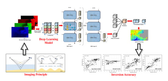
In this paper, a new unified depth inversion framework is proposed based on the GRU model by using the GF-1 wide-field view (WFV) data covering the Liaodong Shoal and 1:150,000 scale sea chart depth data. Aiming at the complex sea areas where relatively deep areas and shallow areas coexist, a complex mapping relationship between spectral features of remote sensing image and water depth value in different sections is established. For the relatively deep area, by analyzing the relationship among seabed information, sea surface micro-scale waves, and remote sensing image values, the feasibility of passive optical remote sensing water depth inversion in comparatively deep areas is analyzed. Finally, comparative experiments are designed with the log-linear model, Stumpf model and other traditional methods, the experiments are carried out from the overall and segment aspects, and the correlation analysis and accuracy evaluation are followed.
5. Results and Discussion
5.1. Accuracy Evaluation Method
In this paper, root means square error (RMSE), mean absolute error (MAE), mean relative error (MRE) and determination coefficient (R2) are used to evaluate the accuracy of water depth inversion and to analyze the water depth inversion effect under the inversion strategy. Among them, RMSE, MAE, and MRE are used to evaluate the error between the inversion results and the observed values. The smaller these values, the better the inversion effect. R2 is also known as the fitting index, which, as its name implies, describes how well the inversion model fits the observed values. The range of R2 is [0, 1], and the closer its value is to 1, the more consistent the inversion results are with the true distribution of observed values.
RMSE (root mean square error)
MAE (mean absolute error)
MRE (mean relative error)
In the above three formulas, and are the inverted water depth value and the true water depth value of the th point, respectively, and is the total number of water depth points participating in the accuracy evaluation.
R
2 (determination coefficient)
In the above formula, is the total sum of squares, is the regression sum of squares, and is the error sum of squares.
5.2. Overall Accuracy Evaluation of Underwater Topography
First, from the perspective of the overall water depth, the four accuracy evaluation methods given in
Section 5.1 are applied to evaluate the inversion effect of the four water depth inversion models (log-linear model [
7], Stumpf model [
9], MLP model, GRU model [
33]), root mean square error (RMSE), mean absolute error (MAE), mean relative error (MRE) and determination coefficient (R
2) are obtained, respectively.
As can be seen from
Table 2, GRU models have significantly improved accuracy when compared with semi-theoretical and semi-empirical models such as the four-band log-linear model and the Stumpf model, as well as MLP statistical models. The RMSE of the GRU model’s inversion results is 3.69 m, the MAE is 2.72 m, and the MRE is 19.6%, indicating a positive inversion effect. For the other three models, the Stumpf model performs the most unsatisfactory in overall inversion, with RMSE of 10.2 m, MAE of 8.1 m, and MRE of 91.6%. Since the four-band log-linear model contains more band information, a slightly better result was achieved in the complex underwater environment of the study area, with three indices of 6.9 m, 5.2 m, and 50.4%, respectively. For the MLP statistical model, the three indices are 6.3 m, 4.8 m, and 30.4%, respectively. It can be seen that compared with the semi-theoretical and semi-empirical model, the statistical model can better deal with problems in complex and diverse environments.
Figure 9 shows the inversion scatter diagram of the four models at the checkpoints, which can more directly judge the inversion effect of these four models. The higher the determination coefficient R
2 is, the more water depth points converge to the standard measurement line, and the better the model fitting is. The lower the determination coefficient, the more divergent the water depth points are to the trend line. As can be seen from the figure, the GRU model has a higher degree of regression than the first three models, with a determination coefficient R
2 of 0.88, while the Stumpf model is 0.16, the four-band log-linear model is 0.60, and the MLP model is 0.69, all of which are significantly lower than the GRU model. It can also be seen from the scatter distribution that the effort of the four-band log-linear model and MLP model in deep water area is relatively poor, and it is difficult to accurately describe the water depth information of areas deeper than 25 m. The Stumpf model is even less satisfactory and can only accurately describe the depth information in the middle depth areas. The GRU model has a concentrated scatter distribution, and the trend line is approximate to the line
, thus obtaining an ideal inversion result.
5.3. Segmented Accuracy Evaluation of Underwater Topography
In the precision analysis of the water division deep section, the errors will be calculated piecewise according to the prediction results of the four models in
Section 5.2. According to the measured water depth, the checkpoints were divided into four groups of segmented point sets, including 0–8 m, 8–16 m, 16–24 m, and 24–32 m, and the MAE and MRE of each model were obtained, respectively. The calculation results are shown in
Figure 10.
It can be seen from the figure that, compared with the semi-theoretical and semi-empirical models and the traditional statistical model, the GRU model has achieved considerable advantages in almost all water depth segments. Only in the depth range of 16–24 m, the Stumpf model gained a small advantage. The performance advantage of the GRU model is especially obvious in the deep (24–32 m) and shallow (0–8 m) areas. In the deep-water area (24–32 m), due to the lack of optical information in the deep area and the small number of water depth samples in this area, the performance of each model is reduced to a certain extent compared with the shallower research areas. However, the GRU still achieves relatively low segmented inversion errors. In the shallow water area (0–8 m), due to the limited global learning ability of other models, especially classical methods, poor inversion results are often obtained. However, the GRU model can still maintain high inversion accuracy in this area, which shows that the GRU model is indeed suitable for the unified inversion work in deep and shallow waters.
5.4. Influence Analysis of Model Parameters
For deep learning methods, the adjustment of the learning rate, batch size, network structure and other hyperparameters usually has a huge influence on the final effect of the model. In this part of the paper, we will carry out comparative experiments from various perspectives and strive to obtain a set of hyperparameter combinations with better effects to provide a model basis for the subsequent overall inversion results. To ensure the fairness and rationality of the experiment, when the comparison experiment is carried out for a certain hyperparameter, the default value of the model or the recommended value of the model will be uniformly used for other hyperparameters.
5.4.1. Network Structure
The differences between different network structures mainly lie in the number of hidden layers and the number of neuron nodes in each layer. This section will carry out comparative experiments and discussions on these two aspects. According to the scale of the problem, 1 to 3 hidden layers are designed for the model, and the specific node number of each hidden layer is shown in
Table 3. The comparison index covers the four accuracy evaluation indices in
Section 5.1 and the training time of the model.
As can be seen from
Table 3, compared with other alternative network structures, the model of double hidden layer structure with 100 and 200 nodes has achieved the best value in multiple evaluation indices, and the model has achieved a good balance between performance and efficiency. Therefore, the network structure will be preferred in the follow-up experiments.
5.4.2. Optimizer Selection
The main work of neural network training is to update parameters and optimize the objective function, so the selection of the optimizer is also an important work affecting the model effect. Common optimizers include SGD, RMSprop, Adagrad, Adadelta, Adam, Adamax, etc. We will carry out comparative experiments with the above six optimizers. The indices of the experimental results are shown in
Table 4, and the MAE variation trends of each model on the validation set are shown in
Figure 11.
It can be seen that after a certain number of iterations, the optimizer Adam achieves the optimal inversion effect by considering the regression accuracy of the model and the stability of the training process. Therefore, this optimizer will be preferred in the following experiments.
5.4.3. Batch Size
Batch-size is the number of samples sent into the model during each round of neural network training. A larger batch-size can usually make the network converge faster, but too large a batch-size will consume many memory resources and require more iterations to meet the model training, so we need to select a suitable size of batch-size for training. We respectively select different numbers as batch-size to carry out the comparison experiment, and the indices of the experimental results are shown in
Table 5.
As can be seen from the above table that in this depth inversion work, when batch-size is set to 64, the model achieves the best efficiency and performance. Therefore, in the follow-up experiments, batch-size will be preferred to take this value.
5.4.4. Number of Iterations
The number of iterations refers to the number of times that the entire training set is input into the neural network for training. Usually, sufficient iterations are required to enable the model to fully learn the information in the training data and to fully build the deep learning model. However, this does not mean that the more iterations, the better. Too many iterations will cause the model to overlearn the information of training data, resulting in the phenomenon of “overfitting” and leads to an increase of the error on the test set.
For this reason, we carried out comparison experiments with different iteration times, and the model structure we use is the 100–200 double hidden layer network structure recommended in
Section 5.4.1. The inversion accuracy of the model at control points and check points are calculated, respectively, and the results are shown in
Figure 12. It can be seen that when the number of iterations is between 2000 and 2500, the MAE curves of the training set and the test set intersect once. When the number of iterations reaches about 2500, the MRE of the training set and the test set is the same. Continuous training will further reduce the MAE and MRE of the training set, but will not reduce the errors of the test set. The model was overfitted to the training data at this time. Therefore, for the model of 100–200 double hidden layer network structure, it is a good choice to choose the number of iterations between 2000 and 2500.
5.5. Influence of Control Points Proportion
For common deep learning problems, to train a model as complete as possible, we usually want the training set to be as rich as possible, including massive training data and high data dimensions. However, for the water depth optical inversion problem, it is difficult to obtain large training data due to the objective difficulties in acquiring the depth control points, which poses a challenge to the usability of the model under the condition of limited samples.
To this end, we carried out experiments by adjusting the proportion of water depth control points. On the premise of maintaining the same other conditions, the proportion of the control points is taken as 10%, 20%, 40%, 60%, 80% to experiment, respectively, and the experimental results are shown in
Table 6. It can be seen that for the problem in this paper with 580 water depth points, as the scale of the control points gradually increases, the evaluation indices are all gradually improved, and this improvement process is especially obvious when the proportion of the control points does not exceed 40%. When the proportion 40%, the determination coefficient R
2 is increased to 0.89, MRE is 20.33%, RMSE and MAE are 3.78 m and 2.78 m. However, if the size of the control points set is further improved, the improvement of evaluation indices is relatively limited. It can be seen that 40% control points (232 points) can meet the needs of water depth optical inversion in this area.
5.6. Spatial Analysis of Underwater Topography Inversion by Remote Sensing
Based on the water depth points mentioned in
Section 2.3.4, a GRU neural network model is established and trained. Moreover, the water depth inversion process of the research area mentioned in
Section 2.2 is carried out.
Figure 13 is the inversion map of water depth in the study area of the Liaodong shoal, and the blank part on the right is the land part processed by masking.
From the water depth inversion results, it is obvious that there are several radial tidal ridges in the northern part of the area. With regular distribution and frequent changes in water depth, most of the water depth values are between 15 m and 32 m. The southern area, namely, the Laotieshan Waterway, has a dramatic change in topography. The deepest area is over 30 m-deep, while the shallowest place is only within 10 m-deep. There is obvious relief in this area, and the slope is also large. The local slope can reach 1–4‰. The results of this bathymetric inversion are consistent with the actual seabed topography characteristics in this research area, which also verifies the correctness of this experiment once again.
5.7. Considerations about the Input Data for Model
The application of the unified water depth inversion framework and GRU model in this paper provides a new perspective and method for the passive optical remote sensing water depth inversion. However, there are still some issues that need further discussion in this study:
- (a)
GF-1 satellite is a multi-spectral satellite with a spatial resolution of 16 m and has four optical bands, which cannot make full use of the sequential feature learning ability of the GRU model. If reliable hyperspectral data are introduced to future work, it is believed that better results will be obtained.
- (b)
The Liaodong Shoal area has a relatively high sediment concentration; the sea water is muddy. Considering that some information such as chlorophyll concentration, yellow substance concentration and suspended substance concentration have considerable influence on the bathymetric optical signal, if these factors can be introduced into the future work, it is believed that the inversion performance of this method can be further improved. At the same time, the dimension of input data will be higher and more suitable for deep learning models.
- (c)
The effects of passive optical remote sensing depth inversion are often limited by the quality of control points and check points. Generally, the sources of bathymetric data include sonar measured data and scanning charts, and their accuracy is usually quite different. This makes the source of training sample points, the precision of data acquisition equipment and acquisition process, and the spatial distribution of sample points all worthy of further study.
- (d)
Deep learning is a data-driven model method. To ensure the learning effect of the deep model, abundant and diverse training data are required in the training process. However, in the water depth inversion work, the lack of sufficient samples is very common. “few shot learning” and “transfer learning” may provide solutions and research directions for this problem.
- (e)
The water depth control points are the basis of building the model, and their quality is very important. In the real scene, the image pixels corresponding to the water depth points in the sea chart are affected by the surface flare and the boundary of the aquaculture area, resulting in the distortion of the pixel spectrum of the remote sensing image, and the predicted values of these pixels are greatly different from the measured values. In fact, these pixels have been “polluted” and are no longer suitable as control points. It should be pointed out that the GRU model also pays attention to the number of control points, and maintaining a certain number of control points is the premise of training an effective model. In this paper, a total of 596 control points was collected. For the points with more than one standard deviation, we carried out a visual interpretation to ensure that they were “polluted” pixels, and 16 points were deleted, and 97% of the points were retained. Therefore, on the premise of ensuring the quality of water depth control points, the quantity of control points is also guaranteed.
6. Conclusions
Based on GF-1 satellite remote sensing data, this paper proposed a unified remote sensing inversion framework for water depth in a composite environment, applied and adjusted a GRU deep learning model to carry out a water depth inversion experiment in the Liaodong Shoal. The main work and conclusions are as follows:
Based on the traditional passive optical inversion principle of shallow water depth, combining with the relationship between underwater topography, flowing water under the sea surface, distribution of the sea surface micro-scale wave, and local flare brightness in non-flare area, this paper analyses the mechanism of passive optical remote sensing inversion in turbid or deep-sea area, and proposes a new inversion framework for water depth, which can simultaneously satisfy the requirements of optical remote sensing depth inversion for shallow and deep areas.
The overall and segmented water depth inversion effects were evaluated, respectively. Through the comparative analysis of various indices, it is found that the GRU model has achieved leading results compared with other traditional inversion methods, both in terms of the overall inversion effect and the local inversion performance in each depth segment. Around the research area of Liaodong Shoal with a complex environment, the model optimization and result analysis are carried out in many aspects. For this research area, the (100–200) double-hidden layer network structure is applied, the Adam optimizer is called to optimize the model, the batch-size is determined to be 64, the training iterations from 2000 to 2500 are used, and determine that at least 40% of sample points can meet the needs of model training.


