What Can Multifractal Analysis Tell Us about Hyperspectral Imagery?

 , , , and
Abstract
:1. Introduction
1.1. Fractals
1.2. Multifractals
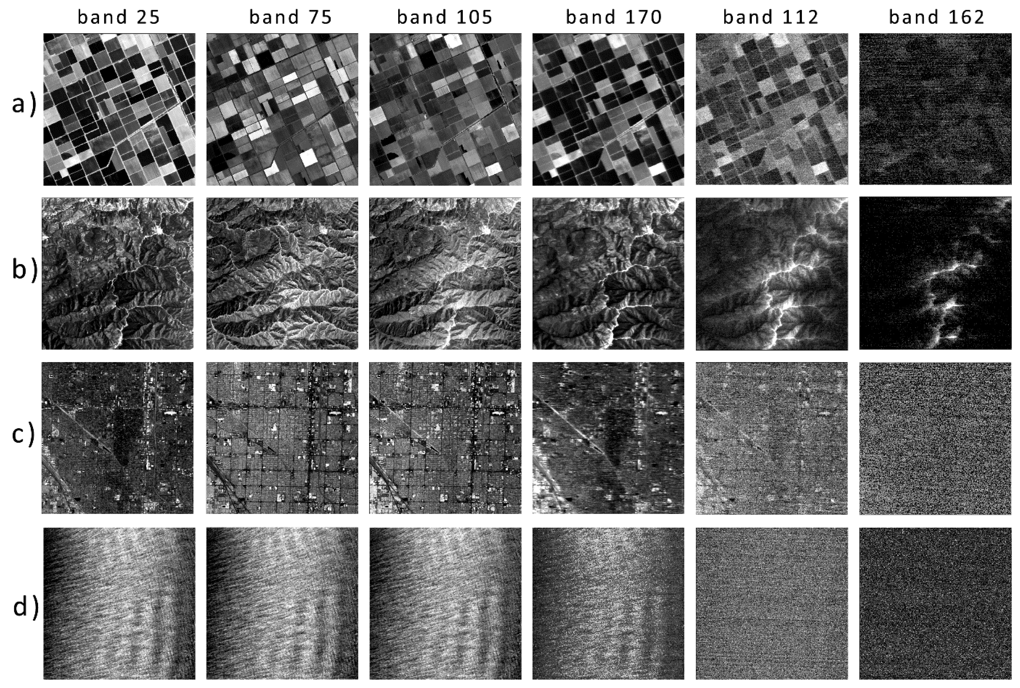
2. Data
3. Methodology
4. Results
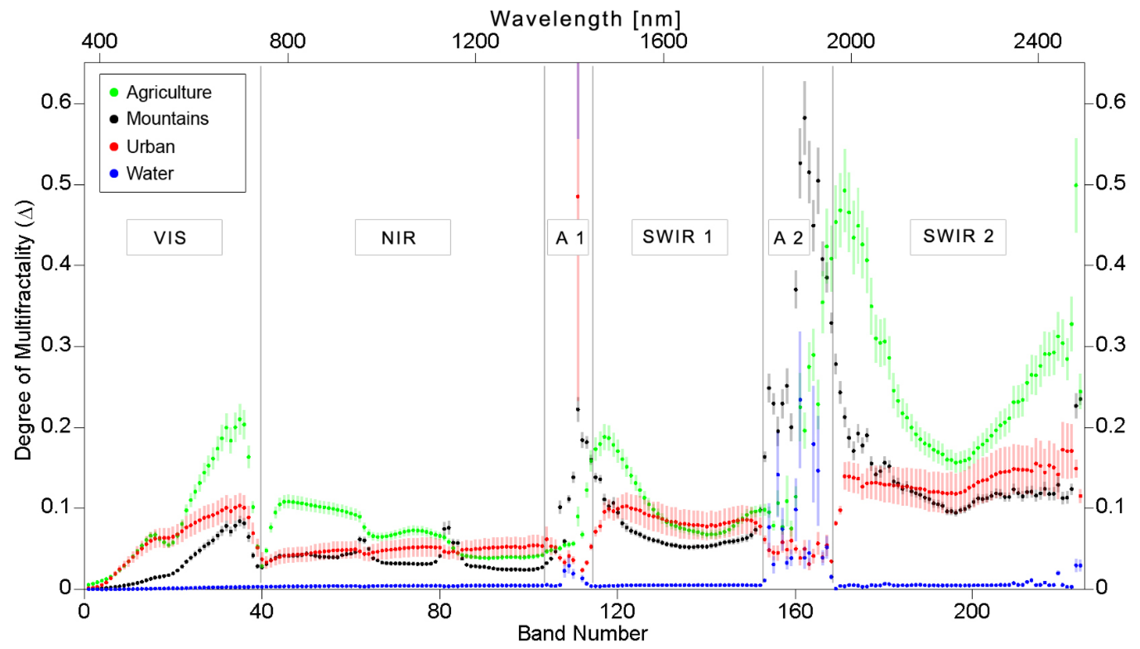
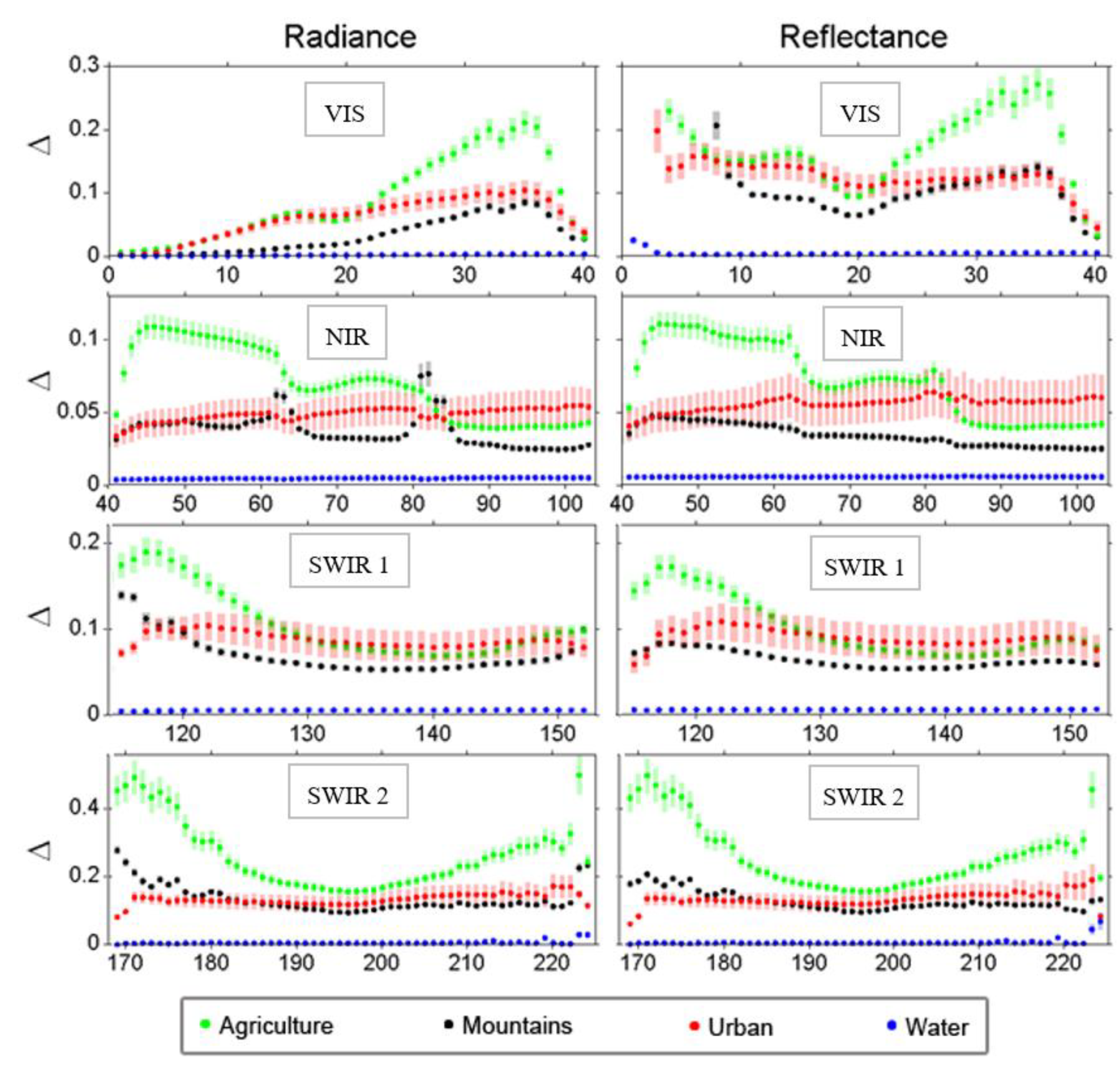
4.1. Degree of Multifractality for Radiance
4.2. Degree of Multifractality for Reflectance
5. Discussion
5.1. Interpretation of the Multifractal Results
5.1.1. Influence of Atmospheric Absorption
5.1.2. Landscape Types and Dimensionality Reduction
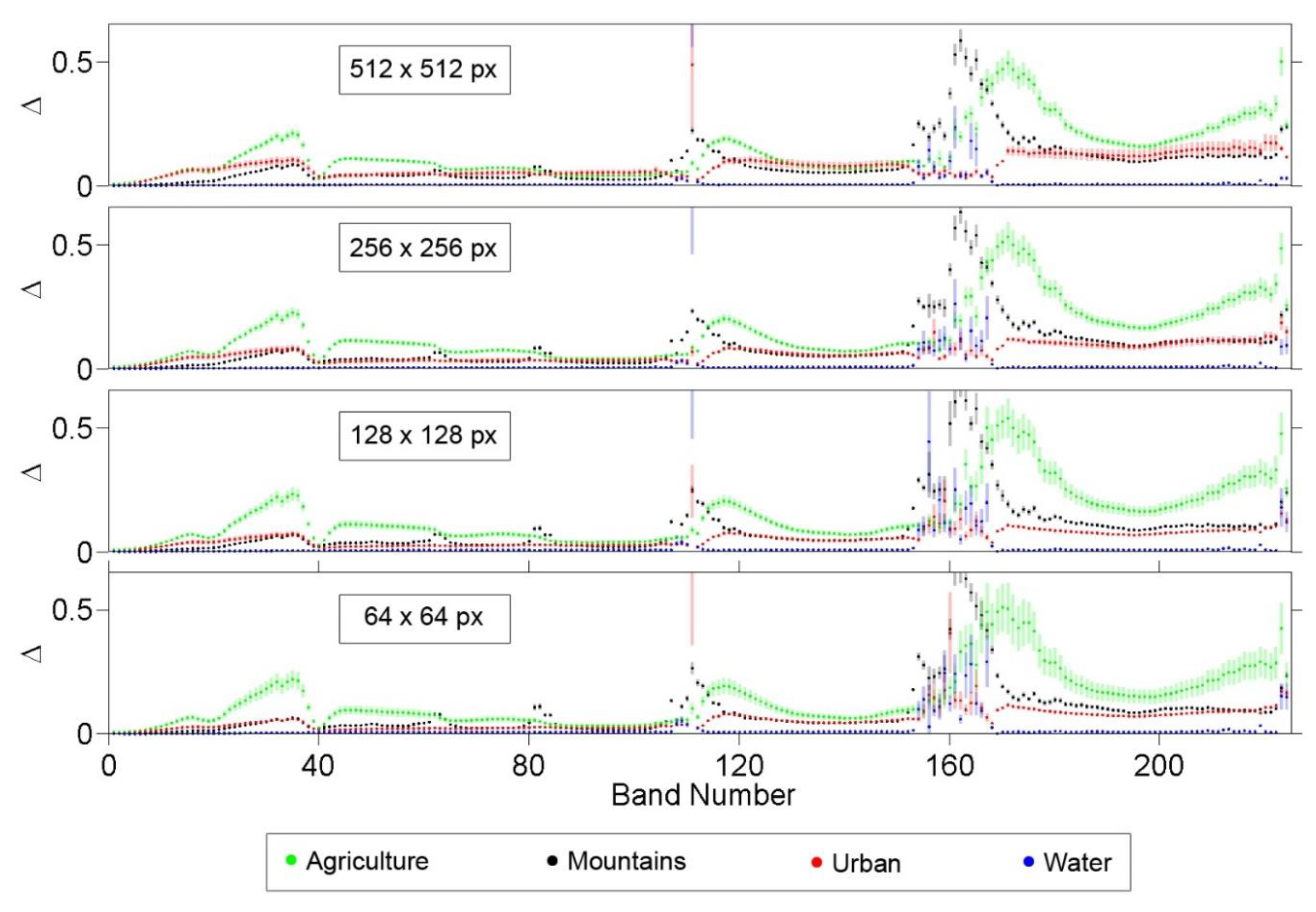
5.1.3. Size of Images and Spatial Resolution
5.2. Comparison with Other Characteristics
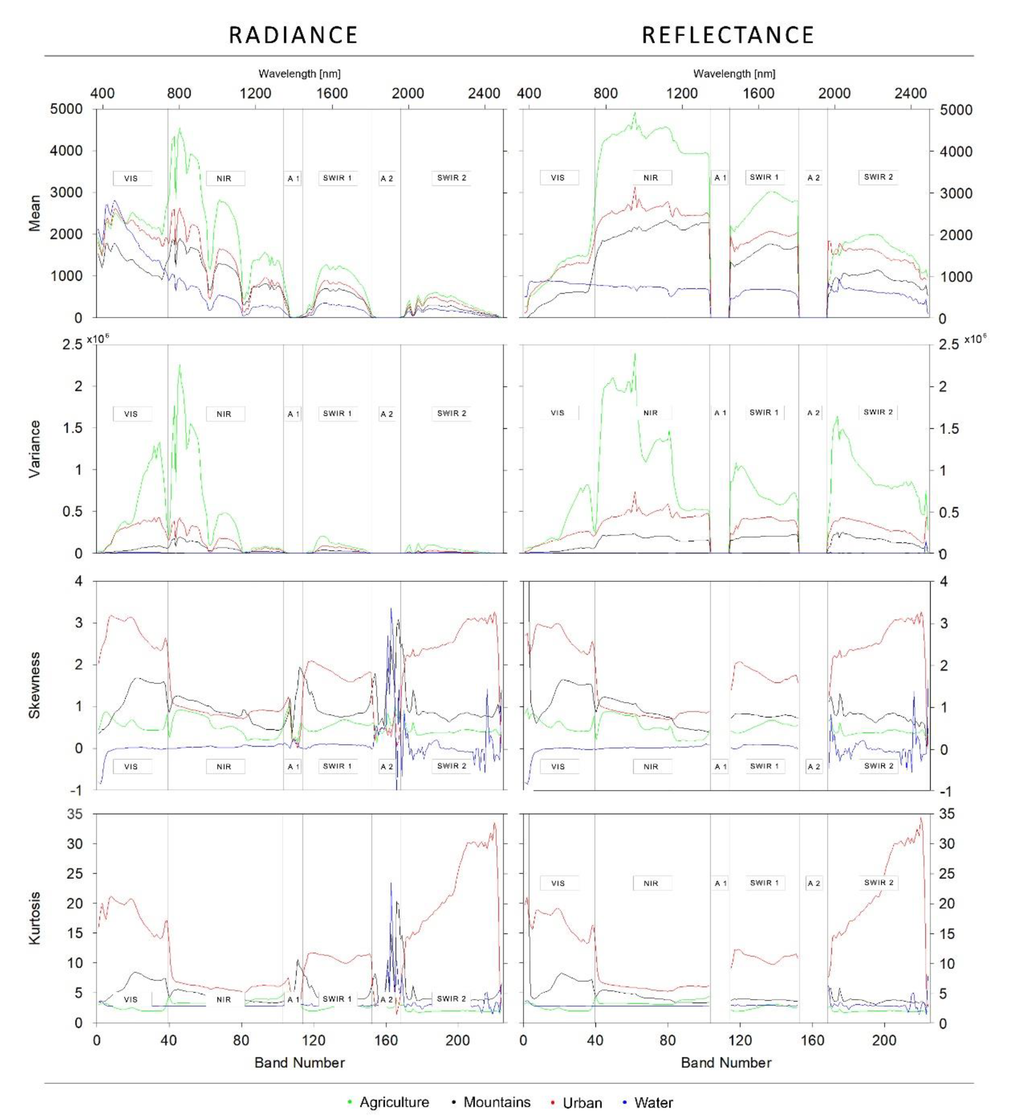
5.2.1. Correlation with Statistical Moments
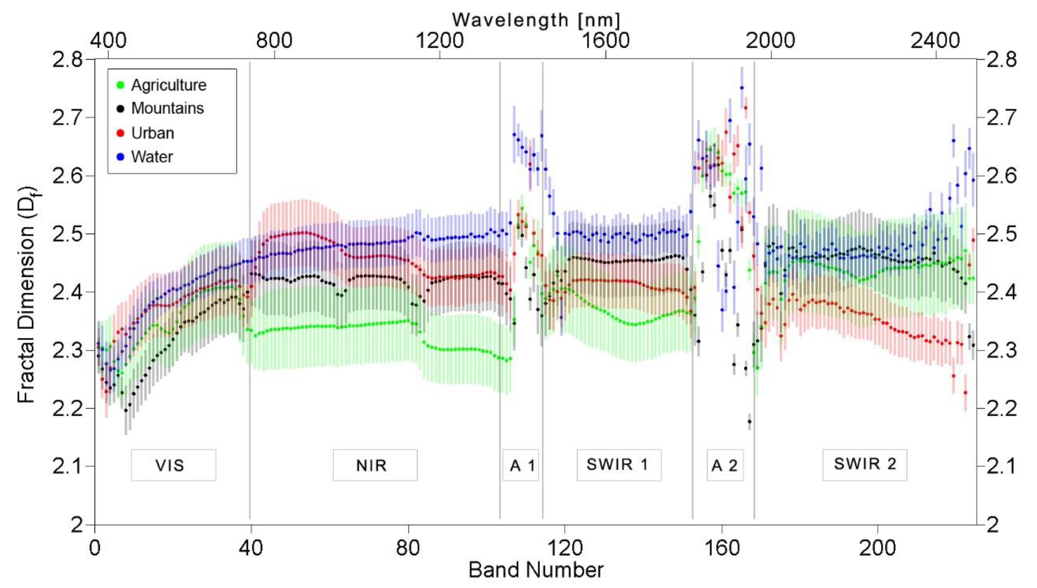
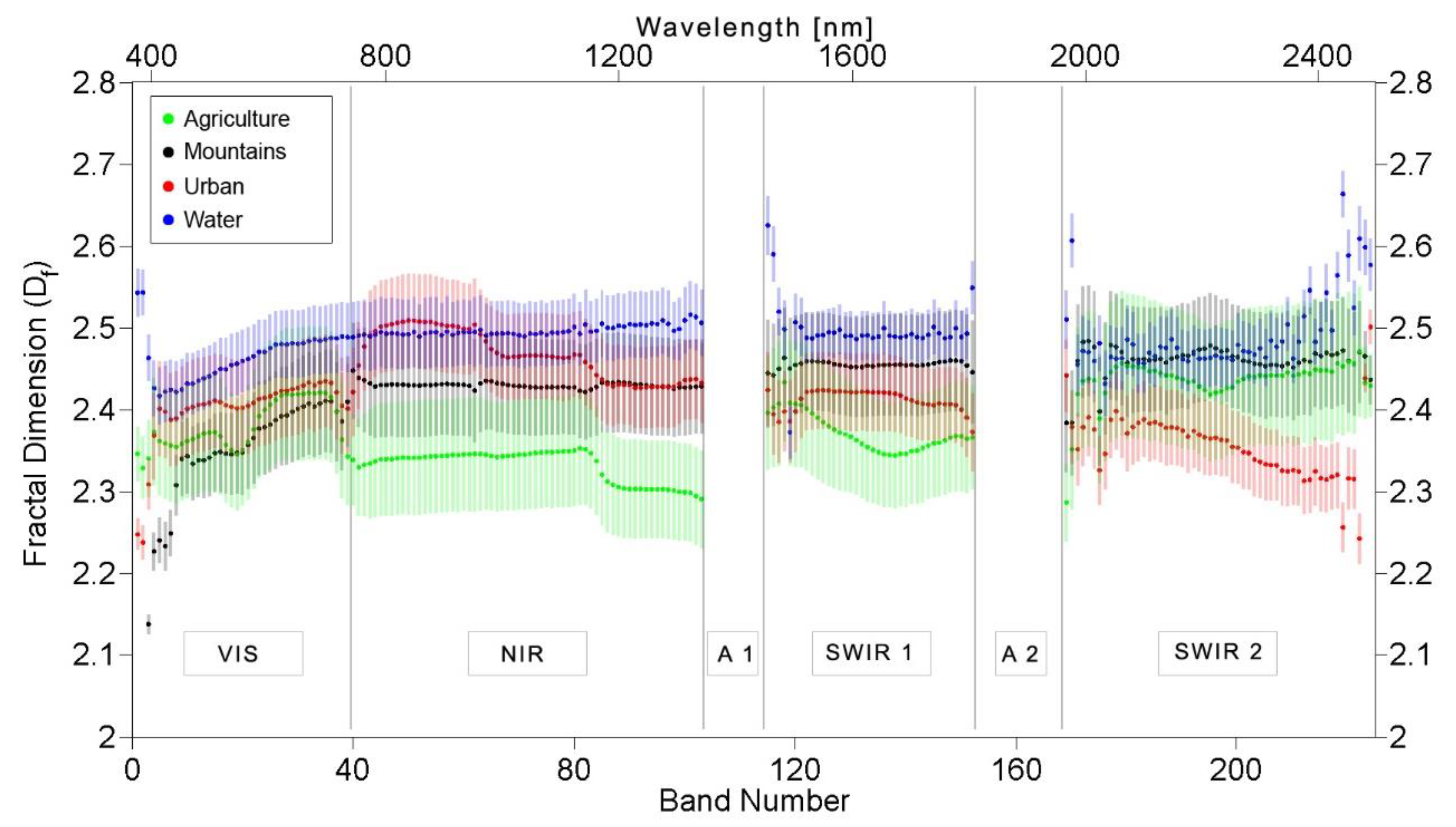
5.2.2. Comparison with Fractal Dimension
6. Conclusions
Author Contributions
Funding
Acknowledgments
Conflicts of Interest
Appendix A

| Landscape Type | Original Image (Radiance) | Original Image (Reflectance) |
|---|---|---|
| Agriculture | f130522t01p00r11rdn_e | f130522t01p00r11_refl |
| Mountains | f130522t01p00r12rdn_e | f130522t01p00r12_refl |
| Urban | f130612t01p00r11rdn_e | f130612t01p00r11_refl |
| Water | f130606t01p00r10rdn_e | f130606t01p00r10_refl |

Appendix B
| Radiance | Reflectance | ||||||||||||
|---|---|---|---|---|---|---|---|---|---|---|---|---|---|
| VIS | NIR | A 1 | SWIR 1 | A 2 | SWIR 2 | All | VIS | NIR | SWIR 1 | SWIR 2 | All | ||
| Agriculture | Min | 0.006 | 0.039 | 0.047 | 0.068 | 0.075 | 0.157 | 0.006 | 0.032 | 0.039 | 0.068 | 0.157 | 0.032 |
| Mean | 0.088 | 0.070 | 0.073 | 0.106 | 0.197 | 0.264 | 0.137 | 0.151 | 0.072 | 0.101 | 0.262 | 0.151 | |
| Max | 0.210 | 0.109 | 0.159 | 0.188 | 0.423 | 0.498 | 0.498 | 0.497 | 0.110 | 0.171 | 0.497 | 0.497 | |
| Mountains | Min | 0.001 | 0.024 | 0.033 | 0.052 | 0.164 | 0.095 | 0.001 | 0.031 | 0.025 | 0.053 | 0.096 | 0.025 |
| Mean | 0.031 | 0.037 | 0.116 | 0.070 | 0.349 | 0.135 | 0.092 | 0.100 | 0.034 | 0.064 | 0.129 | 0.079 | |
| Max | 0.084 | 0.076 | 0.222 | 0.138 | 0.581 | 0.278 | 0.581 | 0.206 | 0.047 | 0.083 | 0.208 | 0.208 | |
| Urban | Min | 0.002 | 0.034 | 0.024 | 0.071 | 0.032 | 0.082 | 0.002 | 0.045 | 0.041 | 0.058 | 0.061 | 0.041 |
| Mean | 0.060 | 0.048 | 0.083 | 0.087 | 0.048 | 0.134 | 0.080 | 0.126 | 0.056 | 0.089 | 0.134 | 0.098 | |
| Max | 0.104 | 0.055 | 0.484 | 0.103 | 0.062 | 0.172 | 0.484 | 0.198 | 0.064 | 0.108 | 0.176 | 0.198 | |
| Water | Min | 0.0003 | 0.004 | 0.004 | 0.004 | 0.011 | 0.001 | 0.0003 | 0.003 | 0.005 | 0.005 | 0.002 | 0.002 |
| Mean | 0.002 | 0.005 | 0.081 | 0.005 | 0.079 | 0.007 | 0.014 | 0.005 | 0.006 | 0.006 | 0.006 | 0.006 | |
| Max | 0.004 | 0.005 | 0.768 | 0.006 | 0.234 | 0.030 | 0.768 | 0.025 | 0.006 | 0.006 | 0.022 | 0.025 | |
| VIS | NIR | A 1 | SWIR 1 | A 2 | SWIR 2 | All | ||
|---|---|---|---|---|---|---|---|---|
| Agriculture | Min | 0.0004 4% | 0.0031 8% | 0.0036 7% | 0.0051 7% | 0.0060 7% | 0.0125 8% | 0.0004 4% |
| Mean | 0.0070 7% | 0.0056 8% | 0.0061 8% | 0.0083 8% | 0.0240 13% | 0.0245 9% | 0.0124 8% | |
| Max | 0.0192 9% | 0.0086 8% | 0.0132 13% | 0.0161 9% | 0.0464 29% | 0.0581 12% | 0.0581 29% | |
| Mountains | Min | 0.0001 5% | 0.0008 2% | 0.0009 2% | 0.0034 4% | 0.0065 4% | 0.0047 3% | 0.0001 2% |
| Mean | 0.0026 9% | 0.0027 7% | 0.0061 5% | 0.0044 6% | 0.0244 7% | 0.0075 6% | 0.0059 7% | |
| Max | 0.0068 15% | 0.0087 11% | 0.0150 8% | 0.0071 8% | 0.0458 9% | 0.0156 7% | 0.0458 15% | |
| Urban | Min | 0.0001 8% | 0.0080 18% | 0.0030 8% | 0.0062 9% | 0.0012 4% | 0.0031 4% | 0.0001 4% |
| Mean | 0.0104 17% | 0.0108 22% | 0.0292 19% | 0.0163 19% | 0.0096 20% | 0.0247 18% | 0.0160 19% | |
| Max | 0.0158 24% | 0.0131 24% | 0.2524 52% | 0.0185 23% | 0.0167 28% | 0.0347 22% | 0.2524 52% | |
| Water | Min | 0.0000 17% | 0.0006 16% | 0.0006 14% | 0.0005 13% | 0.0021 19% | 0.0001 10% | 0.0000 10% |
| Mean | 0.0003 17% | 0.0008 17% | 0.0224 24% | 0.0009 16% | 0.0288 33% | 0.0012 17% | 0.0039 18% | |
| Max | 0.0006 23% | 0.0008 17% | 0.2124 34% | 0.0009 17% | 0.0846 46% | 0.0083 28% | 0.2124 46% | |
| All | Mean | 0.0052 13% | 0.0050 14% | 0.0159 14% | 0.0075 12% | 0.0217 18% | 0.0145 12% |
| Landscape Type | VIS | NIR | SWIR 1 | SWIR 2 |
|---|---|---|---|---|
| Agriculture | 0.007 | 0.0003 | 0.001 | 0.001 |
| 304% | 5% | 5% | 2% | |
| Mountains | 0.004 | 0.001 | 0.001 | 0.001 |
| 542% | 32% | 12% | 7% | |
| Urban | 0.009 | 0.003 | 0.003 | 0.002 |
| 494% | 32% | 21% | 6% | |
| Water | 0.001 | 0.0002 | 0.0001 | 0.00005 |
| 440% | 25% | 11% | 6% | |
| All | 0.005 | 0.001 | 0.001 | 0.001 |
| 442% | 21% | 12% | 5% |
Appendix C
References
- Mandelbrot, B.B. Fractals: Form, Chance, and Dimension; W.H. Freeman & Company: San Francisco, CA, USA, 1977; ISBN 0716704730. [Google Scholar]
- Mandelbrot, B.B. The Fractal Geometry of Nature; Einaudi Paperbacks; Henry Holt and Company: New York, NY, USA, 1983; ISBN 9780716711865. [Google Scholar]
- Chaudhuri, B.B.; Sarkar, N. Texture Segmentation Using Fractal Dimension. IEEE Trans. Pattern Anal. Mach. Intell. 1995, 17, 72–77. [Google Scholar] [CrossRef]
- Gao, Q.; Zribi, M.; Escorihuela, J.M.; Baghdadi, N.; Segui, Q.P. Irrigation Mapping Using Sentinel-1 Time Series at Field Scale. Remote Sens. 2018, 10, 1495. [Google Scholar] [CrossRef] [Green Version]
- Di Martino, G.; Di Simone, A.; Riccio, D. Fractal-Based Local Range Slope Estimation from Single SAR Image with Applications to SAR Despeckling and Topographic Mapping. Remote Sens. 2018, 10, 1294. [Google Scholar] [CrossRef] [Green Version]
- Di Martino, G.; Iodice, A.; Riccio, D.; Ruello, G.; Zinno, I. The Role of Resolution in the Estimation of Fractal Dimension Maps From SAR Data. Remote Sens. 2018, 10, 9. [Google Scholar] [CrossRef] [Green Version]
- Zhou, Y.; Lin, C.; Wang, S.; Liu, W.; Tian, Y. Estimation of Building Density with the Integrated Use of GF-1 PMS and Radarsat-2 Data. Remote Sens. 2016, 8, 969. [Google Scholar] [CrossRef] [Green Version]
- Chen, Q.; Li, L.; Xu, Q.; Yang, S.; Shi, X.; Liu, X. Multi-Feature Segmentation for High-Resolution Polarimetric SAR Data Based on Fractal Net Evolution Approach. Remote Sens. 2017, 9, 570. [Google Scholar] [CrossRef] [Green Version]
- Peleg, S.; Naor, J.; Hartley, R.; Avnir, D. Multiple Resolution Texture Analysis and Classification. IEEE Trans. Pattern Anal. Mach. Intell. 1984, PAMI-6, 518–523. [Google Scholar] [CrossRef] [Green Version]
- Clarke, K.C. Computation of the Fractal Dimension of Topographic Surfaces Using the Triangular Prism Surface Area Method. Comput. Geosci. 1986, 12, 713–722. [Google Scholar] [CrossRef]
- Lam, N.S.N.; De Cola, L. Fractals in Geography; Prentice Hall: Upper Saddle River, NJ, USA, 1993; ISBN 9780131058675. [Google Scholar]
- Sevcik, C. A Procedure to Estimate the Fractal Dimension of Waveforms. Complex. Int. 1998, 5, 1–19. [Google Scholar]
- Turcotte, D.L. Fractals and Chaos in Geology and Geophysics, 2nd ed.; Cambridge University Press: Cambridge, UK, 1997. [Google Scholar]
- Mukherjee, K.; Ghosh, J.K.; Mittal, R.C. Variogram Fractal Dimension Based Features for Hyperspectral Data Dimensionality Reduction. J. Indian Soc. Remote Sens. 2013, 41, 249–258. [Google Scholar] [CrossRef]
- Ghosh, J.K.; Somvanshi, A. Fractal-based Dimensionality Reduction of Hyperspectral Images. J. Indian Soc. Remote Sens. 2008, 36, 235–241. [Google Scholar] [CrossRef]
- Aleksandrowicz, S.; Wawrzaszek, A.; Drzewiecki, W.; Krupinski, M. Change Detection Using Global and Local Multifractal Description. IEEE Geosci. Remote Sens. Lett. 2016, 13, 1183–1187. [Google Scholar] [CrossRef]
- Dong, P. Fractal Signatures for Multiscale Processing of Hyperspectral Image Data. Adv. Space Res. 2008, 41, 1733–1743. [Google Scholar] [CrossRef]
- Mukherjee, K.; Bhattacharya, A.; Ghosh, J.K.; Arora, M.K. Comparative Performance of Fractal Based and Conventional Methods for Dimensionality Reduction of Hyperspectral Data. Opt. Lasers Eng. 2014, 55, 267–274. [Google Scholar] [CrossRef]
- Mukherjee, K.; Ghosh, J.K.; Mittal, R.C. Dimensionality Reduction of Hyperspectral Data Using Spectra Fractal Feature. Geocarto Int. 2012, 27, 515–531. [Google Scholar] [CrossRef]
- Qiu, H.-I.; Lam, N.; Quattrochi, D.; Gamon, J. Fractal Characterization of Hyperspectral Imagery. Photogramm. Eng. Remote Sens. 1999, 65, 63–71. [Google Scholar]
- Myint, S.W. Fractal Approaches in Texture Analysis and Classification of Remotely Sensed Data: Comparison with Spatial Autocorrelation Techniques and Simple Descriptive Statistics. Int. J. Remote Sens. 2003, 24, 1925–1947. [Google Scholar] [CrossRef]
- Krupinski, M.; Wawrzaszek, A.; Drzewiecki, W.; Aleksandrowicz, S. Usefulness of the Fractal Dimension in the Context of Hyperspectral Data Description. In Proceedings of the 14th SGEM GeoConference on Informatics, Geoinformatics and Remote Sensing; STEF92 Technology, Albena, Bulgaria, 17–26 June 2014; Volume 3, pp. 367–374. [Google Scholar] [CrossRef]
- Sarkar, N.; Chaudhuri, B.B. An efficient differential box-counting approach to compute fractal dimension of image. IEEE Trans. Syst. Man Cybern. 1994, 24, 115–120. [Google Scholar] [CrossRef] [Green Version]
- Sun, W.; Xu, G.; Gong, P.; Liang, S. Fractal analysis of remotely sensed images: A review of methods and applications. Int. J. Remote Sens. 2006, 27, 4963–4990. [Google Scholar] [CrossRef]
- Wawrzaszek, A.; Aleksandrowicz, S.; Krupiski, M.; Drzewiecki, W. Influence of Image Filtering on Land Cover Classification when using Fractal and Multifractal Features. Photogramm. Fernerkund. Geoinf. 2014, 2014, 101–115. [Google Scholar] [CrossRef]
- Drzewiecki, W.; Wawrzaszek, A.; Krupinski, M.; Aleksandrowicz, S.; Bernat, K. Comparison of selected textural features as global content-based descriptors of VHR satellite image—The EROS—A study 2013. In Proceedings of the 2013 Federated Conference on Computer Science and Information Systems, Krakow, Poland, 8–11 September 2013; pp. 43–49. [Google Scholar]
- Halsey, T.C.; Jensen, M.H.; Kadanoff, L.P.; Procaccia, I.; Shraiman, B.I. Fractal measures and their singularities: The characterization of strange sets. Nucl. Phys. B Proc. Suppl. 1987, 2, 501–511. [Google Scholar] [CrossRef]
- Hentschel, H.G.E.; Procaccia, I. The infinite number of generalized dimensions of fractals and strange attractors. Phys. D Nonlinear Phenom. 1983, 8, 435–444. [Google Scholar] [CrossRef]
- Su, H.; Sheng, Y.; Du, P. A New Band Selection Algorithm for Hyperspectral Data Based on Fractal Dimension. Int. Arch. Photogramm. Remote Sens. Spat. Inf. Sci. Beijing 2008, XXXVII, 279–284. [Google Scholar]
- Combrexelle, S.; Wendt, H.; Tourneret, J.-Y.; Mclaughlin, S.; Abry, P. Hyperspectral Image Analysis Using Multifractal Attributes. In Proceedings of the 7th IEEE Workshop on Hyperspectral Image and SIgnal Processing: Evolution in Remote Sensing (WHISPERS 2015), Tokyo, Japan, 2–5 June 2015; pp. 1–4. [Google Scholar] [CrossRef] [Green Version]
- Aleksandrowicz, S.; Wawrzaszek, A.; Jenerowicz, M.; Drzewiecki, W.; Krupinski, M. Local Multifractal Description of Bi-Temporal VHR Images. In Proceedings of the 2019 10th International Workshop on the Analysis of Multitemporal Remote Sensing Images (MultiTemp), Shanghai, China, 5–7 August 2019; pp. 1–3. [Google Scholar] [CrossRef]
- Grazzini, J.; Turiel, A.; Yahia, H.; Herlin, I.; Rocquencourt, I. Edge-preserving smoothing of high-resolution images with a partial multifractal reconstruction scheme. In Proceedings of the ISPRS 2004—International Society for Photogrammetry and Remote Sensing XXXV, Istambul, Turkey, 12–23 July 2004; pp. 1125–1129. [Google Scholar]
- Hu, M.-G.; Wang, J.-F.; Ge, Y. Super-resolution reconstruction of remote sensing images using multifractal analysis. Sensors 2009, 9, 8669–8683. [Google Scholar] [CrossRef]
- Chen, Z.; Hu, Y.; Zhang, Y. Effects of Compression on Remote Sensing Image Classification Based on Fractal Analysis. IEEE Trans. Geosci. Remote Sens. 2019, 57, 4577–4590. [Google Scholar] [CrossRef]
- Drzewiecki, W.; Wawrzaszek, A.; Aleksandrowicz, S.; Krupinski, M.; Bernat, K. Comparison of selected textural features as global content-based descriptors of VHR satellite image. In Proceedings of the 2013 IEEE International Geoscience and Remote Sensing Symposium—IGARSS, Melbourne, Australia, 21–26 July 2013; pp. 4364–4366. [Google Scholar] [CrossRef]
- Kupidura, P. The Comparison of Different Methods of Texture Analysis for Their Efficacy for Land Use Classification in Satellite Imagery. Remote Sens. 2019, 11, 1233. [Google Scholar] [CrossRef] [Green Version]
- Chen, Q.; Zhao, Z.; Jiang, Q.; Zhou, J.-X.; Tian, Y.; Zeng, S.; Wang, J. Detecting subtle alteration information from ASTER data using a multifractal-based method: A case study from Wuliang Mountain, SW China. Ore Geol. Rev. 2019, 115, 103182. [Google Scholar] [CrossRef]
- Ghosh, J.K.; Somvanshi, A.; Mittal, R.C. Fractal Feature for Classification of Hyperspectral Images of Moffit Field, USA. Curr. Sci. 2008, 94, 356–358. [Google Scholar]
- Junying, S.; Ning, S. A Dimensionality Reduction Algorithm of Hyper Spectral Image Based on Fract Analysis. Int. Arch. Photogramm. Remote Sens. Spat. Inf. Sci. 2008, XXXVII, 297–302. [Google Scholar]
- Ziyong, Z. Multifractal Based Hyperion Hyperspectral Data Mining. In Proceedings of the 2010 Seventh International Conference on Fuzzy Systems and Knowledge Discovery, Yantai, China, 10–12 August 2010; Volume 5, pp. 2109–2113. [Google Scholar]
- Hosseini, A.; Ghassemian, H. Classification of Hyperspectral and Multifractal Images by Using Fractal Dimension of Spectral Response Curve. In Proceedings of the 20th Iranian Conference on Electrical Engineering (ICEE2012), Tehran, Iran, 15–17 May 2012; pp. 1452–1457. [Google Scholar] [CrossRef]
- Li, N.; Zhao, H.; Huang, P.; Jia, G.R.; Bai, X. A novel logistic multi-class supervised classification model based on multi-fractal spectrum parameters for hyperspectral data. Int. J. Comput. Math. 2015, 92, 836–849. [Google Scholar] [CrossRef]
- Wan, X.; Zhao, C.; Wang, Y.; Liu, W. Stacked sparse autoencoder in hyperspectral data classification using spectral-spatial, higher order statistics and multifractal spectrum features. Infrared Phys. Technol. 2017, 86, 77–89. [Google Scholar] [CrossRef]
- Krupiński, M.; Wawrzaszek, A.; Drzewiecki, W.; Aleksandrowicz, S.; Jenerowicz, M. Multifractal Parameters for Spectral Profile Description. In Proceedings of the IGARSS 2019—2019 IEEE International Geoscience and Remote Sensing Symposium, Yokohama, Japan, 28 July–2 August 2019; pp. 1256–1259. [Google Scholar] [CrossRef]
- Jenerowicz, M.; Wawrzaszek, A.; Krupiński, M.; Drzewiecki, W.; Aleksandrowicz, S. Aplicability of Multifractal Features as Descriptors of the Complex Terrain Situation in IDP/Refugee Camps. In Proceedings of the IGARSS 2019—2019 IEEE International Geoscience and Remote Sensing Symposium, Yokohama, Japan, 28 July–2 August 2019; pp. 2662–2665. [Google Scholar] [CrossRef]
- Jenerowicz, M.; Wawrzaszek, A.; Drzewiecki, W.; Krupiński, M.; Aleksandrowicz, S. Multifractality in Humanitarian Applications: A Case Study of Internally Displaced Persons/Refugee Camps. IEEE J. Sel. Top. Appl. Earth Obs. Remote Sens. 2019, 1–8. [Google Scholar] [CrossRef]
- Drzewiecki, W.; Wawrzaszek, A.; Krupiński, M.; Aleksandrowicz, S.; Bernat, K. Applicability of multifractal features as global characteristics of WorldView-2 panchromatic satellite images. Eur. J. Remote Sens. 2016, 49, 809–834. [Google Scholar] [CrossRef] [Green Version]
- Wawrzaszek, A.; Walichnowska, M.; Krupiński, M. Evaluation of degree of multifractality for description of high resolution data aquired by Landsat satellites. Arch. Fotogram. Kartogr. Teledetekcji 2015, 27, 175–184. (In Polish) [Google Scholar] [CrossRef]
- Green, R.O.; Eastwood, M.L.; Sarture, C.M.; Chrien, T.G.; Aronsson, M.; Chippendale, B.J.; Faust, J.A.; Pavri, B.E.; Chovit, C.J.; Solis, M.; et al. Imaging spectroscopy and the Airborne Visible/Infrared Imaging Spectrometer (AVIRIS). Remote Sens. Environ. 1998, 65, 227–248. [Google Scholar] [CrossRef]
- Gao, B.-C.; Heidebrecht, K.B.; Goetz, A.F.H. Derivation of scaled surface reflectances from AVIRIS data. Remote Sens. Environ. 1993, 44, 165–178. [Google Scholar] [CrossRef]
- Gao, B.-C.; Davis, C.O. Development of a line-by-line-based atmosphere removal algorithm for airborne and spaceborne imaging spectrometers. In Proceedings of the Imaging Spectrometry III, San Diego, CA, USA, 31 October 1997; Volume 3118. [Google Scholar]
- Wawrzaszek, A.; Krupinski, M.; Aleksandrowicz, S.; Drzewiecki, W. Fractal and multifractal characteristics of very high resolution satellite images. In Proceedings of the 2013 IEEE International Geoscience and Remote Sensing Symposium—IGARSS, Melbourne, Australia, 21–26 July 2013; pp. 1501–1504. [Google Scholar] [CrossRef]
- Wawrzaszek, A.; Echim, M.; Bruno, R. Multifractal analysis of heliospheric magnetic field fluctuations observed by Ulysses. Astrophys. J. 2019, 876, 153. [Google Scholar] [CrossRef] [Green Version]

| Paper | Sensor/Dataset | Number of Bands | Image Size | Parameters Used/Method | |
|---|---|---|---|---|---|
| Global description | Qiu et al. (1999) [20] | AVIRIS 1/Malibu AVIRIS/LA | 224 224 | 614 × 512 614 × 512 | Fractal Dimension/isarithm method and triangular prism method |
| Myint et al. (2003) [21] | ATLAS (5 classes) | 15 | 17 × 17 33 × 32 65 × 65 | Fractal dimension/isarithm, triangular prism and variogram method | |
| Su et al. (2008) [29] | OMIS 2/Beijing | 64 | 536 × 512 | Fractal dimension/double blanket method | |
| Krupiński et al. (2014) [22] | AVIRIS (4 classes) AVIRIS/Malibu AVIRIS/LA | 224 224 224 | 512 × 512 512 × 512 512 × 512 | Fractal dimension/differential box counting method | |
| Local description | Combrexelle et al. (2015) [30] | Hyspex/Madonna AVIRIS/Moffit Field | 160 224 | 256 × 256 64 × 64 16 × 16 | Coefficients of the polynomial describing multifractal spectrum/wavelet leader multifractal formalism |
| Paper | Sensor/Dataset | No. of Bands | No. of Classes | Parameters Used/Method | |
|---|---|---|---|---|---|
| Spectral Curve Description | Dong et al. (2008) [17] | HYPERION | 138 of 242 | 5 | Fractal dimension/blanket method |
| Ghosh et al. (2008) [15] | AVIRIS/Moffit Field | 224 | 4 | Fractal dimension/adapted Hausdorff metric | |
| Ghosh et al. (2008) [38] | AVIRIS/Moffit Field | 30 128 | 5 | Fractal dimension/adapted Hausdorff metric | |
| Junying et al. (2008) [39] | MAIS 1 OMIS | 176 of 220 | 4 4 | Fractal dimension/step measurement method | |
| Ziyong et al. (2010) [40] | HYPERION | 191 of 210 12 | - | Fractal dimension/modified blanked method | |
| Hosseini et al. (2012) [41] | HYDICE 2/Washington F210 | 191 of 210 12 | 6 9 | Fractal dimension/Hausdorff metric | |
| Mukherjee et al. (2012) [14] | HYDICE AVIRIS/Indian Pine AVIRIS/Cuprite | 188 of 210 200 of 224 197 of 224 | 5 9 of 16 14 | Fractal dimension/power spectrum method | |
| Mukherjee et al. (2013) [19] | HYDICE AVIRIS/Indian Pine AVIRIS/Cuprite | 188 of 210 200 of 224 197 of 224 | 5 9 of 16 14 | Fractal dimension/variogram method | |
| Mukherjee et al. (2014) [18] | AVIRIS/Indian Pine AVIRIS/Cuprite | 200 of 224 197 of 224 | 9 of 16 14 | Fractal dimension/Sevcik’s method, power spectrum method, variogram method | |
| Li et al. (2015) [42] | PHI 3/Fanglu AVIRIS/Indian Pines | 64 200 of 224 | 6 16 | 4 parameters related to multifractal spectrum | |
| Wan et al. (2017) [43] | AVIRIS/Indian Pines AVIRIS/KSC | 200 of 224 176 of 224 | 9 of 16 13 | Holder exponent, multifractal spectrum features | |
| Krupiński et al. (2019) [44] | CASI 4/University of Houston | 144 | 15 | 6 parameters related to multifractal spectrum/multifractal detrended fluctuation analysis |
| Zone Name | VIS | NIR | A 1 | SWIR 1 | A 2 | SWIR 2 |
|---|---|---|---|---|---|---|
| Bands | 1–40 | 41–103 | 104–114 | 115–152 | 153–168 | 169–224 |
| Wavelength (nm) | 366–724 | 734–1313 | 1323–1423 | 1433–1802 | 1811–1937 | 1947–2496 |
| Landscape Type | VIS | NIR | SWIR 1 | SWIR 2 |
|---|---|---|---|---|
| Agriculture | 0.074 | 0.003 | 0.007 | 0.004 |
| 233% | 4% | 4% | 1% | |
| Mountains | 0.062 | 0.005 | 0.004 | 0.009 |
| 524% | 11% | 8% | 5% | |
| Urban | 0.063 | 0.007 | 0.000 | 0.002 |
| 383% | 15% | 5% | 2% | |
| Water | 0.003 | 0.001 | 0.001 | 0.0003 |
| 446% | 25% | 11% | 6% | |
| All | 0.049 | 0.005 | 0.004 | 0.004 |
| 394% | 9% | 7% | 3% |
| Mean Δ Differences | Mean Error Differences | |||||
|---|---|---|---|---|---|---|
| Landscape Type | 256 × 256 | 128 × 128 | 64 × 64 | 256 × 256 | 128 × 128 | 64 × 64 |
| Agriculture | 0.007 | 0.007 | 0.012 | 0.003 | 0.008 | 0.014 |
| 4% | 4% | 10% | 2% | 5% | 11% | |
| Mountains | 0.006 | 0.012 | 0.015 | 0.001 | 0.002 | 0.002 |
| 6% | 14% | 18% | 1% | 2% | 2% | |
| Urban | 0.023 | 0.033 | 0.037 | 0.008 | 0.012 | 0.014 |
| 29% | 44% | 52% | 4% | 7% | 8% | |
| Water | 0.005 | 0.008 | 0.011 | 0.002 | 0.004 | 0.004 |
| 21% | 44% | 76% | 2% | 2% | 5% | |
| All | 0.010 | 0.015 | 0.019 | 0.003 | 0.005 | 0.009 |
| 15% | 26% | 39% | 2% | 3% | 6% | |
| Landscape Type | Mean | Standard Deviation | Skewness | Kurtosis |
|---|---|---|---|---|
| Agriculture | 0.452 | 0.003 | 0.012 | 0.508 |
| Mountains | 0.664 | 0.075 | 0.038 | 0.012 |
| Urban | 0.834 | 0.500 | 0.858 | 0.762 |
| Water | 0.255 | 0.180 | 0.039 | 0.008 |
Publisher’s Note: MDPI stays neutral with regard to jurisdictional claims in published maps and institutional affiliations. |
© 2020 by the authors. Licensee MDPI, Basel, Switzerland. This article is an open access article distributed under the terms and conditions of the Creative Commons Attribution (CC BY) license (http://creativecommons.org/licenses/by/4.0/).
Share and Cite
Krupiński, M.; Wawrzaszek, A.; Drzewiecki, W.; Jenerowicz, M.; Aleksandrowicz, S. What Can Multifractal Analysis Tell Us about Hyperspectral Imagery? Remote Sens. 2020, 12, 4077. https://doi.org/10.3390/rs12244077
Krupiński M, Wawrzaszek A, Drzewiecki W, Jenerowicz M, Aleksandrowicz S. What Can Multifractal Analysis Tell Us about Hyperspectral Imagery? Remote Sensing. 2020; 12(24):4077. https://doi.org/10.3390/rs12244077
Chicago/Turabian StyleKrupiński, Michał, Anna Wawrzaszek, Wojciech Drzewiecki, Małgorzata Jenerowicz, and Sebastian Aleksandrowicz. 2020. "What Can Multifractal Analysis Tell Us about Hyperspectral Imagery?" Remote Sensing 12, no. 24: 4077. https://doi.org/10.3390/rs12244077