A Machine Learning Approach for Mapping Forest Vegetation in Riparian Zones in an Atlantic Biome Environment Using Sentinel-2 Imagery

 , , ,
, , ,  ,
,  , , and
Abstract
:
1. Introduction
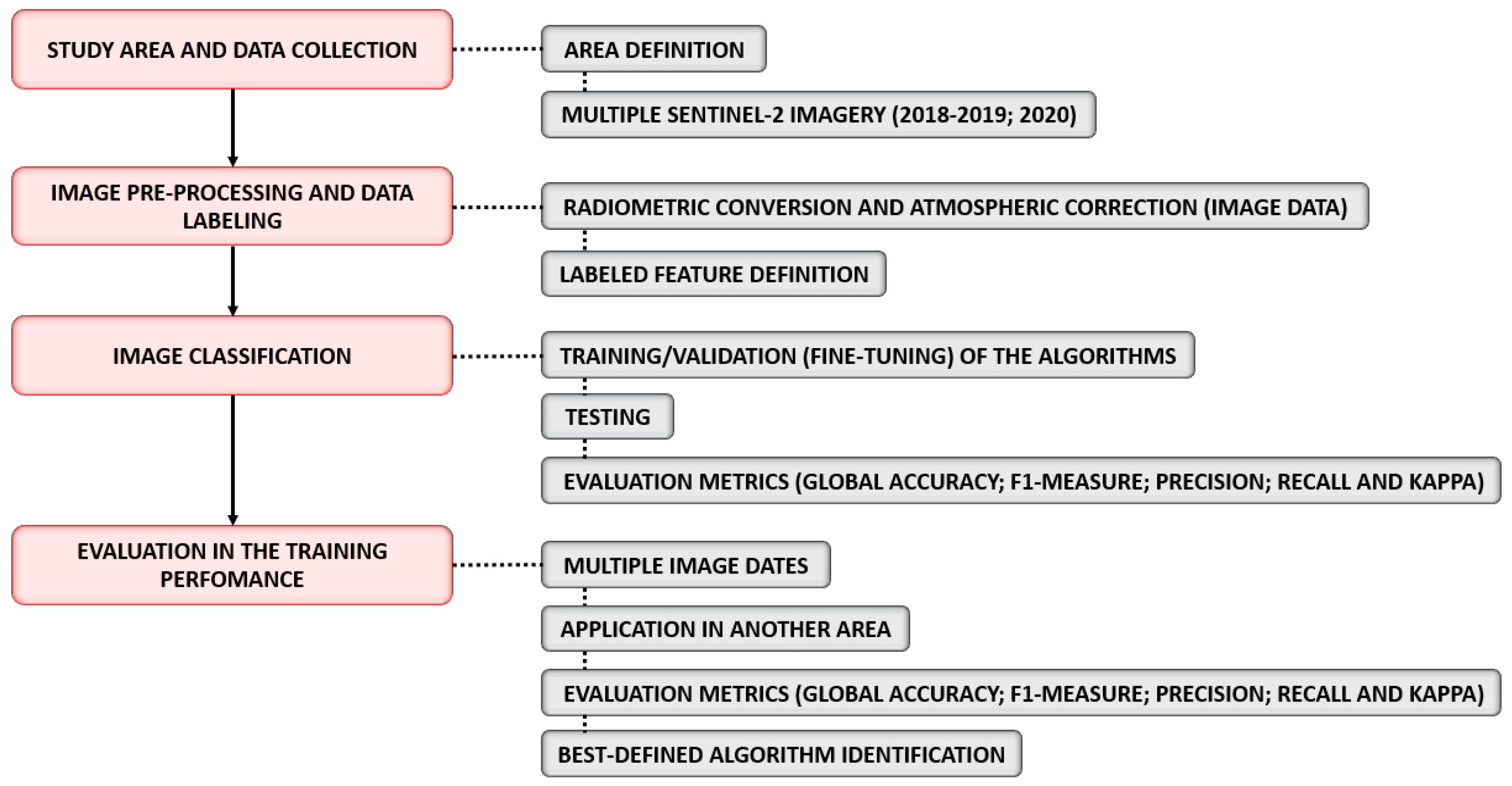
2. Materials and Methods
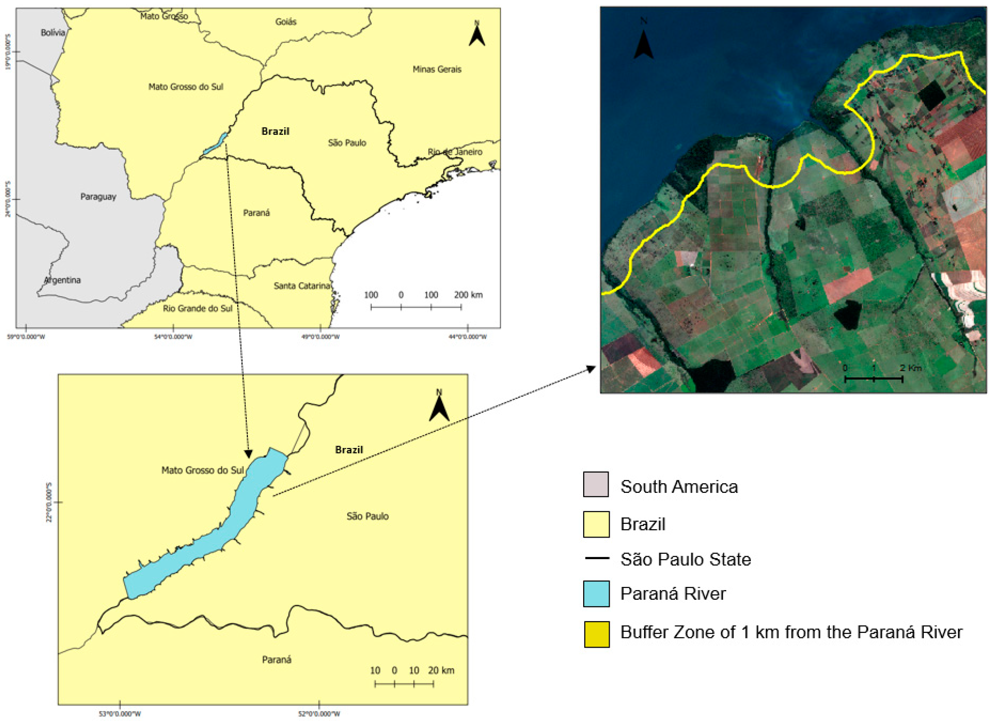
2.1. Study Area
2.2. Image Preprocessing and Labeled Features
2.3. Machine Learning Algorithms
3. Results
4. Discussion
5. Conclusions
Author Contributions
Funding
Acknowledgments
Conflicts of Interest
Appendix A
References
- Midekisa, A.; Holl, F.; Savory, D.J.; Andrade-Pacheco, R.; Gething, P.W.; Bennett, A.; Sturrock, H.J.W. Mapping land cover change over continental Africa using Landsat and Google Earth Engine cloud computing. PLoS ONE 2017, 12, e0184926. [Google Scholar] [CrossRef] [PubMed]
- Chignell, S.M.; Luizza, M.W.; Skach, S.; Young, N.E.; Evangelista, P.H. An integrative modeling approach to mapping wetlands and riparian areas in a heterogeneous Rocky Mountain watershed. Remote Sens. Ecol. Conserv. 2017, 4, 150–165. [Google Scholar] [CrossRef] [Green Version]
- Lawley, V.; Lewis, M.; Clarke, K.; Ostendorf, B. Site-based and remote sensing methods for monitoring indicators of vegetation condition: An Australian review. Ecol. Indic. 2016, 60, 1273–1283. [Google Scholar] [CrossRef] [Green Version]
- Ba, A.; Laslier, M.; Dufour, S.; Hubert-Moy, L. Riparian trees genera identification based on leaf-on/leaf-off airborne laser scanner data and machine learning classifiers in western France. Int. J. Remote Sens. 2019, 41, 1645–1667. [Google Scholar] [CrossRef]
- Jensen, J.R. Remote Sensing of Environment: An Earth Resource Perspective, 2nd ed.; Pearson New International Edition: Harlow, UK, 2014; p. 619. [Google Scholar]
- Richards, J.A. Remote Sensing Digital Image Analysis, 5th ed.; Springer Verlag: New York, NY, USA, 2013; p. 503. [Google Scholar] [CrossRef]
- Ball, J.E.; Anderson, D.T.; Chan, C.S. Comprehensive survey of deep learning in remote sensing: Theories tools and challenges for the community. J. Appl. Remote Sens. 2017, 11, 042609. [Google Scholar] [CrossRef] [Green Version]
- Cheng, X.; Zheng, Y.; Zhang, J.; Yang, Z. Multitask Multisource Deep Correlation Filter for Remote Sensing Data Fusion. IEEE J. Sel. Top. Appl. Earth Obs. Remote Sens. 2020, 13, 3723–3734. [Google Scholar] [CrossRef]
- Mitchell, T.M. Machine Learning, 1st ed.; McGraw-Hill, Inc.: New York, NY, USA, 1997. [Google Scholar]
- Feng, P.; Wang, B.; Liu, D.L.; Yu, Q. Machine learning-based integration of remotely-sensed drought factors can improve the estimation of agricultural drought in South-Eastern Australia. Agric. Syst. 2019, 173, 303–316. [Google Scholar] [CrossRef]
- De Luca, G.; Silva, J.M.N.; Cerasoli, S.; Araújo, J.; Campos, J.; Di Fazio, S.; Modica, G. Object-Based Land Cover Classification of Cork Oak Woodlands using UAV Imagery and Orfeo ToolBox. Remote Sens. 2019, 11, 1238. [Google Scholar] [CrossRef] [Green Version]
- Michez, A.; Piégay, H.; Jonathan, L.; Claessens, H.; Lejeune, P. Mapping of riparian invasive species with supervised classification of Unmanned Aerial System (UAS) imagery. Int. J. Appl. Earth Obs. Geoinf. 2016, 44, 88–94. [Google Scholar] [CrossRef]
- Hengl, T.; Walsh, M.G.; Sanderman, J.; Wheeler, I.; Harrison, S.P.; Prentice, I.C. Global mapping of potential natural vegetation: An assessment of machine learning algorithms for estimating land potential. PeerJ 2018, 6, e5457. [Google Scholar] [CrossRef] [Green Version]
- MacIntyre, P.; Van Niekerk, A.; Mucina, L. Efficacy of multi-season Sentinel-2 imagery for compositional vegetation classification. Int. J. Appl. Earth Obs. 2020, 85, 101980. [Google Scholar] [CrossRef]
- Persson, M.; Lindberg, E.; Reese, H. Tree species classification with multi-temporal Sentinel-2 data. Remote Sens. 2018, 10, 1794. [Google Scholar] [CrossRef] [Green Version]
- Cai, Y.; Zhang, M.; Lin, H. Estimating the Urban Fractional Vegetation Cover Using an Object-Based Mixture Analysis Method and Sentinel-2 MSI Imagery. IEEE J. Sel. Top. Appl. Earth Obs. Remote Sens. 2020, 13, 341–350. [Google Scholar] [CrossRef]
- Feng, S.; Zhao, J.-J.; Liu, T.; Zhang, H.; Zhang, Z.; Guo, X. Crop Type Identification and Mapping Using Machine Learning Algorithms and Sentinel-2 Time Series Data. IEEE J. Sel. Top. Appl. Earth Obs. Remote Sens. 2019, 12, 3295–3306. [Google Scholar] [CrossRef]
- Balcik, F.B.; Senel, G.; Goksel, C. Object-Based Classification of Greenhouses Using Sentinel-2 MSI and SPOT-7 Images: A Case Study from Anamur (Mersin), Turkey. IEEE J. Sel. Top. Appl. Earth Obs. Remote Sens. 2020, 13, 2769–2777. [Google Scholar] [CrossRef]
- Sentinel; European Space Agency (ESA). Sentinel-2 User Handbook; ESA Standard Document; ESA: Paris, France, 2015. Available online: https://sentinels.copernicus.eu/web/sentinel/user-guides/document-library/-/asset_publisher/xlslt4309D5h/content/sentinel-2-user-handbook (accessed on 9 December 2020).
- Maxwell, A.E.; Warner, T.A.; Fang, F. Implementation of machine-learning classification in remote sensing: An applied review. Int. J. Remote Sens. 2018, 39, 2784–2817. [Google Scholar] [CrossRef] [Green Version]
- Breiman, L. Random forests. Mach. Learn. 2001, 45, 5–32. [Google Scholar] [CrossRef] [Green Version]
- Breiman, L.; Friedman, J.H.; Olshen, R.A.; Stone, C.J. Classification and Regression Trees; Chapman and Hall/CRC Press: Boca Raton, FL, USA, 1984. [Google Scholar]
- Mountrakis, G.; Im, J.; Ogole, C. Support vector machines in remote sensing: A review. ISPRS J. Photogramm. Remote Sens. 2011, 66, 247–259. [Google Scholar] [CrossRef]
- Xu, Y.; Goodacre, R. On Splitting Training and Validation Set: A Comparative Study of Cross-Validation, Bootstrap, and Systematic Sampling for Estimating the Generalization Performance of Supervised Learning. J. Anal. Test. 2018, 2, 249–262. [Google Scholar] [CrossRef] [Green Version]
- Sharma, H.; Kumar, S. A survey on decision tree algorithms of classification in data mining. Int. J. Sci. Res. 2016, 5, 2094–2097. [Google Scholar]
- Jadhav, S.D.; Channe, H.P. Comparative Study of K-NN Naive Bayes and Decision Tree Classification Techniques. Int. J. Sci. Res. 2016, 5, 1842–1845. [Google Scholar] [CrossRef]
- Immitzer, M.; Vuolo, F.; Atzberger, C. First experience with sentinel-2 data for crop and tree species classifications in Central Europe. Remote Sens. 2016, 8, 166. [Google Scholar] [CrossRef]
- Brovelli, M.A.; Sun, Y.; Yordanov, V. Monitoring forest change in the amazon using multi-temporal remote sensing data and machine learning classification on Google Earth Engine. ISPRS Int. J. Geo-Inf. 2020, 9, 580. [Google Scholar] [CrossRef]
- Haq, M.A.; Rahaman, G.; Baral, P.; Ghosh, A. Deep Learning Based Supervised Image Classification Using UAV Images for Forest Areas Classification. J. Indian Soc. Remote Sens. 2020, 3, 1–6. [Google Scholar] [CrossRef]
- Sothe, C.; De Almeida, C.M.; Schimalski, M.B.; Liesenberg, V.; La Rosa, L.E.C.; Castro, J.D.B.; Feitosa, R.Q. A comparison of machine and deep-learning algorithms applied to multisource data for a subtropical forest area classification. Int. J. Remote Sens. 2020, 41, 1943–1969. [Google Scholar] [CrossRef]
- Koskikala, J.; Kukkonen, M.; Käyhkö, N. Mapping natural forest remnants with multi-source and multi-temporal remote sensing data for more informed management of global biodiversity hotspots. Remote Sens. 2020, 12, 1429. [Google Scholar] [CrossRef]
- Hamdi, Z.M.; Brandmeier, M.; Straub, C. Forest damage assessment using deep learning on high resolution remote sensing data. Remote Sens. 2019, 11, 1976. [Google Scholar] [CrossRef] [Green Version]
- Rapinel, S.; Mony, C.; Lecoq, L.; Clément, B.; Thomas, A.; Hubert-Moy, L. Evaluation of Sentinel-2 time-series for mapping floodplain grassland plant communities. Remote Sens. Environ. 2019, 223, 115–129. [Google Scholar] [CrossRef]


| Date | Season in the South Hemisphere |
|---|---|
| 20 June 2018 | Autumn |
| 20 July 2018 | Winter |
| 29 August 2018 | Winter |
| 23 September 2018 | Spring |
| 28 October 2018 | Spring |
| 27 November 2018 | Spring |
| 02 December 2018 | Spring |
| 31 January 2019 | Summer |
| 10 February 2019 | Summer |
| 22 March 2019 | Autumn |
| 26 April 2019 | Autumn |
| 21 May 2019 | Autumn |
| 15 June 2019 | Autumn |
| 24 June 2020 | Winter |
| Dataset | Number of Samples (Features—Polygon) | Area (ha) | Number of Pixels |
|---|---|---|---|
| Training (Forest) | 430 | 839.00 | 8,390,000 |
| Training (Non-Forest) | 425 | 679.05 | 6,790,500 |
| Testing (Forest) | 447 | 893.40 | 8,934,000 |
| Testing (Non-Forest) | 408 | 910.85 | 9,108,500 |
| Algorithm | Hyperparameters |
|---|---|
| RF | Maximum depth of the tree = 5 Minimum number of samples in each node = 10 Termination criteria for regression tree = 0 Cluster possible values of a categorical variable into k <= clusters to find a suboptimal split = 10 Size of the randomly selected subset of features at each tree node = 0 Maximum number of trees in the forest = 100 Sufficient accuracy = 0.01 |
| SVM | SVM Kernel Type = Linear SVM Model Type = C support vector classification Cost parameter C = 1 Cost parameter Nu = 0.5 Parameters optimization = Off Probability estimation = Off |
| DT | Maximum depth of the tree = 10 Minimum number of samples in each node = 10 Termination criteria for regression tree = 0.01 Cluster possible values of a categorical variable into k <= cat clusters to find a suboptimal split = 10 |
| NB | The algorithm has no parameters for changing |
| Algorithm—Date | Accuracy (%) | F1-Measure (%) | Precision (%) | Recall (%) | Kappa (%) |
|---|---|---|---|---|---|
| RF—June 2018 | 86.10 | 84.35 | 73.64 | 98.70 | 72.30 |
| RF—July 2018 | 86.10 | 84.35 | 73.64 | 98.70 | 72.30 |
| RF—August 2018 | 96.55 | 89.55 | 82.55 | 96.55 | 75.10 |
| RF—September 2018 | 97.07 | 90.74 | 84.41 | 97.07 | 75.70 |
| RF—October 2018 | 94.79 | 94.60 | 89.89 | 99.84 | 89.60 |
| RF—November 2018 | 93.01 | 92.63 | 86.39 | 99.83 | 86.00 |
| RF—December 2018 | 88.38 | 87.25 | 78.22 | 98.64 | 76.80 |
| RF—January 2019 | 56.29 | 38.67 | 27.10 | 67.44 | 13.40 |
| RF—February 2019 | 80.25 | 76.29 | 62.51 | 97.85 | 60.70 |
| RF—March 2019 | 92.92 | 93.92 | 95.69 | 90.87 | 85.80 |
| RF—April 2019 | 97.13 | 97.19 | 97.90 | 96.50 | 94.20 |
| RF—May 2019 | 86.28 | 85.39 | 78.86 | 93.10 | 72.60 |
| RF—June 2019 | 95.42 | 95.38 | 93.08 | 97.80 | 90.80 |
| RF—June 2020 | 67.48 | 58.22 | 44.57 | 83.91 | 35.50 |
| SVM—June 2018 | 90.38 | 89.62 | 81.76 | 99.16 | 80.80 |
| SVM—July 2018 | 88.02 | 82.77 | 77.52 | 88.02 | 81.55 |
| SVM—August 2018 | 85.25 | 81.67 | 78.10 | 85.25 | 80.77 |
| SVM—September 2018 | 86.39 | 84.59 | 73.48 | 99.65 | 72.90 |
| SVM—October 2018 | 96.79 | 96.76 | 94.19 | 99.46 | 93.60 |
| SVM—November 2018 | 93.60 | 93.46 | 89.89 | 97.32 | 87.20 |
| SVM—December 2018 | 91.89 | 91.70 | 88.18 | 95.52 | 83.80 |
| SVM—January 2019 | 84.61 | 83.21 | 75.03 | 93.39 | 69.30 |
| SVM—February 2019 | 80.93 | 78.30 | 67.68 | 92.89 | 62.00 |
| SVM—March 2019 | 91.27 | 91.74 | 95.32 | 88.41 | 82.50 |
| SVM—April 2019 | 95.81 | 95.90 | 96.46 | 95.35 | 91.60 |
| SVM—May 2019 | 93.03 | 92.87 | 89.37 | 96.66 | 86.10 |
| SVM—June 2019 | 95.87 | 95.92 | 95.50 | 96.33 | 91.70 |
| SVM—June 2020 | 82.94 | 80.08 | 67.47 | 98.48 | 66.00 |
| DT—June 2018 | 92.27 | 92.64 | 95.75 | 89.73 | 84.50 |
| DT—July 2018 | 94.83 | 94.81 | 92.91 | 96.79 | 89.70 |
| DT—August 2018 | 91.72 | 91.49 | 87.58 | 95.76 | 83.50 |
| DT—September 2018 | 92.41 | 92.09 | 86.84 | 98.02 | 84.90 |
| DT—October 2018 | 92.61 | 92.62 | 91.18 | 94.11 | 85.20 |
| DT—November 2018 | 89.25 | 89.22 | 87.49 | 91.02 | 78.50 |
| DT—December 2018 | 87.60 | 87.55 | 85.73 | 89.44 | 75.20 |
| DT—January 2019 | 46.20 | 45.70 | 44.53 | 46.93 | −07.50 |
| DT—February 2019 | 80.78 | 81.17 | 81.50 | 80.84 | 61.50 |
| DT—March 2019 | 91.63 | 92.17 | 96.90 | 87.87 | 83.20 |
| DT—April 2019 | 95.74 | 95.91 | 98.29 | 93.65 | 91.50 |
| DT—May 2019 | 68.26 | 74.77 | 92.50 | 62.74 | 36.00 |
| DT—June 2019 | 97.61 | 97.66 | 97.87 | 97.44 | 95.20 |
| DT—June 2020 | 67.95 | 75.07 | 94.94 | 62.08 | 35.30 |
| NB—June 2018 | 96.74 | 96.71 | 94.45 | 99.09 | 93.50 |
| NB—July 2018 | 94.22 | 93.95 | 93.69 | 94.22 | 91.25 |
| NB—August 2018 | 95.58 | 94.90 | 94.22 | 95.58 | 92.58 |
| NB—September 2018 | 90.49 | 89.69 | 81.35 | 99.93 | 81.00 |
| NB—October 2018 | 78.95 | 81.24 | 89.67 | 74.26 | 57.70 |
| NB—November 2018 | 61.70 | 68.74 | 82.85 | 58.74 | 22.80 |
| NB—December 2018 | 70.93 | 75.41 | 87.70 | 66.14 | 41.50 |
| NB—January 2019 | 76.69 | 78.09 | 81.73 | 74.76 | 53.30 |
| NB—February 2019 | 80.75 | 82.58 | 89.77 | 76.46 | 61.40 |
| NB—March 2019 | 92.88 | 93.24 | 96.55 | 90.15 | 85.70 |
| NB—April 2019 | 96.30 | 96.42 | 97.99 | 94.91 | 92.60 |
| NB—May 2019 | 94.16 | 94.26 | 94.37 | 94.16 | 88.30 |
| NB—June 2019 | 97.62 | 97.66 | 98.04 | 97.29 | 95.20 |
| NB—June 2020 | 86.61 | 87.91 | 95.78 | 81.24 | 73.10 |
| Algorithm—Date | Accuracy (%) | F1-Measure (%) | Precision (%) | Recall (%) | Kappa |
|---|---|---|---|---|---|
| RF—December 2018 | 96.12 | 97.65 | 96.71 | 98.61 | 86.50 |
| RF—June 2019 | 98.67 | 99.21 | 99.57 | 98.85 | 95.10 |
| SVM—December 2018 | 99.08 | 99.44 | 98.92 | 99.98 | 96.70 |
| SVM—June 2019 | 98.68 | 99.21 | 99.81 | 98.62 | 95.10 |
| DT—December 2018 | 95.65 | 97.42 | 98.43 | 96.43 | 83.60 |
| DT—June 2019 | 99.04 | 99.42 | 99.87 | 98.99 | 96.50 |
| NB—December 2018 | 94.39 | 96.71 | 98.88 | 94.63 | 77.70 |
| NB—June 2019 | 98.90 | 99.35 | 99.67 | 99.03 | 96.00 |
Publisher’s Note: MDPI stays neutral with regard to jurisdictional claims in published maps and institutional affiliations. |
© 2020 by the authors. Licensee MDPI, Basel, Switzerland. This article is an open access article distributed under the terms and conditions of the Creative Commons Attribution (CC BY) license (http://creativecommons.org/licenses/by/4.0/).
Share and Cite
Furuya, D.E.G.; Aguiar, J.A.F.; Estrabis, N.V.; Pinheiro, M.M.F.; Furuya, M.T.G.; Pereira, D.R.; Gonçalves, W.N.; Liesenberg, V.; Li, J.; Marcato Junior, J.; et al. A Machine Learning Approach for Mapping Forest Vegetation in Riparian Zones in an Atlantic Biome Environment Using Sentinel-2 Imagery. Remote Sens. 2020, 12, 4086. https://doi.org/10.3390/rs12244086
Furuya DEG, Aguiar JAF, Estrabis NV, Pinheiro MMF, Furuya MTG, Pereira DR, Gonçalves WN, Liesenberg V, Li J, Marcato Junior J, et al. A Machine Learning Approach for Mapping Forest Vegetation in Riparian Zones in an Atlantic Biome Environment Using Sentinel-2 Imagery. Remote Sensing. 2020; 12(24):4086. https://doi.org/10.3390/rs12244086
Chicago/Turabian StyleFuruya, Danielle Elis Garcia, João Alex Floriano Aguiar, Nayara V. Estrabis, Mayara Maezano Faita Pinheiro, Michelle Taís Garcia Furuya, Danillo Roberto Pereira, Wesley Nunes Gonçalves, Veraldo Liesenberg, Jonathan Li, José Marcato Junior, and et al. 2020. "A Machine Learning Approach for Mapping Forest Vegetation in Riparian Zones in an Atlantic Biome Environment Using Sentinel-2 Imagery" Remote Sensing 12, no. 24: 4086. https://doi.org/10.3390/rs12244086
APA StyleFuruya, D. E. G., Aguiar, J. A. F., Estrabis, N. V., Pinheiro, M. M. F., Furuya, M. T. G., Pereira, D. R., Gonçalves, W. N., Liesenberg, V., Li, J., Marcato Junior, J., Prado Osco, L., & Ramos, A. P. M. (2020). A Machine Learning Approach for Mapping Forest Vegetation in Riparian Zones in an Atlantic Biome Environment Using Sentinel-2 Imagery. Remote Sensing, 12(24), 4086. https://doi.org/10.3390/rs12244086