On the Contribution of Satellite Altimetry-Derived Water Surface Elevation to Hydrodynamic Model Calibration in the Han River

Abstract

Satellite altimetry can fill the spatial gaps of in-situ gauging networks especially in poorly gauged regions. Although at a generally low temporal resolution, satellite altimetry has been successfully used for water surface elevation (WSE) estimation and hydrodynamic modeling. This study aims to investigate the contribution of WSE from both short-repeat and geodetic altimetry to hydrodynamic model calibration, and also explore the contribution of the new Sentinel-3 mission. Two types of data sources (i.e., in-situ and satellite altimetry) are investigated together with two roughness cases (i.e., spatially variable and uniform roughness) for calibration of a hydrodynamic model (DHI MIKE 11) with available bathymetry. A 150 km long reach of Han River in China with rich altimetry and in-situ gauging data is selected as a case study. Results show that the performances of the model calibrated by satellite altimetry-derived datasets are acceptable in terms of Root Mean Square Error (RMSE) of simulated WSE. Sentinel-3A can support hydrodynamic model calibration even though it has a relatively low temporal resolution (27-day repeat cycle). The CryoSat-2 data with a higher spatial resolution (7.5 km at the Equator) are proved to be more valuable than the Sentinel-3A altimetry data with a low spatial resolution (104 km at the Equator) for hydrodynamic model calibration in terms of RMSE values of 0.16 and 0.18 m, respectively. Moreover, the spatially variable roughness can also improve the model performance compared to the uniform roughness case, with decreasing RMSE values by 2–14%. Our finding shows the value of satellite altimetry-derived datasets for hydrodynamic model calibration and therefore supports flood risk assessment and water resources management.

1. Introduction

Climate change and human activities have altered the river flow regimes and led to more frequent and severe extreme natural disasters, such as floods and droughts [1,2]. Monitoring hydraulic variables and relevant hydrological-hydraulic processes of rivers usually play an essential role in flood risk assessment and water resources management [3,4]. One of the key hydraulic variables is the water surface elevation (WSE), which refers to the height of surface water above a given datum (i.e., 1985 National Height Datum of China for in-situ records, and EGM2008 datum for satellite WSE) [5]. Reliable and timely estimation of WSE is important for flood and water resources management tasks [6,7]. Traditionally, WSE measurements relied on in-situ gauging stations and often suffered from insufficient spatial coverage and data access constraints [8,9]. Hydraulic infrastructure and engineering projects are often designed in data sparsely or ungauged river reaches, which hampers the stakeholders to make decisions about river system management [10]. Hence, it is difficult for engineers to find an efficient way for WSE estimation along the entire river reach. Currently, a practical way to achieve this goal is the comprehensive estimation of WSE and other hydraulic variables on a whole river reach by using hydrodynamic models [4,11].

A hydrodynamic model is an efficient tool for flood forecasting and water resources management, as it can simulate the spatio-temporal dynamics of hydraulic variables given the boundary and initial conditions [12,13]. Observed data including WSE is often employed to calibrate the parameters of the hydrodynamic model and thus influences the model performance of simulated hydraulic variables [14]. However, observations from in-situ gauging stations are often sparse, and model parameters (e.g., spatially variable roughness parameters) probably cannot be estimated well from in-situ data through a calibration procedure [15]. The hydrodynamic model application is constrained in flood and water resources management, especially in ungauged or poorly gauged basins [16,17,18].

With the rapid advances in remote sensing sciences and technologies, space-borne sensors have provided valuable estimates of hydrological-hydraulic variables such as river extents and WSE [19,20,21,22]. WSE can be freely obtained from satellite altimetry missions (e.g., Envisat and Jason-2/-3), while river extents can be derived from optical or SAR (synthetic aperture radar) imagery satellite missions (e.g., Landsat and Sentinel-1/-2) [23,24]. These data from a satellite mission called satellite observations have been taken as a key supplement to in-situ data for hydrodynamic modeling. There have been many studies focusing on integrating satellite observations in facilitating hydrodynamic modeling. For example, satellite imagery observations have been adopted to calibrate two-dimensional (2-D) hydrodynamic models [25,26], to validate the efficiency of hydrodynamic models [27,28], and even integrated into model structures for data assimilation [29]. Although promising results have been shown by integrating satellite imagery observations in hydrodynamic modeling, there are also a lot of challenges. For example, optical imagery data are easily affected by cloud conditions while SAR imagery data always suffer the low spatial resolution [30], inundation extents are hard to be interpreted due to the noise of the backscatter and are also unavailable during the flood period.

WSE characterizes the surface water variations [31]. Satellite altimetry-derived WSE has been widely used to calibrate hydrodynamic models as an alternative to in-situ records, especially in ungauged areas [32,33]. For example, short-repeat missions such as Envisat and ERS-2 have been adopted in calibrating a quasi-two-dimensional hydrodynamic model in Italy [30]. Recently, CryoSat-2 was used to calibrate a one-dimensional hydrodynamic model in the Brahmaputra River [34].

Hydrodynamic models can benefit from satellite altimetry data in model calibration, improving the skills of simulating hydraulic variables such as WSE and discharge. However, the contributions of various altimetry-derived WSE datasets to hydrodynamic model calibration are different. The data-quality and sampling density are two potential pivotal factors influencing the contribution of satellite WSE on hydrodynamic model calibration. Previous works have revealed the importance of altimetry spatial sampling density to hydrodynamic model calibration through providing a high number of virtual river stage gauging stations from satellite altimetry [35,36], exploring the value of CryoSat-2 altimetry with dense sampling patterns [34], or applying various altimetry-derived datasets to hydrodynamic model calibration [37]. However, few studies have simultaneously evaluated the contributions of WSE from both short-repeat and geodetic altimetry missions on hydrodynamic model calibration, and also little is known about the contribution of the new Sentinel-3 mission [38].

Short-repeat missions such as Sentinel-3 have a repeat cycle of 10 to 35 days with a relatively sparse ground track pattern, while geodetic missions such as CryoSat-2 have dense point observations of the river longitudinal profile due to their drifting ground track pattern [39,40]. As a new generation satellite altimetry mission with a 27-day repeat cycle, Sentinel-3 is likely to deliver high-quality WSE observation for its new open-loop tracking and SAR modes [38]. The CryoSat-2 was launched in July 2010 to an orbit with a 369-day full repeat cycle and dense ground tracks [41]. Sentinel-3 is operating in a constellation of two-satellites (Sentinel-3A and Sentinel-3B). The Sentinel-3A (S3A) and Sentinel-3B (S3B) were launched in February 2016 and April 2018, respectively. Detailed information on Sentinel-3 and CryoSat-2 is available at https://earth.esa.int/web/guest/missions/esa-operational-eo-missions/.

This study aims to investigate the contribution of altimetry-derived WSE from short-repeat and geodetic missions (Sentinel-3A and CryoSat-2) to hydrodynamic model calibration. The 150 km long reach of the Han River with rich data in China was selected as a case study area. Model calibration and validation are carried out under fourteen scenarios by combining different data sources (i.e., in-situ and satellite altimetry) and two roughness cases (i.e., spatially variable and uniform roughness). Therefore, the results of our study will help to implement satellite altimetry-derived WSE into hydrodynamic model calibration and therefore support flood forecasting and water resources management.

2. Materials and Methods

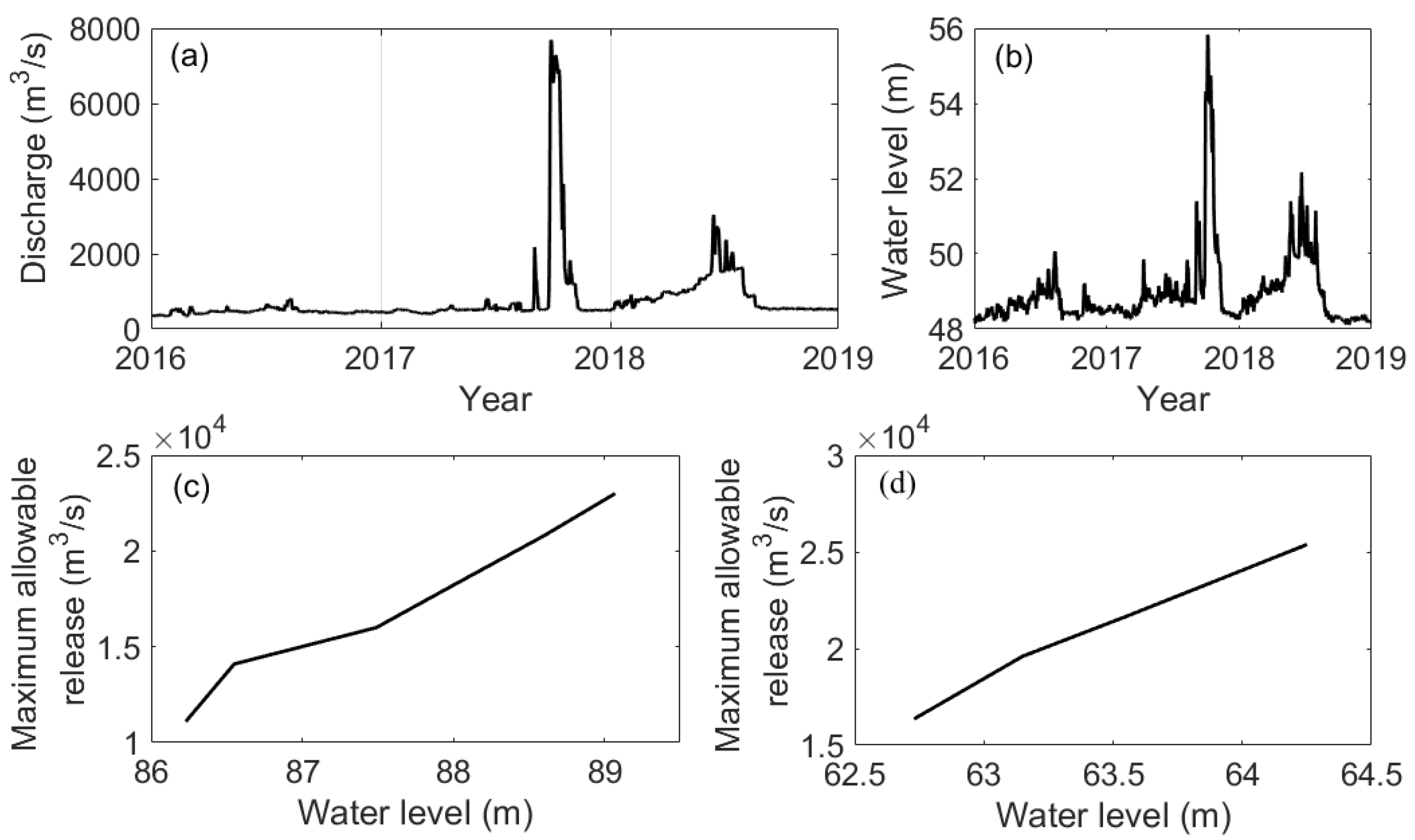
2.1. Study Area

The Han River offers a large amount of biological and hydropower resources and serves as one of the major water sources for the South-to-North Water Diversion in China [42]. Concerning the availability of in-situ hydrometric and satellite altimetry data, a 150 km long reach of Han River in China (Figure 1) is selected to explore the contributions of satellite altimetry-derived datasets on hydrodynamic model calibration. The case area belongs to the middle stream of the Han River between Huangjiagang and Yicheng hydrometric stations. Three main tributaries are located in the study area, and two hydraulic projects, the Wangbuzhou and Cuijiaying reservoirs, are also located with the functions of flood control and hydropower production (Figure 1).

2.2. Data Description

2.2.1. Hydrometric Data

Daily discharge of four hydrometric stations and daily water level of five hydrometric stations from 01/01/2016 to 12/31/2018 are collected from the Bureau of Hydrology, Changjiang Water Resources Commission, affiliated to the Ministry of Water Resources of China (

Table 1. Summary of the hydrometric stations. Q denotes discharge; W denotes water level.

ID	Station Name	Chainage (m)	River Width (m)	Data Type
1	Huangjiagang (HJG)	0	438	Q/W
2	Laohekou (LHK)	20,655	441	W
3	Bei (B)	31,196	101	Q
4	Gucheng (GC)	37,867	182	Q
5	Miaogang (MG)	60,599	280	W
6	Xiangyang (XY)	98,950	534	W
7	Dongcheng (DC)	107,667	351	Q
8	Yicheng (YC)	150,379	650	W
9	Wangbuzhou (WBZ)	28,763	1351	Water control project
10	Cuijiaying (CJY)	113,819	1213

Note: Chainage refers to the distance along the river centerline between points of interest. River width indicates the bank’s full river width from surveyed cross-section river profiles.

). The main-channel geometry of the reach is described by the 94 surveyed cross-section profiles, which are surveyed by the Bureau of Hydrology in 2016. The information on the two hydraulic projects can be found in Table 1 and Figure 2. The operational rules applied for the two projects are dependent on their water levels and water inflows. Specifically, the outflow equals the inflow when the inflow is lower than the maximum allowable release under the normal water level, otherwise, the outflow equals the maximum allowable release under its corresponding water level (Figure 2c,d).

2.2.2. Satellite Altimetry Data

The altimetry-derived WSE are retrieved from Sentinel-3A and CryoSat-2. Sentinel-3A data are collected from the ESA level 2 product “Enhanced measurements”, which are downloaded from the Copernicus Open Access Hub (https://scihub.copernicus.eu/dhus/). The ESA level 2 product contains 20Hz measurements including the waveform, tracker range, satellite altitude, and corrections. The waveforms are retracked with a traditional offset center of gravity retracker [7]. For CryoSat-2, we use the ESA level 1b product from baseline C (https://science-pds.cryosat.esa.int/). The ESA level 1b product contains 20Hz measurements including the waveform, tracker range, satellite altitude, and corrections. The CryoSat-2 waveforms were retracked with a narrow primary peak threshold retracker [43].

The water surface elevations WSE, are constructed via the following equation

$$WSE=h-R-N$$

(1)

where h is the altitude of the satellite, and N is the geoid height, which is the EGM2008 geoid model [44]. R is the range that is the distance from the satellite to the surface, which can be expressed as

$$R=R_{trac}+R_{retrac}+R_{atm}+R_{geo}$$

(2)

where $R_{trac}$ is the distance measured by the onboard tracker, hence the distance to the nominal bin in the waveform and $R_{retrac}$ is the re-tracking correction. $R_{atm}$ is the atmospheric corrections including the wet and dry tropospheric corrections and the ionospheric correction. $R_{geo}$ is the geophysical corrections including solid earth tide, pole tide, and ocean loading tide. All corrections are taken from the altimetry products.

2.3. WSE Data Processing

The altimetry-derived WSE are extracted by a water mask from Global Surface Water Explorer (https://global-surface-water.appspot.com/). Specifically, the maximum extent is used to pre-select as many observations as possible [45].

The identical satellite ground tracks with a repeat cycle of 27 days allow to derive the WSE time series at two virtual stations (VSs) from Sentinel-3A over the study reach (Figure 1). Firstly, the outliers are discarded by comparing the altimetry-derived WSE with ASTER GDEM v.3 (Advanced Spaceborne Thermal Emission and Reflection Radiometer Global Digital Elevation Model) [46] with an absolute bias threshold of 20 m. The DEM datasets have been reprojected to the EGM2008 geoid at the platform of VDatum software [47]. Secondly, a filtering process is performed for each track to discard outliers based on the work by Jiang et al. [40] and finally, the median value of all WSE observations for a given track is used to derive WSE time series. The data processing for CryoSat-2 altimetry is slightly different from that of Sentinel-3A due to its drifting ground track pattern. A series of virtual stations were selected and all observations were relocated to the nearest virtual stations based on their local slopes [43]. The virtual stations are determined based on the coverages of CryoSat-2 observations along the river reach and placed on the model river line (i.e., the centerline of the river from the extracted water mask). The procedure of relocating CryoSat-2 observations onto virtual stations has been proved to be an efficient way of constructing WSE time series at VSs and strengthening the hydrologic and hydrodynamic applications of CryoSat-2 [43]. Balancing the maximization of the VS numbers and the minimization of error from projecting observations to virtual stations, 16 VSs have been figured out in the study reach (

Table 2. Characteristics of each virtual station from the Sentinel-3A and CryoSat-2 missions.

ID	Lon (degree)	Lat (degree)	Chainage (m)	Width (m)	Number
VS Platform: CryoSat-2
1	111.539	32.485	3681	1060	3
2	111.605	32.459	114,59	1494	3
3	111.666	32.401	193,53	1351	5
4	111.688	32.286	32,570	575	3
5	111.704	32.191	42,175	604	3
6	111.768	32.155	51,246	348	3
7	111.905	32.069	69,674	563	5
8	111.981	32.086	80,502	862	4
9	112.053	32.042	87,091	749	2
10	112.18	32.037	92,876	1290	3
11	112.194	31.987	104,022	1068	3
12	112.16	31.955	113,369	1206	1
13	112.205	31.907	121,534	776	3
14	112.208	31.857	129,284	434	2
15	112.192	31.772	140,443	403	2
16	112.241	31.750	146,961	571	4
VS Platform: Sentinel-3A
1	111.579	32.467	7654	775	36
2	112.109	32.025	94,622	1253	38

Note: VS indicates the virtual stations. Width indicates the bank full river width from surveyed cross-section river profiles. The number indicates the number of processed median observations at each virtual station applied for hydrodynamic modeling.

). An outlier filtering algorithm is performed to obtain the median values of each track: a measurement is discarded if |h-u|>3δ (h is the point observation, u is the mean value and δ is the standard deviation) [40]. All the median observations are relocated to the nearest virtual stations through local slope correction. It should be noted that there are often systematic biases between satellite altimetry-derived observations and in-situ data due to the unknown local vertical datums and other factors. If their mean values of every series are removed, both in-situ data and satellite altimetry-derived datasets are transformed to WSE anomalies.

2.4. Hydrodynamic Model in the Study Area

A one-dimension (1D) hydrodynamic model is used to simulate flow regimes and water levels of the study reach. The model was running at the DHI MIKE 11 software [48]. The software solves the Saint–Venant equations with an implicit 6-point finite-difference scheme. The model is directly forced by the observed daily discharge data from the main upstream and three tributaries, while the daily water level of Yicheng hydrometric station is served as the downstream boundary condition (shown in Figure 1). The study reach is sketched by 94 cross-section profiles, and the profiles are derived from the detailed bathymetric map with an interval of around 50 m and thus can capture the variations of riverbed geometry. The operational rules of Wangbuzhou and Cuijiaying reservoirs are also simulated in the model as it is described in Section 2.2.

2.5. Hydrodynamic Model Calibration

The hydrodynamic model calibration focuses on the estimation of the channel roughness, i.e., the Strickler coefficient Ks (the reciprocal of the Manning coefficient, see in Manning’s Equation (3)).

$$Q=A{r}^{\frac{2}{3}}{S}^{\frac{1}{2}}{K}_s$$

(3)

With given bathymetry data, the cross-section area (A), the hydraulic radius (r), the slope of the hydraulic gradient line (S) at the discharge (Q) can be described as a function of water depth relating to WSE. Only Ks is a parameter that varies along the river and is often calibrated through maximizing the degree of goodness of fit between observed and simulated WSE. To figure out the effect of heterogeneity of roughness distribution on model performance, two roughness cases are assumed in the calibration process. One is that only a single Ks coefficient is assigned to the whole reach (uniform Ks). The other one is that the river reach is partitioned into sub-reaches according to the hydro-morphological characteristics of the river and the distribution of hydrometric stations (variable Ks). The variable Ks with sub-reaches has also been proved to be a feasible approach to improve the hydrodynamic model performance [34]. Specifically, four sub-reaches are used in our case study for the variable Ks. The first 29 km long reach is very gentle (0.035 m/km) and the following 44 km long reach is narrow and steep with a complex river morphology. In the following 38 km long reach, the river channel is steeper with a gradient of 0.125 m/km. The last reach is a little wider and deeper.

To investigate the efficiency and reliability of the various satellite altimetry-derived datasets, three configurations are constructed for the hydrodynamic model calibration. The first one is from the in-situ data (called Configuration A), the second one is from the altimetry-derived data from Sentinel-3A and CryoSat-2 (called Configuration B) and the last one is from the combination of in-situ and satellite altimetry-derived data (called Configuration C). Combining the three configurations and two roughness cases, there are fourteen scenarios for calibrating the hydrodynamic model as shown in

Table 3. Summary of hydrodynamic model calibration.

Scenarios Design		Using In-Situ	Using Sentinel-3A	Using CryoSat-2
Configuration A: using in-situ data (two schemes)
AU1	AV1	Y	-	-
Configuration B: using satellite altimetry data (six schemes)
BU1	BV1	-	Y	-
BU2	BV2	-	-	Y
BU3	BV3	-	Y	Y
Configuration C: using both in-situ and satellite altimetry data (six schemes)
CU1	CV1	Y	Y	-
CU2	CV2	Y	-	Y
CU3	CV3	Y	Y	Y

Note: Y indicates objective function. U/V indicate the uniform and variable roughness cases, respectively. 1, 2, 3 indicate the number of data sources in the corresponding configuration A, B, and C.

.

The 1D hydrodynamic model is calibrated by the fourteen scenarios from 01/01/2016 to 12/31/2017 through minimizing the Root Mean Square Error (RMSE) between simulated and observed WSE. The model is also validated by the data from 01/01/2018 to 12/31/2018. The manual trial-and-error method is adopted for testing the variable Ks case and the scenario-based method is used (running models with a range of values of Ks at an interval of 0.5/0.1 m^1/3s⁻¹) for the uniform Ks case [33,49].

$$RMSE=\sqrt{\frac{1}{n}{\displaystyle \sum _{i=1}^n{({\widehat{p}}_i-o_i)}^2}}$$

(4)

where O_i and ${\widehat{p}}_i$ are the observed and simulated WSE at the ith point, respectively. n is the total number of WSE observations.

3. Results

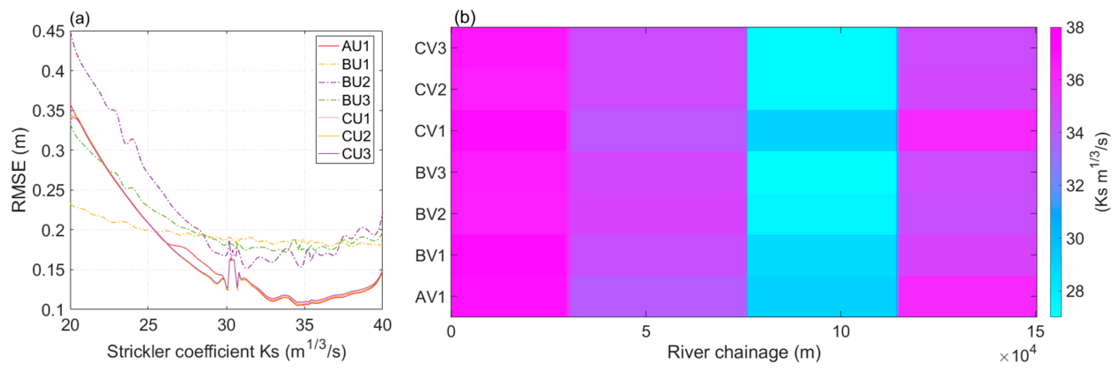
3.1. Calibrated Strickler Coefficient Ks

The calibrated uniform Ks plays a vital role in hydrodynamic simulation, and the optimal Ks value can be easily determined from the clear patterns shown in Figure 3a (e.g., 34.6 m^1/3/s as the optimal value for the scheme AU1). The model performance is sensitive to uniform Ks value (RMSE ranging from 0.105–0.450 m) and the optimal RMSE values are assigned near the high bound of the parameter range. The calibrated Ks values of four sub-reaches reflect the characteristics of each sub-reach (Figure 3b). The Ks values of the second and the final sub-reaches range from 27–33 m^1/3/s. The Ks is relatively high at the first upstream 29-km reach (approximately 37 m^1/3/s) due to the flat and straight river channel. On the contrary, the Ks value has decreased significantly in the third reach due to the increasing water depth and highly vegetated channel. Roughness is closely related to flow resistance, which is positively influenced by river depth and vegetable conditions. More specifically, flow resistance increases with a highly vegetated channel and river depth, and leads to higher roughness (smaller Ks) [49,50]. It is interesting to find that the RMSE values jump near the Strickler coefficient close to 30 in Figure 3a. As there are discharge bursts in 2017 that can challenge the calibration of parameters (Figure 2a), the RMSE value is sensitive to the bias of peak simulation. The peaks of discharge should be processed separately and the model parameters (Ks) should be chosen in a special way. There is not enough available data (in-situ records and satellite observations) to separately calibrate the parameters. In addition, all the jumping curves are from the uniform Ks scenarios, which proves that the uniform parameter can bring more uncertainties of discharge simulation and cut down the contribution of the satellite altimetry-derived WSE to hydrodynamic model calibration at the whole river reach.

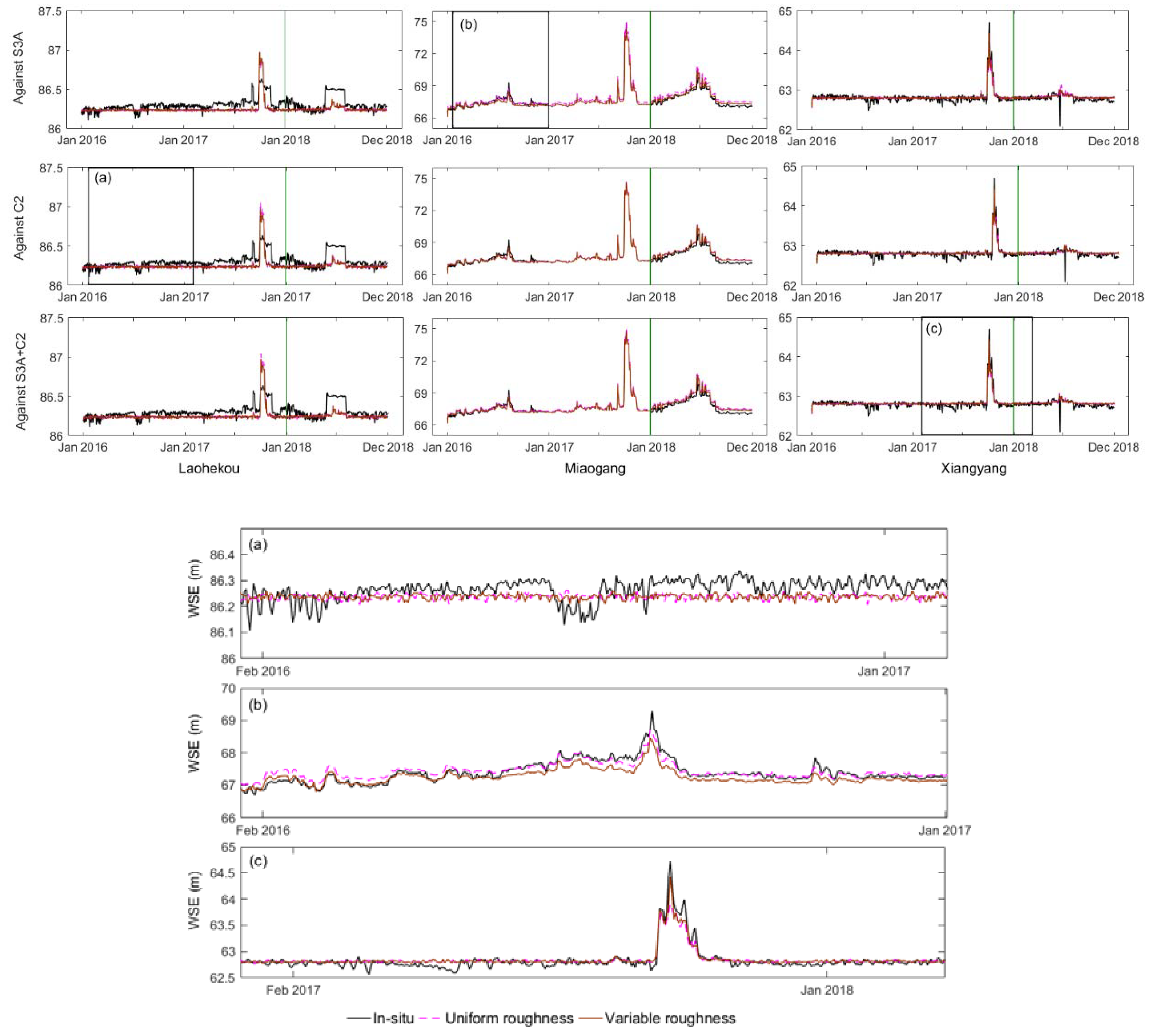
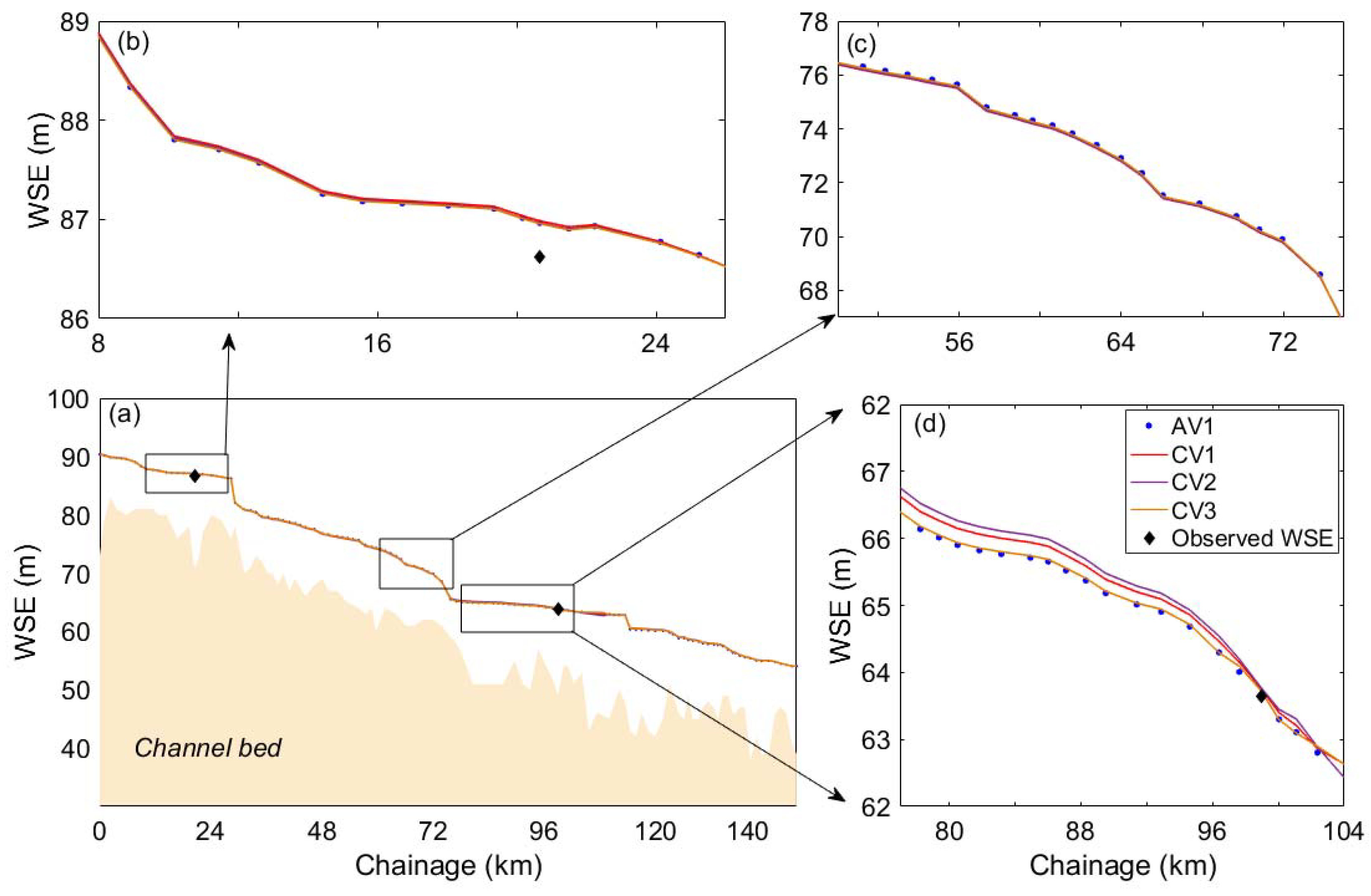
3.2. Hydrodynamic Model Performances with Different Configurations

3.2.1. Model Calibration with the in-situ Observations

Regarding configuration A, hydrodynamic models are calibrated by the in-situ observations using the uniform and variable Ks (i.e., the schemes AU1 and AV1). The results during the calibration and validation periods reveal that the model can reproduce WSE well, where the RMSE ranging from 0.100–0.216 m (

Table 4. Summary of statistical metrics of average model performance in terms of RMSE at all stations of the schemes.

Schemes	RMSE (m)		Schemes	RMSE (m)
	Calibration	Validation		Calibration	Validation
AU1	0.105	0.204	AV1	0.100	0.216
BU1	0.179	0.146	BV1	0.177	0.148
BU2	0.154	0.313	BV2	0.153	0.316
BU3	0.172	0.227	BV3	0.168	0.234
CU1	0.108	0.202	CV1	0.104	0.210
CU2	0.106	0.206	CV2	0.102	0.204
CU3	0.109	0.205	CV3	0.105	0.205

Note: Details of calibration and validation conditions can be found in Table 3.

). However, there are few obvious differences in the accuracies of WSE simulation from the two roughness cases. The averaged performances from the variable Ks are slightly better than those from the uniform Ks during the calibration periods while the results are not as good as those from the uniform Ks during the validation periods. Nevertheless, the improved results from the variable Ks can be found with lower RMSE values at the specific station (Figure 4 and Figure 5). For example, the RMSE from the variable Ks is 0.074 m at Xiangyang station, decreased by 11.5% compared to that from the uniform Ks (Figure 5). Overall, the improvements with the variable Ks highlight the potential superiority of the variable Ks in hydrodynamic model calibration.

3.2.2. Model Calibration with the Satellite Altimetry-derived Observations

Concerning configuration B, the model is calibrated by the satellite altimetry-derived WSE. There are six model scenarios, i.e., calibration by Sentinel-3A, CryoSat-2, and the combinations of these two datasets taking the uniform and variable Ks cases (see the details in Table 3). The calibrated models show the comparable performance in comparison to those by using in-situ data in terms of RMSE values during both calibration and validation periods where the RMSE ranges 0.153–0.179 m in Table 4. Thus, the altimetry-derived datasets from Sentinel-3A and CryoSat-2 can be applied in the hydrodynamic model calibration. However, the contributions of WSE from different altimetry to hydrodynamic model calibration are different. The schemes BU(V)2 (against CryoSat-2) show the lowest values of RMSE while the schemes BU(V)1 (against Sentinel-3A) perform worst during the calibration periods. Interestingly, the model calibrated by the schemes BU(V)2 shows the best performance in the calibration period while it performs worst in the validation period probably due to their different sample size during the calibration and validation periods. The simulated WSE at virtual stations from the variable Ks consistently shows a better performance than those from the uniform Ks. The distributions of difference between model simulations and satellite altimetry-derived WSE have also been shown in Figure 6 and Figure 7, which further proves the advantages of the variable Ks.

To show the performances of hydrodynamic model calibrated by altimetry-derived datasets at three in-situ stations, their statistical metrics (RMSE) are shown in Figure 5 and their hydrographs are depicted in Figure 8. The models calibrated by satellite altimetry-derived datasets can also provide reliable WSE estimations at these in-situ stations. Moreover, the statistical metrics are different for every station due to their flow regimes and channel geometry. For example, WSE estimations at Miaogang station are not as good as those at other two in-situ stations with higher RMSE values (Figure 5). The model performance can also be dependent on the schemes with different satellite altimetry-derived datasets or roughness cases. The schemes BU(V)2 (against CryoSat-2) show better skills than the schemes BU(V)1 (against Sentinel-3A) or BU(V)3 (against all satellite altimetry-derived datasets) in simulating WSE at in-situ stations (Figure 5). For example, the RMSE values from the scheme BU2 at Miaogang station are 0.158/0.316 m for the calibration/validation periods, while the RMSE values from the schemes BU1 and BU3 are 0.162/0.420 and 0.162/0.306 m, respectively.

3.2.3. Model Calibration with Both In-Situ and Satellite Altimetry-Derived Observations

In the case of configuration C, the hydrodynamic model was calibrated by all available observations at in-situ and virtual stations. The contributions of additional satellite altimetry-derived WSE to hydrodynamic model calibration are relatively small at the evaluated in-situ and virtual stations (Table 4). This can be attributed to the fact that the temporal resolution of the available in-situ observations (daily frequency) is higher than that of satellite altimetry-derived datasets (e.g., 27-day frequency for S3A observations). Despite the little contribution, the advantages of additional satellite altimetry-derived datasets to the hydrodynamic model can still be found through the reproduction of the flood event (i.e., the flow processes with the maximum discharge at the upper boundary) (Figure 9). The WSE obtained from the model by calibration using all available observations is different from that obtained by calibration using only in-situ observations in the region where the satellite altimetry-derived observations can be found (shown in Figure 9d). With more spatially-distributed WSE observations, the hydrodynamic model provides more reliable WSE estimations on the whole river reach. The integration of altimetry-derived datasets and in-situ observations has led to the best performance for the hydrodynamic model calibration. Therefore, the satellite altimetry-derived datasets can be taken as a significant complementary to in-situ gauging networks, especially for improving the reliable simulation of WSE at the whole river reach scale.

4. Discussion

4.1. Effects of Satellite Altimetry-Derived WSE on Hydrodynamic Model Calibration

Two pivotal factors are influencing the performance of the hydrodynamic model calibrated by satellite altimetry-derived WSE. One is the accuracy of satellite data itself and the other one is the spatio-temporal resolution of satellite altimetry missions. The two VSs of Sentinel-3A (i.e., VS1 and VS2) are close to the Huangjiagang and Xiangyang hydrometric stations (eight km from VS1 to Huangjiagang, four km from VS2 to Xiangyang). The slopes between the two VSs and their corresponding hydrometric stations are too flat to impact the WSE. The WSE at the two VSs can replace the data observed at the Huangjiagang and Xiangyang stations. The RMSE values are 0.28 m and 0.16 m for the VS1 and VS2, respectively. In the same way, the accuracies of CryoSat-2 at VS3 and VS7 are also evaluated by the observation data from Lianghekou (one km from VS3) and Xiangyang (eight km from VS7). The RMSE values are 0.14 m and 0.71 m for the VS3 and VS7, respectively. According to the previous studies [7,51], the RMSE values for satellite altimetry below 0.3 m are taken as good, and below 0.6 m are moderate. Sentinel-3A and CryoSat-2 data are not only found to be good and moderate in the literature [7,34,43] but also have been proved to be good and moderate in our case study river, a medium river (around 400 m) with braided and single-threaded reaches. By discarding outliers based on DEM approaches, a good or moderate accuracy of altimetry observations can be obtained in the case study, indicating that the land relief issue can be well addressed by discarding invalid measurements (e.g., a careful analysis of satellite waveforms identification). Our findings suggest that a good or moderate accuracy of altimetry observations can provide satisfactory results for hydrodynamic model calibration.

The spatio-temporal resolution of satellite altimetry missions directly influences the performance of hydrodynamic model calibration. Our findings further revealed that CryoSat-2 geodetic altimetry with high spatial resolution shows better performance in hydrodynamic model calibration than Sentinel-3A altimetry with a low spatial resolution (Table 4 and Figure 3, Figure 4 and Figure 5). It should be noted that CryoSat-2 geodetic altimetry has a full cycle of 369 days while Sentinel-3A has a 27-day cycle at the specified virtual stations. The values of the new Sentinel-3A altimetry to hydrodynamic model calibration are highlighted due to its high data-quality with a new on-board tracking mode and easier work in deriving WSE time series at virtual stations. But it is challenging to process the spatially-distributed CryoSat-2 observations and use them for hydrodynamic model calibration [34,39]. In our case study, the CryoSat-2 data are relocated onto a series of virtual stations and then transformed into anomalies for hydrodynamic model calibration [43]. The systematic bias still remains when processing such few CryoSat-2 observations into anomalies, and can be propagated into WSE simulation of the model and reduces its accuracy. This could be attributed to the fact that the results are not the best among the schemes of configuration B when pooling the Sentinel-3A and CryoSat-2 datasets for model calibration (shown in Table 4 and Figure 3, Figure 4 and Figure 5). Further works can focus on producing blending products with more densified data from different satellite altimetry missions through the statistical and hydraulic blending approaches and use them for hydrodynamic modeling [52,53].

4.2. Comparison of Model Performance from Uniform and Variable Roughness Parameters

The effects of the two parameterizations on hydrodynamic model calibration have been reported in the literature [30,34], and are further explored on the use of various altimetry-derived datasets in our case study. The uniform Ks is widely used in hydrodynamic model calibration for its simplicity and promising efficiency at the evaluated stations. However, this common approach fails to characterize the variations of the riverbed and is probably unable to reproduce accurate WSE at other locations of the river under high heterogeneity [4,54]. The hydrodynamic model with uniform Ks calibrated by Sentinel-3A derived-WSE shows poor skills with high RMSE values at in-situ stations (Figure 5). Moreover, the uniform Ks can also be attributed to the equifinality issue, i.e., a model with different roughness sets performs equally well at the evaluated gauging stations (shown in Figure 3a). To find a more efficient approach for more accurate WSE estimation along the river under the heterogeneity of the channel, the variable Ks is recommended for hydrodynamic model calibration as it takes the spatial variability of flow resistance into account [34]. The model with the variable Ks can simulate WSE more accurately with lower RMSE values compared to that with the uniform Ks.

Two pivotal factors are influencing the hydrodynamic model calibration with the variable Ks. One is the availability of data for model calibration and the other is the density of resolved variable roughness parameters. With satellite altimetry-derived data available, the variable Ks could be an efficient approach to facilitate hydrodynamic modeling. The model performance is also closely dependent on the satellite altimetry datasets with different spatio-temporal resolution. The CryoSat-2 geodetic mission with dense observations is more helpful than those with a low spatial resolution (Sentinel-3A) in hydrodynamic model calibration (Table 4 and Figure 3, Figure 4 and Figure 5). The contributions of the densified roughness parameters on model calibration have been highlighted in the literature [4,34], while the improvements of the densified roughness parameters come at the expense of uncertainties and computation time. The more parameters commonly required more data for calibration [4]. Schneider et al. [34] used the 10-km variable roughness parameters to facilitate hydrodynamic modeling and found that the performances of the model were not refined well with large uncertainties. This issue is further revealed in our case study that the accuracies of WSE from the variable Ks are slightly better than those from the uniform Ks during the calibration periods with reducing RMSE values by 2–14%, while the results are not as good as those from the uniform Ks during the validation periods. However, the advantages of the variable Ks are not only to improve the accuracy of simulated WSE at the evaluated gauging stations but also to improve the hydrodynamic simulation on the entire river reach via a physically-based strategy. With more satellite altimetry-derived WSE available, the variable Ks could be estimated well and therefore increases the performance of the hydrodynamic model [55]. As the calibrated Ks values are reasonable compared to previous works [34,56], the variable Ks is recommended for hydrodynamic model calibration.

5. Conclusions

The contributions of current satellite altimetry missions (i.e., short-repeat and geodetic altimetry) on hydrodynamic model calibration are reviewed. The contribution of the new Sentinel-3A altimetry is also assessed. Hydrodynamic model (DHI MIKE 11) calibrations with available bathymetry data are carried out by combining seven calibration datasets (i.e., in-situ, satellite altimetry, and both of them) and two roughness cases (i.e., spatially variable roughness and uniform roughness). In the case study river reach with a river width of around 400 m, both Sentinel-3A and CryoSat-2 can deliver useful observations with the averaged RMSE values of 0.22 and 0.49 m, respectively. Our findings suggest that a good or moderate accuracy of altimetry observations (RMSE below 0.6 m) can contribute to the hydrodynamic model calibration. Specifically, calibration against altimetry-derived WSE achieves promising results in terms of RMSE as 0.100­–0.216 m during the calibration periods, which are in line with previous studies [30,34]. Moreover, model performance varies with different altimetry-derived datasets due to their different characteristics such as spatio-temporal sampling patterns.

Although the satellite altimetry has a low temporal resolution, both Sentinel-3A and CryoSat-2 can provide a comparable result as those from the daily in-situ observations. CryoSat-2 with a higher spatial resolution (7.5 km at the Equator) brings better performances than short-repeat Sentinel-3A altimetry with a low resolution (104 km at the Equator) in the hydrodynamic model calibration according to their RMSE values of 0.16 and 0.18 m, respectively. Moreover, the variable Ks improves the performance of hydrodynamic simulation compared to the uniform Ks reducing the RMSE values by 2–14%, and is recommended in hydrodynamic model calibration for its physically-based strategy. Our study not only enriches the existing knowledge on integrating satellite altimetry-derived datasets into hydrodynamic model calibration but also supports the future hydrology-related satellite altimetry design.

References

1. Mann, M.E.; Rahmstorf, S.; Kornhuber, K.; Steinman, B.A.; Miller, S.K.; Coumou, D. Influence of Anthropogenic climate change on planetary wave resource and extreme weather events. Sci. Rep. 2017, 7, 45242. [Google Scholar] [CrossRef] [Green Version]
2. Yin, J.; Gentine, P.; Zhou, S.; Sullivan, S.C.; Wang, R.; Zhang, Y.; Guo, S. Large increase in global storm runoff extremes driven by climate and anthropogenic changes. Nat. Commun. 2018, 9, 4389. [Google Scholar] [CrossRef] [Green Version]
3. Blari, P.; Buytaert, W. Socio-hydrological modelling: A review asking “why, what and how?”. Hydrol. Earth Syst. Sci. 2016, 20, 443–478. [Google Scholar] [CrossRef] [Green Version]
4. Jiang, L.; Bandini, F.; Smith, O.; Jensen, I.K.; Bauer-Gottwein, P. The value of distributed high-resolution UAV-Borne observations of water surface elevation for river management and hydrodynamic modeling. Remote Sens. 2020, 12, 1171. [Google Scholar] [CrossRef] [Green Version]
5. Normandin, C.; Frappart, F.; Diepkilé, A.T.; Marieu, V.; Mougin, E.; Blarel, F.; Lubac, B.; Braquet, N.; Ba, A. Evaluation of the performance of radar altimetry missions from ERS-2 to Sentinel-3A over the Inner Niger Delta. Remote Sens. 2018, 10, 833. [Google Scholar] [CrossRef] [Green Version]
6. Hossain, F.; Maswood, M.; Siddique-E-Akbor, A.H.; Yigzaw, W.; Mazumdar, L.C.; Ahmed, T.; Hossain, M.; Shah-Newaz, S.M.; Limaye, A.; Lee, H.; et al. A promising radar altimetry satellite system for operational flood forecasting in flood-prone Bangladesh. IEEE Geosci. Remote Sens. Mag. 2014, 2, 27–36. [Google Scholar] [CrossRef]
7. Kittel, C.M.M.; Jiang, L.; To, C.; Bauer-Gottwein, P. Sentinel-3 radar altimetry for river monitoring—A catchment-scale evaluation of satellite water surface elevation from Sentinel-3A and Sentinel-3B. Hydrol. Earth Syst. Sci. Discuss. 2020, 165. [Google Scholar] [CrossRef]
8. Biancamaria, S.; Hossain, F.; Lettenmaier, D.P. Forecasting transboundary river water elevations from space. Geophys. Res. Lett. 2011, 38, 1–5. [Google Scholar] [CrossRef] [Green Version]
9. Da Silva, J.S.; Calmant, S.; Seyler, F.; Moreira, D.M.; Oliveira, D.; Monteiro, A. Radar altimetry aids managing gauge networks. Water Resour. Manag. 2014, 28, 587–603. [Google Scholar] [CrossRef]
10. Tauro, F.; Selker, J.; van de Giesen, N.; Abrate, T.; Uijlenhoet, R.; Porfiri, M.; Manfreda, S.; Caylor, K.; Moramarco, T.; Benveniste, J.; et al. Measurements and observations in the XXI century (MOXXI): Innovation and multi-disciplinarily to sense the hydrological cycle. Hydrol. Earth Syst. Sci. 2018, 63, 169–196. [Google Scholar] [CrossRef] [Green Version]
11. Siddique-E-Akbor, A.H.M.; Hossain, F.; Lee, H.; Shum, C.K. Inter-comparison study of water level estimates derived from hydrodynamic-hydrologic model and satellite altimetry for a complex deltaic environment. Remote Sens. Environ. 2011, 115, 1522–1531. [Google Scholar] [CrossRef]
12. García-Pintado, J.; Neal, J.C.; Mason, D.C.; Dance, S.L.; Bates, P.D. Scheduling satellite-based SAR acquisition for sequential assimilation of water level observations into flood modelling. J. Hydrol. 2013, 495, 252–266. [Google Scholar] [CrossRef] [Green Version]
13. Tarpanelli, A.; Brocca, L.; Melone, F.; Moramarco, T. Hydraulic modelling calibration in small rivers by using coarse resolution synthetic aperture radar imagery. Hydrol. Process. 2013, 27, 1321–1330. [Google Scholar] [CrossRef]
14. de Moraes Frasson, R.P.; Wei, R.; Durand, M.; Minear, J.T.; Domeneghetti, A.; Schumann, G.; Williams, B.A.; Rodriguez, E.; Picamilh, C.; Lion, C.; et al. Automated river reach definition strategies: Applications for the surface water and ocean topography mission. Water Resour. Res. 2017, 53, 8164–8186. [Google Scholar] [CrossRef]
15. Hostache, R.; Matgen, P.; Schumann, G.; Puech, C.; Hoffmann, L.; Pfister, L. Water level estimation and reduction of hydraulic model calibration uncertainties using satellite SAR images of floods. IEEE Trans. Geosci. Remote Sens. 2009, 47, 431–441. [Google Scholar] [CrossRef]
16. Birkinshaw, S.J.; O’Donnell, G.M.; Moore, P.; Kilsby, C.G.; Fowler, H.J.; Berry, P.A.M. Using satellite altimetry data to augment flow estimation techniques on the Mekong River. Hydrol. Process. 2010, 24, 3811–3825. [Google Scholar] [CrossRef]
17. Michailovsky, C.I.; Milzow, C.; Bauer-Gottwein, P. Assimilation of radar altimetry to a routing model of the Brahmaputra River. Water Resour. Res. 2013, 49, 4807–4816. [Google Scholar] [CrossRef]
18. Schneider, R.; Godiksen, P.N.; Villadsen, H.; Madsen, H.; Bauer-Gottwein, P. Application of CryoSat-2 altimetry data for river analysis and modelling. Hydrol. Earth Syst. Sci. 2017, 21, 751–764. [Google Scholar] [CrossRef] [Green Version]
19. Biancamaria, S.; Frappart, F.; Leleu, A.-S.; Marieu, V.; Blumstein, D.; Desjonquères, J.-D.; Boy, F.; Sottolichio, A.; Valle-Levinson, A. Satellite radar altimetry water elevations performance over a 200 m wide river: Evaluation over the Garonne River. Adv. Space Res. 2017, 59, 128–146. [Google Scholar] [CrossRef] [Green Version]
20. Birkinshaw, S.J.; Moore, P.; Kilsby, C.G.; O’Donnell, G.M.; Hardy, A.J.; Berry, P.A.M. Daily discharge estimation at ungauged river sites using remote sensing. Hydrol. Process. 2014, 28, 1043–1054. [Google Scholar] [CrossRef]
21. Sulistioadi, Y.B.; Tseng, K.H.; Shum, C.K.; Hidayat, H.; Sumaryono, M.; Suhardiman, A.; Setiawan, F.; Sunarso, S. Satellite radar altimetry for monitoring small rivers and lakes in Indonesia. Hydrol. Earth Syst. Sci. 2015, 19, 341–359. [Google Scholar] [CrossRef] [Green Version]
22. Ablain, M.; Meyssignac, B.; Zawadzki, L.; Jugier, R.; Ribes, A.; Spada, G.; Benveniste, J.; Cazenave, A.; Picot, N. Uncertainty in satellite estimates of global mean sea-level changes, trend and acceleration. Earth Syst. Sci. Data 2019, 11, 1189–1202. [Google Scholar] [CrossRef] [Green Version]
23. Goumehei, E.; Tolpekin, V.; Stein, A.; Yan, W. Surface water body detection in polarimetric SAR data using contextual complex Wishart classification. Water Resour. Res. 2019, 55, 7047–7059. [Google Scholar] [CrossRef] [Green Version]
24. Weekley, D.; Li, X. Tracking multidecadal lake water dynamics with Landsat imagery and topography/bathymetry. Water Resour. Res. 2019, 55, 8350–8367. [Google Scholar] [CrossRef]
25. Haque, M.M.; Seidou, O.; Mohammadian, A.; Djibo, A.G. Development of a time-varying MODIS/2D hydrodynamic model relationship between water levels and flooded areas in the Inner Niger Delta, Mali, West Africa. J. Hydrol. Reg. Stud. 2020, 30, 100703. [Google Scholar] [CrossRef]
26. Mtamba, J.; Van der Velde, R.; Ndomba, P.; Zoltán, V.; Mtalo, F. Use of Radarsat-2 and Landsat TM images for spatial parameterization of Manning’s roughness coefficient in hydraulic modeling. Remote Sens. 2015, 7, 836–864. [Google Scholar] [CrossRef] [Green Version]
27. Paiva, R.C.D.; Collischonn, W.; Buarque, D.C. Validation of a full hydrodynamic model for large-scale hydrologic modelling in the Amazon. Hydrol. Process. 2011, 27, 333–346. [Google Scholar] [CrossRef]
28. Chen, H.; Liang, Z.; Liu, Y.; Liang, Q.; Xie, S. Integrated remote sensing imagery and two-dimensional hydraulic modeling approach for impact evaluation of flood on crop yields. J. Hydrol. 2017, 553, 262–275. [Google Scholar] [CrossRef] [Green Version]
29. Andreadis, K.M. Data assimilation and river hydrodynamic modeling over large scales. In Global Flood Hazard: Applications in Modeling, Mapping, and Forecasting; American Geophysical Union: Washington, DC, USA, 2018. [Google Scholar] [CrossRef]
30. Domeneghetti, A.; Tarpanelli, A.; Brocca, L.; Barbetta, S.; Moramarco, T.; Castellarin, A.; Brath, A. The use of remote sensing-derived water surface data for hydraulic model calibration. Remote Sens. Environ. 2014, 149, 130–141. [Google Scholar] [CrossRef]
31. Dettmering, D.; Ellenbeck, L.; Scherer, D.; Schwatke, C.; Niemann, C. Potential and limitations of satellite altimetry constellations for monitoring surface water storage changes—A case study in the Mississippi Basin. Remote Sens. 2020, 12, 3320. [Google Scholar] [CrossRef]
32. Biancamaria, S.; Lettenmaier, D.P.; Pavelsky, T.M. The SWOT mission and its capabilities for land hydrology. Surv. Geophys. 2016, 37, 307–337. [Google Scholar] [CrossRef] [Green Version]
33. Garambois, P.A.; Calmant, S.; Roux, H.; Paris, A.; Monnier, J.; Finaud-Guyot, P.; Montazem, A.S.; da Silva, J.S. Hydraulic visibility: Using satellite altimetry to parameterize a hydraulic model of an ungauged reach of a braided river. Hydrol. Process. 2017, 31, 756–767. [Google Scholar] [CrossRef] [Green Version]
34. Schneider, R.; Tarpanelli, A.; Nielsen, K.; Madsen, H.; Bauer-Gottwein, P. Evaluation of multi-mode CryoSat-2 altimetry data over the Po River against in situ data and a hydrodynamic model. Adv. Water Resour. 2018, 112, 17–26. [Google Scholar] [CrossRef] [Green Version]
35. Liu, G.; Schwartz, F.W.; Tseng, K.-H.; Shum, C.K. Discharge and water-depth estimates for ungauged rivers: Combining hydrologic, hydraulic and inverse modeling with stage and water-area measurements from satellites. Water Resour. Res. 2015, 51, 6017–6035. [Google Scholar] [CrossRef]
36. Getirana, A.C.V.; Peters-Lidard, C. Estimating water discharge from large radar altimetry datasets. Hydrol. Earth Syst. Sci. 2013, 17, 923–933. [Google Scholar] [CrossRef] [Green Version]
37. Jiang, L.; Madsen, H.; Bauer-Gottwein, P. Simultaneous calibration of multiple hydrodynamic model parameters using satellite altimetry observations of water surface elevation in the Songhua River. Remote Sens. Environ. 2019, 225, 229–247. [Google Scholar] [CrossRef]
38. Donlon, C.; Berruti, B.; Buongiorno, A.; Ferreira, M.-H.; Féménias, P.; Frerick, J.; Goryl, P.; Klein, U.; Laur, H.; Mavrocordatos, C.; et al. The global monitoring for environment and security (GMES) Sentinel-3 mission. Remote Sens. Environ. 2012, 120, 37–57. [Google Scholar] [CrossRef]
39. Jiang, L.; Schneider, R.; Andersen, O.B.; Bauer-Gottwein, P. CryoSat-2 altimetry applications over rivers and lakes. Water 2017, 9, 211. [Google Scholar] [CrossRef]
40. Jiang, L.; Nielsen, K.; Andersen, O.B.; Bauer-Gottwein, P. CryoSat-2 radar altimetry for monitoring freshwater resources of China. Remote Sens. Environ. 2017, 200, 125–139. [Google Scholar] [CrossRef] [Green Version]
41. Wingham, D.J.; Francis, C.R.; Baker, S.; Bouzinac, C.; Brockley, D.; Cullen, R.; de Chateau-Thierry, P.; Laxon, S.W.; Mallow, U.; Mavrocordatos, C.; et al. CryoSat: A mission to determine the fluctuations in Earth’s land and marine ice fields. Adv. Space Res. 2006, 37, 841–871. [Google Scholar] [CrossRef]
42. Liu, D.; Guo, S.; Shao, Q.; Liu, P.; Xiong, L.; Wang, L.; Hong, X.; Xu, Y.; Wang, Z. Assessing the effects of adaptation measures on optimal water resources allocation under varied water availability conditions. J. Hydrol. 2018, 556, 759–774. [Google Scholar] [CrossRef]
43. Villadsen, H.; Andersen, O.B.; Stenseng, L.; Nielsen, K.; Knudsen, P. CryoSat-2 altimetry for river level monitoring-Evaluation in the Ganges-Brahmaputra River basin. Remote Sens. Environ. 2015, 168, 80–89. [Google Scholar] [CrossRef]
44. Pavlis, N.K.; Holmes, S.A.; Kenyon, S.C.; Factor, J.K. The development and evaluation of the Earth Gravitational Model 2008 (EGM2008). J. Geophys. Res. Solid Earth 2012, 117. [Google Scholar] [CrossRef] [Green Version]
45. Pekel, J.-F.; Cottam, A.; Gorelick, N.; Belward, A.S. High-resolution mapping of global surface water and its long-term changes. Nature 2016, 540, 418–422. [Google Scholar] [CrossRef] [PubMed]
46. ASTER GDEM Validation Team. ASTER Global DEM Validation. Summary Report; 2009; pp. 1–28. Available online: https://ssl.jspacesystems.or.jp/ersdac/GDEM/E/image/ASTERGDEM_ValidationSummaryReport_Ver1.pdf (accessed on 11 December 2020).
47. Myers, E.; Hess, K.; Yang, Z.; Xu, J.; Wong, A.; Doyle, D.; Woolard, J.; White, S.; Le, B.; Gill, S.; et al. VDatum and strategies for national coverage. In Proceedings of the Ocean Conference Record (IEEE), Vancouver, BC, Canada, 29 September–4 October 2007. [Google Scholar] [CrossRef]
48. DHI. MIKE 11 A Modelling System for Rivers and Channels-Reference Manual, DHI: Copenhagen, Denmark. 2015. Available online: https://manuals.mikepoweredbydhi.help/2017/Water_Resources/Mike_11_ref.pdf (accessed on 11 December 2020).
49. Moramarco, T.; Singh, V.P. Formulation of the entropy parameter based on hydraulic and geometric characteristics of river cross sections. J. Hydrol. Eng. 2010, 15, 10. [Google Scholar] [CrossRef]
50. Wood, M.; Hostache, R.; Neal, J.; Wagener, T.; Giustarini, L.; Chini, M.; Corato, G.; Matgen, P.; Bates, P. Calibration of channel depth and friction parameters in the LISFLOOD-FP hydraulic model using medium-resolution SAR data and identifiability techniques. Hydrol. Earth Syst. Sci. 2016, 20, 4983–4997. [Google Scholar] [CrossRef] [Green Version]
51. Villadsen, H.; Deng, X.; Andersen, O.B.; Stenseng, L.; Nielsen, K.; Knudsen, P. Improved inland water levels from SAR altimetry using novel empirical and physical retrackers. J. Hydrol. 2016, 537, 234–247. [Google Scholar] [CrossRef] [Green Version]
52. Boergens, E.; Buhl, S.; Dettmering, D.; Kluppelberg, C.; Seitz, F. Combination of multi-mission altimetry data along the Mekong River with spatio-temporal kriging. J. Geod. 2017, 91, 519–534. [Google Scholar] [CrossRef] [Green Version]
53. Tourian, M.J.; Tarpanelli, A.; Elmi, O.; Qin, T.; Brocca, L.; Moramarco, T.; Sneeuw, N. Spatiotemporal densification of river water level time series by multimission satellite altimetry. Water Resour. Res. 2016, 52, 1140–1159. [Google Scholar] [CrossRef] [Green Version]
54. Pappenberger, F.; Beven, K.; Frodsham, K.; Romanowicz, R.; Matgen, P. Grasping the unavoidable subjectivity in calibration of flood inundation models: A vulnerability weighted approach. J. Hydrol. 2007, 333, 275–287. [Google Scholar] [CrossRef]
55. Tuozzolo, S.; Langhorst, T.; de Moraes Frasson, R.P.; Pavelsky, T.; Durand, M.; Schobelock, J.J. The impact of reach averaging Manning’s equation for an in-situ datasets of water surface elevation, width, and slope. J. Hydrol. 2019, 578, 123866. [Google Scholar] [CrossRef]
56. Dung, N.V.; Merz, B.; Bardossy, A.; Thang, T.D.; Apel, H. Multi-objective automatic calibration of hydrodynamic models utilizing inundation maps and gauge data. Hydrol. Earth Syst. Sci. 2011, 15, 1339–1354. [Google Scholar] [CrossRef] [Green Version]
Figure 1. Map of the study site. The study reach (from Huangjiagang to Yicheng stations) belongs to the middle stream of the Han River, in China. Four sub-reaches based on the distribution of hydrometric stations and river morphology are established for a spatially variable roughness scheme. Numbers indicate the hydrometric stations: 1—Huangjiagang, 2—Laohekou, 3—Bei, 4—Gucheng, 5—Miaogang, 6—Xiangyang, 7—Dongcheng, 8—Yicheng.
Remotesensing 12 04087 g001
Figure 2. Flow regimes of the case study river. (a) Daily discharge at Huangjiagang station from 2016 to 2018. (b) Daily mean water level at Yicheng station from 2016 to 2018. (c) Maximum allowable release-water level relationship applied for Wangbuzhou water control project. (d) Maximum allowable release-water level relationship applied for Cuijiaying water control project.
Remotesensing 12 04087 g002
Figure 3. Calibration results of Strickler coefficients Ks for all schemes. (a) The sensitivity of the single Strickler coefficient Ks on model performance in terms of the root mean square error (RMSE). (b) The optimum values of variable Strickler coefficients Ks for different schemes.
Remotesensing 12 04087 g003
Figure 4. Validation of water surface elevation (WSE) obtained by configuration A against three in-situ gauging stations. Panel 1-3 indicate results at Laohekou, Miaogang, Xiangyang stations, respectively. (a,d,g) Comparisons of simulated and in-situ observations during the calibration and validation periods. (b,e,h) The distribution of differences between simulated and in-situ observed WSE during the calibration periods. (c,f,i) The distribution of differences between simulated and in-situ observed WSE during the validation periods.
Remotesensing 12 04087 g004
Figure 5. Statistical metrics of model performance in terms of RMSE at three in-situ stations for configuration A and B. (a,b) indicate results during the calibration and validation periods, respectively.
Remotesensing 12 04087 g005
Figure 6. Validation of WSE obtained by configuration B against two virtual stations from Sentinel-3A. (a,d) Location of the two virtual stations. (b,e) Comparisons of simulated and satellite observed WSE during the calibration and validation periods. (c,f) The distribution of differences between simulated and satellite observed WSE from 2016–2018.
Remotesensing 12 04087 g006
Figure 7. Validation of WSE obtained by configuration B against CryoSat-2 observations. (a) and (b) The distribution of differences between simulated and satellite WSE from 2016–2018 using uniform and variable roughness parameters, respectively.
Remotesensing 12 04087 g007
Figure 8. Validation of WSE obtained by configuration B against three in-situ gauging stations. (ac) Zoom-in of the selected WSE simulations.
Remotesensing 12 04087 g008
Figure 9. WSE profiles along the river reach obtained by the configuration C. (a) The WSE profiles at the flood event. (bd) zoom-in of (a) focusing on the three different reaches.
Remotesensing 12 04087 g009