E Layer Dominated Ionosphere Occurrences as a Function of Geophysical and Space Weather Conditions

Abstract

At some locations, especially in the auroral regions, the ionization of the E layer can dominate over that of the F2 layer, which is called the E layer dominated ionosphere (ELDI). In the present work we investigate the spatiotemporal variation of the ELDI depending on the season, solar activity, geomagnetic activity, interplanetary magnetic field, convection electric field, and solar wind energy. We specify each distribution of ELDI events by the values of four parameters. In this regard, we compute the height, full width at half maximum, and position of a Gaussian function relative to a precomputed reference ellipse as parameters to describe the spatial distribution of ELDI events in geocentric latitude/longitude coordinates. To study the temporal variation of the ELDI events, we estimate the weighted mean local time of the distribution as the fourth parameter. The database used for our investigations contains more than 3.5 million vertical electron density profiles derived from ionospheric GPS radio occultation observations on board the COSMIC/FORMOSAT-3 (Constellation Observing System for Meteorology, Ionosphere, and Climate/Formosa Satellite Mission 3) mission, covering a period of almost 13 years. The analysis of observations representing changing geophysical conditions results in clear trends for all ELDI parameters. In this context, the mean local time varies mostly between 01:00 and 02:00 local time, while the probability of ELDI occurrence is increased in local winter and in the case of low solar activity. Likewise, an increase in the solar wind parameters increases the number of ELDI events and leads to an equatorward shift of their position. The relationships found in our investigations can serve as a basis for future modeling studies addressing ELDI occurrences as a function of selected geophysical quantities.

1. Introduction

In general, ionospheric vertical electron density profiles show their maximum in the F2 layer. In the case of an E layer dominated ionosphere (ELDI) event, however, a broad maximum can be found in the E layer at an altitude between about 90 and 150 km [1]. Being a typical phenomenon of the high latitude ionosphere, the ELDI mainly occurs on the night side of the Earth due to the precipitation of energetic particles. During the reconnection of magnetic field lines in the magnetospheric tail lobes, electrons and ions are accelerated towards Earth and thereby supplied with energy. As they move along the geomagnetic field lines towards the Earth’s surface, the particles traverse the atmosphere and finally ionize atoms and molecules present at E layer heights.

The resulting increased ionization of the E layer affects the propagation of HF radio waves and thus has a direct influence on terrestrial and space-based telecommunication and navigation. Furthermore, the increased flux of energetic particles can damage electronic systems, such as those found on board transpolar flights or on low earth orbit satellites, and also enhances health risks for onboard crews. Besides purely academic, it is therefore also interesting for practical reasons to investigate the occurrence of ELDI events in order to develop models for their prediction.

Several authors investigated ELDI occurrences depending on time and geophysical quantities. For instance, Mayer and Jakowski [1] were the first to investigate ELDI occurrences for the northern hemisphere on the basis of vertical electron density profiles retrieved from ionospheric radio occultation (IRO) observations. These observations were carried out on board the CHAMP (CHAllenging Minisatellite Payload) mission [2] during the winter seasons 2001/2002, 2002/2003, 2005/2006, and 2006/2007 and on board the COSMIC (Constellation Observing System for Meteorology, Ionosphere, and Climate) mission during the winter season 2006/2007. The authors found that the ELDI events were distributed around the geomagnetic pole, forming an elliptical shape. They also observed that the number of events increased around local night and during low solar activity. For increased geomagnetic activity (determined by the $Ap$ index) the spread and the semimajor axis of the elliptical ELDI event distribution increased. Cai et al. [3] investigated ELDI occurrences based on electron density profiles retrieved from incoherent scatter radar observations that were carried out at the European Incoherent Scatter Radar (EISCAT) and at the EISCAT Svalbard Radar during low solar activity between 2009 and 2011. Both locations showed an increase in the number of ELDI events in winter and early spring. Observations at the EISCAT site for these two seasons indicated that the number of ELDI events increased around local night. Mannucci et al. [4] analyzed COSMIC electron density profiles retrieved during geomagnetic storms that were induced by two high-speed streams in April 2011 and May 2012 and by two coronal mass ejections in July and November 2012. An investigation of the high-latitude regions indicated an increase in the number and an equatorward shift of the ELDI events during the main phase of the storms. Recently, Kamal et al. [5] investigated ELDI occurrences for both hemispheres depending on local time and on selected geophysical indices using CHAMP radio occultation data covering the period from 2001 to 2008 and COSMIC data covering the period from 2006 to 2018. The authors concluded that the number of ELDI events increases during local night and local winter, during reduced solar activity (determined by the $F10.7$ index), and in the case of geomagnetic storms (determined by the $Dst$ index). In the latter case, the ELDI event distribution additionally shifted to lower latitudes.

The occurrence of the ELDI is closely linked to that of the aurora borealis and aurora australis. During the recombination of free ions and electrons at E layer heights, photons of different frequencies are emitted. This allows the observation of auroral phenomena with optical instruments that are sensitive to visible or ultraviolet light. Numerous authors investigated and modeled auroral phenomena and, because of their close connection to ELDI occurrences, we consider some of their results in the following:

On the basis of films from multiple all-sky camera stations, Feldstein and Starkov [6] investigated the location of the auroral oval for the International Geophysical Year/International Geophysical Cooperation (IGY/IGC) period (1957–1959) and the International Quiet Sun Year (IQSY) period (1964–1965). The authors found that during geomagnetic disturbed periods the oval expands towards the equator and contracts towards the pole during geomagnetic quiet conditions. Analyzing photographs from the Defense Meteorological Satellite Program (DMSP), Holzworth and Meng [7] described the night side of the auroral oval by an offset circle overlaid by a small component of a Fourier series in corrected geomagnetic coordinates. The authors observed an increase in the circle’s size for a southward oriented interplanetary magnetic field component $Bz$. Based on Polar Ultraviolet Imager data for the months of January, February, July, and August of the year 1997, Carbary [8] determined for the auroral oval an equatorward, a poleward, and a peak boundary in magnetic local time/magnetic latitude coordinates, with the peak boundary running along the area of the oval’s greatest brightness. They found that for an increasing $Kp$ index value below 6 the poleward boundary shifted towards the pole, whereas the equatorward and the peak boundary shifted towards the equator. The poleward boundary moved fastest on the night side, while the equatorward boundary moved fastest on the day side. Xiong and Lühr [9] modeled the poleward and equatorward boundaries of the auroral oval by two separate ellipses. Their database consisted of field-aligned current measurements taken on board the CHAMP satellite during the period from 2000 to 2010. Using the merging electric field $Em$ [10] as a model driver, they found that an increase in $Em$ correlated with an expansion of both semiaxes of the ellipses. For very large $Em$ values, the semiaxes of the equatorward ellipse remained approximately the same, while one of the semiaxes of the poleward ellipse increased. At the same time, the center of the equatorward ellipse moved towards midnight, whereas that of the poleward ellipse moved towards the day side.

The aim of the present work is to describe both the spatial and the temporal distribution of ELDI events by means of suitable parameters (denoted as ELDI parameters in the following) and to subsequently investigate the variation of these parameters depending on the season, solar activity, geomagnetic activity, interplanetary magnetic field (IMF), convection electric field, and solar wind energy. Compared to previous studies, our investigations are based on a large database containing more than 3.5 million vertical electron density profiles retrieved from IRO observations on board the COSMIC satellites, which continuously cover a period of more than one solar cycle from April 2006 to December 2018. Compared to other atmospheric sounding methods, such as ionosondes or incoherent scatter radar, IRO allows large-scale observations also over regions that are difficult to access due to its high global coverage. Contrary to all sky cameras, IRO is weather independent and also enables observations on the sunlit day side of the Earth. Although we provide first attempts to explain the physical causes underlying the observed dependencies between ELDI occurrences and the geophysical quantities under consideration, the focus of the present work is instead on the description of these dependencies itself. The observations made pave the way for future modeling studies of the distribution of ELDI occurrences, which in turn could be used for many practical applications.

2. Data

2.1. Database

Our database consists of vertical electron density profiles retrieved from IRO observations carried out on board the COSMIC satellites, covering the period from 22 April 2006 to 31 December 2018. The radio occultation measurements of the six COSMIC satellites, which orbit the Earth at an average altitude between 700 and 800 km and at an inclination of 72° [11,12,13], result in a high total number of about 3,635,000 profiles for the whole period under consideration. The profiles were provided by the COSMIC Data Analysis and Archive Center (CDAAC) [14].

In the present work we investigate ELDI parameter trends as a function of the following geophysical quantities: the solar radio flux index $F10.7$, the disturbance storm time index $Dst$, the auroral electrojet index $AE$, the component $Bz$ of the IMF, the magnitude $E_{conv}$ of the convection electric field, and the proton energy $W_{prot}$. The observation data for $F10.7$, $Dst$, $AE,$ and $Bz$ were provided by the Space Physics Data Facility (SPDF) of the Goddard Space Flight Center [15]. $E_{conv}$ and $W_{prot}$ were computed as shown in Section 2.2. For this purpose, we additionally downloaded observation data for the IMF components $Bx$ and $By$, the proton density ${\rho }_{prot}$, the solar wind bulk flow speed $v_{sw},$ and its flow latitude $La{t}_{sw}$ and longitude $Lo{n}_{sw}$ in geocentric solar ecliptic (GSE) coordinates, from the SPDF website.

2.2. Data Preparation

In the course of preparing our observation datasets, we first extracted the relevant information from each COSMIC profile, such as the timestamp, the value of maximum ionization and corresponding height, and the associated geographic latitude and longitude. Furthermore, we determined the profiles representing an ELDI event, following the procedure described by Kamal et al. [5]. For each profile this information was then extended by the corresponding values of the geophysical quantities to be investigated as listed in Section 2.1.

During particle precipitation, atmospheric neutral gas can be ionized by protons and electrons from the sun if their energy is sufficient. The particle energy influences their penetration depth into the atmosphere and thus the degree of ionization in its lower layers. As an estimate for this energy, we define the proton energy $W_{prot}$ by a number, based on the proton density ${\rho }_{prot}$ (cm⁻³) and the solar wind bulk flow speed $v_{sw}$ (km/s), as follows:

$$W_{prot}=\frac{1}{2}·{\rho }_{prot}·v_{sw}{}^2$$

(1)

Moreover, we computed the magnitude of the convection electric field from the solar wind speed vector $\overrightarrow{v_{sw}}$ (km/s) and the interplanetary magnetic field vector $\overrightarrow{B_{sw}}$ (nT) by forming the absolute value of a formula given by Kelley [16]:

$$E_{conv}=\left|\overrightarrow{E_{conv}}\right|=\left|- \overrightarrow{v_{sw}}\times \overrightarrow{B_{sw}}\right|$$

(2)

In doing so, we computed $\overrightarrow{v_{sw}}$ from the solar wind bulk flow speed $v_{sw}$ and from the bulk flow latitude $La{t}_{sw}$ and longitude $Lo{n}_{sw}$ according to SPDF [15] using the following equation:

$$\overrightarrow{v_{sw}}= \left(\begin{array}{c}-v_{sw}·\cos \left(La{t}_{sw}\right)·\cos \left(Lo{n}_{sw}\right)\\ v_{sw}·\cos \left(La{t}_{sw}\right)·\sin \left(Lo{n}_{sw}\right)\\ v_{sw} ·sin\left(La{t}_{sw}\right)\end{array}\right)$$

(3)

2.3. Data Distribution

During prescreening of the data, we found that the distribution of the COSMIC profiles was neither temporally nor spatially homogeneous. Figure 1A shows how the number of retrieved COSMIC profiles decreased during the selected period from 2006 to 2018 due to satellite degradation. In Figure 1B we see that the number of profiles also varied depending on the latitude. This effect depends on the orbital plane inclinations of the COSMIC satellites (72°) and the GPS satellites (55°), which determine the locations of the available radio occultation observations.

Not only the number of profiles but also the investigated geophysical quantities changed with time. Figure 2A shows the yearly averaged $F10.7$ as an example. Since both the number of COSMIC profiles and $F10.7$ behaved differently depending on time, the number of profiles was also unevenly distributed with respect to $F10.7$, as can be seen in Figure 2B. Contrary to this, we found that the number of profiles was almost constant for individual months, as shown in Figure 2C.

In the course of analyzing ELDI parameter trends (see Section 3.3), we divided the entire set of profiles into several subsets and then determined the parameter values for each subset. In this context, in order to get reliable statistics, we wanted to ensure that all subsets contained approximately the same number of profiles. Due to this requirement and the uneven distribution of profiles depending on the selected geophysical quantities, we divided the value ranges of these quantities into intervals of variable size. We performed this partitioning based on the cumulative histogram of the number of profiles depending on the quantity under consideration. Additionally, we wanted to compensate the inhomogeneity of the latitudinal profile distribution, as indicated in Figure 1B, and therefore mitigate distortions of the derived ELDI parameter values. For this purpose, we related the number of ELDI events to the total number of profiles by computing the percentage of ELDI events (%ELDI) in our subsequent analyses.

3. Methods

In this section we explain by which parameters we characterized the ELDI event distribution for a considered subset of profiles. Furthermore, we describe how we derived trends of these parameters depending on varying geophysical conditions.

3.1. Radial Distance ELDI Parameters

The spherical central angle (SCA) between any two locations on Earth is given by the angle whose vertex coincides with Earth’s center and that subtends the arc formed by the great circle between both locations. In the case that they lie on a great circle passing through both geomagnetic poles, we call the SCA between the two locations their radial distance. Its unit of measurement is therefore degrees spherical central angle (°SCA). In the following, we describe the spatial distribution of any given set of ELDI events by the values of three parameters, named radial distance ELDI parameters. They are derived from a histogram that represents %ELDI depending on the radial distances of the associated profiles from a reference ellipse. As a basis for determining the parameter values, we computed one reference ellipse for the northern and one for the southern hemisphere. In the next two sections we explain how we created these reference ellipses and then determined the values of the radial distance ELDI parameters.

3.1.1. Generation of Reference Ellipses for the Northern and Southern Hemispheres

We performed the following steps to create the reference ellipse for each of the two hemispheres:

• From the entire set of profiles, we first selected those retrieved during geomagnetic quiet conditions. For this purpose, we used a list containing the timestamps of 27 geomagnetic storms covering the period from 2001 to 2016 as a basis. The storms included in this list are characterized by the Dst index falling below −80 nT. We centered an 11-day-wide window on each storm and then selected all profiles whose timestamps fell outside of these windows.
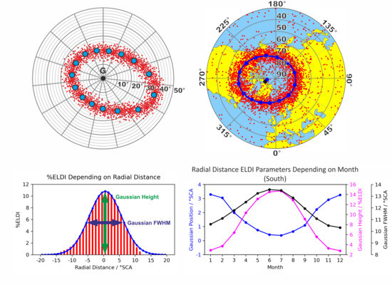
• Next, we created a circle with a radius of 50 °SCA around the geomagnetic pole as center, assuming that it fully covers the auroral region, and divided it into 15 sectors (see Figure 3).
• For every sector we then computed a separate %ELDI histogram depending on the radial distances of the corresponding profiles from the geomagnetic pole. We did this by dividing the sector into 25 bins with a width of 2 °SCA each and subsequently relating in every bin the number of contained ELDI events to the number of profiles.
• To each histogram we then fit a Gaussian function and afterwards estimated the radial distance of its maximum relative to the geomagnetic pole.
• For every sector we subsequently converted this radial distance and the azimuth angle of the sector relative to the geomagnetic pole into a geocentric latitude/longitude contour point of the ellipse. This gave us 15 contour points for all sectors together.
• Finally, we fit an ellipse to the contour points, simultaneously estimating its focal points $\overrightarrow{f_1}$ and $\overrightarrow{f_2}$ and its semimajor axis $a$ by means of least squares fitting. During this process, the following cost function $S_{Ellipse}$, as defined by Mayer and Jakowski [1] in a similar form, was minimized:

  $$S_{Ellipse}=\frac{1}{2}{\displaystyle \sum }_{i=0}^{15}{\left(\left|\mathrm{acos}\left(\overrightarrow{c_i} ·\overrightarrow{f_1}\right)\right|+ \left|\mathrm{acos}\left(\overrightarrow{c_i} ·\overrightarrow{f_2}\right)\right|-2a\right)}^2$$

  (4)

  where
  $\overrightarrow{c_i}$: vector from Earth center to ith contour point/km
  $\overrightarrow{f_1}$: vector from Earth center to first focal point/km
  $\overrightarrow{f_2}$: vector from Earth center to second focal point/km
  $a$: length of semimajor axis/°SCA.

After performing the above procedure separately for both hemispheres, we obtained the reference ellipses as shown in Figure 4A for the northern hemisphere and in Figure 4B for the southern hemisphere. The red dots indicate the individual ELDI events, whereas the blue ellipses depict the reference ellipses together with their contour points (blue dots on ellipses) and their center points (blue dots in ellipse centers). The black dots mark the current locations of the geomagnetic poles as predicted by the IGRF-13 model and provided by the World Data Center for Geomagnetism in Kyoto [17]. It is interesting to note that the positions of the geomagnetic pole and the center point are much closer at the northern pole than at the southern pole area. This observation needs further investigation.

3.1.2. Generation of Radial Distance ELDI Parameters

After determining the reference ellipses, we could compute the values of the radial distance ELDI parameters for any profile subset under consideration by performing the following steps:

• From their geographic latitude/longitude locations we first computed for all profiles their signed radial distance to the corresponding reference ellipse. In this context, a negative sign denotes profiles located poleward, whereas a positive sign denotes profiles located equatorward of the ellipse.
• Next, we created a %ELDI histogram depending on these radial distances. The histogram covered a distance ranging from −20 °SCA to +20 °SCA and consisted of 40 bins with a width of 1 °SCA each.
• We subsequently smoothed the histogram by means of a running average using a 10-bin-wide window. After smoothing, the histogram showed basically a Gaussian shape for any geophysical condition.
• The histogram was still overlaid by background noise caused by profiles that were misclassified as ELDI events, such as sporadic E events. In contrast to the ELDI, these events are characterized by thin, small patches of high ionization in the E layer [18,19]. The fewer real ELDI events occur, as is the case in local summer, the more they are masked by the noise in the histogram. In order to mitigate the influence of the noise and to uncover the Gaussian shape of the histogram for the subsequent fitting step, we first subtracted a fixed noise value of 1% from each histogram bin. In this respect, we manually estimated the noise value from visual inspection of many histograms. Then, starting from the bin containing the largest %ELDI value, we searched for the first empty bin in the direction of decreasing and increasing radial distances. Next, we set all bins outside of these two empty bins to zero.
• After that we fit the histogram with a Gaussian function by means of least squares fitting, simultaneously estimating the values of its parameters $h_{rad}$, ${\mu }_{rad},$ and ${\sigma }_{rad}$. Here we used the following equation for the Gaussian:

  $$b_{rad}{}_i=h_{rad}·{\mathrm{e}}^{-0.5 ·{\left(\frac{r_i-{\mu }_{rad}}{{\sigma }_{rad}}\right)}^2}$$

  (5)

  where
  $b_{rad}{}_i$: value of the ith histogram bin/%ELDI
  $r_i$: radial distance of the ith histogram bin/°SCA
  $h_{rad}$: Gaussian height/%ELDI
  ${\mu }_{rad}$: Gaussian position/°SCA
  ${\sigma }_{rad}$: Gaussian variance/°SCA.

Finally, we converted the Gaussian variance ${\sigma }_{rad}$ into the corresponding full width at half maximum $FWH{M}_{rad}$ using the following formula:

$$FWH{M}_{rad}=2·\sqrt{2·\ln \left(2\right)}·{\sigma }_{rad}$$

(6)

The Gaussian height $h_{rad}$, position ${\mu }_{rad},$ and full width at half maximum $FWH{M}_{rad}$ resulted in the radial distance ELDI parameters of the currently regarded ELDI event distribution. Figure 5A shows the spatial distribution of ELDI events for the northern hemisphere for the $F10.7$ interval from 78.2 to 85.9 SFU as an example. Figure 5B shows the corresponding %ELDI histogram depending on the radial distances together with the fitted Gaussian function. In this example, the Gaussian position is about 0.5 °SCA, whereas its height is about 10% and its FWHM is about 11 °SCA.

3.2. Local Time ELDI Parameter

In this section we explain how we computed the local time ELDI parameter to describe the temporal distribution of a currently regarded subset of ELDI events. Having the development of a user-friendly model of ELDI behavior in view, we focus on local time dependencies instead of using magnetic local time (MLT), being aware that the physics of the related processes is not described in an optimal way. A more detailed discussion of ELDI events in relation to high latitude processes in the thermosphere–ionosphere–magnetosphere system considering MLT dependencies is planned to be performed in a separate study. To retrieve the local time ELDI parameter, we proceeded as follows:

• First, we computed a %ELDI histogram depending on the local time of the profiles. In this context, we divided the range of local times into 48 bins, each one being 0.5 h wide.
• As with the radial distance %ELDI histograms, we also smoothed the local time %ELDI histogram by means of a running average using a 10-bin-wide window.
• We found that for many geophysical conditions the corresponding local time %ELDI histogram was skewed or showed several local maxima. This effect may be explained by different precipitation mechanisms that manifest themselves in different types of auroras at different local times, such as discrete or diffuse auroras [20,21,22]. Due to its asymmetry, the approximation of the histogram by a Gaussian function was not justified. Instead, we determined the local time ELDI parameter ${\mu }_{lt}$, which is the mean local time weighted by %ELDI, as a representative for the entire histogram. Since local times repeat cyclically, for each histogram bin we first converted its local time $l{t}_i$into an angle and then into a unit vector, whose two components we then weighted by the %ELDI value $b_i$of the bin (Equation (7a)). Subsequently, we separately summed up the resulting vector components $x_i$ and $y_i$ for all bins to get the components $x_{sum}$ and $y_{sum}$ (Equation (7b)). Finally, we converted both components into the mean local time ${\mu }_{lt}$using the atan2 function (Equation (7c)).

  $$\left(\begin{array}{c}{x}_i\\ y_i\end{array}\right)=\left(\begin{array}{c}{b}_i·\cos \left(\frac{2\pi }{24}·l{t}_i\right)\\ b_i·\sin \left(\frac{2\pi }{24}·l{t}_i\right)\end{array}\right)$$

  (7a)

  $$\left(\begin{array}{c}{x}_{sum}\\ y_{sum}\end{array}\right)=\left(\begin{array}{c}{\displaystyle \sum }_{i=1}^{48}{x}_i\\ {\displaystyle \sum }_{i=1}^{48}{y}_i\end{array}\right)$$

  (7b)

  $${\mu }_{lt}=\frac{24}{2\pi }·atan2\left(y_{sum},x_{sum}\right)$$

  (7c)

Figure 6 shows the smoothed local time %ELDI histogram for April at the southern hemisphere as an example. The mean local time of this histogram (blue line) has a value of about 0.8.

In the next section we consider how we derived trends of the ELDI parameters depending on the season or geophysical quantities.

3.3. ELDI Parameter Trends

For any given subset of profiles, we computed the values of the ELDI parameters as explained in the previous sections. In order to compute trends of these parameters as a function of the season or geophysical quantities, we performed the steps as shown below. Figure 7 illustrates the steps for the radial distance ELDI parameters as a function of $F10.7$ as an example.

• To generate the ELDI parameter trends depending on a regarded geophysical quantity (as opposed to seasonal dependency), we first established a cumulative histogram of the number of profiles as a function of that quantity. Based on this histogram, we then divided the value range of the quantity into 10 intervals of variable size in such a way that each one contained approximately the same number of profiles.
• As abscissa values of the trends, we subsequently determined for each interval its median value, which divides the interval into two parts, each part containing approximately the same number of profiles.
• Every interval corresponds to a subset of the profiles, which is in turn associated with a certain distribution of ELDI events. For this distribution we computed the four ELDI parameters (Gaussian position, height and FWHM and mean local time) as introduced in the previous sections. These values give the ordinate values of the trends (Figure 7A,B).
• To eliminate outliers and obtain clear trends, we smoothed the original trends by means of a running average using a window width of 5 data points (Figure 7C,D).
• The trends of the individual ELDI parameters depending on any geophysical quantity (as opposed to seasonal dependency) turned out to be similar for the northern and southern hemispheres. Therefore, in this case, we finally computed the average of corresponding trends derived separately for the northern and southern hemispheres (Figure 7E).

4. Results and Discussion

In this section we study the trends of the ELDI parameters as a function of the season and selected geophysical quantities. The plots are organized into two panels each (exceptionally four panels for seasonal dependency). The panels on the left side show the trends of the radial distance ELDI parameters, whereas the panels on the right side show the trend of the local time ELDI parameter. As explained in Section 3, before computing any ELDI parameter values, we first generated a fixed reference ellipse for each hemisphere. For a geophysical condition under consideration, we then computed a %ELDI histogram based on the radial distances of the associated profiles from the respective reference ellipse. After fitting this histogram with a Gaussian function, we determined its height, FWHM, and position relative to the reference ellipse as the radial distance ELDI parameters for the related geophysical condition. In this context, a positive or negative Gaussian position indicates an equatorward or a poleward shift of the distribution, respectively. An increasing Gaussian height is associated with an increasing number of ELDI events. An increase in the Gaussian FHWM indicates an increase in the width of the elliptical precipitation zone. Furthermore, the mean local time of the ELDI event distribution, which we computed according to Equations (7a)–(7c), indicates the local time around which most events occur.

4.1. Dependency on the Season

In order to investigate the seasonal variation of the ELDI parameters, Figure 8 shows their variation as a function of the month. As can be seen, the trends of all radial distance ELDI parameters follow a strong sinusoidal variation over the course of the year. The Gaussian position has its maximum in local summer, which indicates an equatorward shift of the ELDI event distribution for that season. Contrary to this, both the Gaussian FWHM and height are largest in local winter and smallest in local summer. Since the trend of the Gaussian height represents the one for the number of ELDI events, this observation is in line with the findings of Kamal et al. [5]. In their work the authors observed a sinusoidal variation in %ELDI throughout the year with a maximum in local winter and a minimum in local summer. It is also in line with the findings of Cai et al. [3], who observed a larger number of ELDI events for winter and early spring than for the rest of the year. A possible explanation for this result could be that in local summer the increased amount of solar irradiation causes a high F2 layer ionization. The ionization of the E layer caused by particle precipitation is therefore masked by the stronger F2 layer ionization, resulting in a reduced number of ELDI events. The mean local time moves slightly towards midnight around March and towards the morning hours around October for the northern hemisphere. For the southern hemisphere, the order of these trends seems to be reversed, suggesting that this behavior could be systematic. However, further investigations should be conducted to confirm this observation.

4.2. Dependency on Solar Activity

Figure 9 shows the dependency of the ELDI parameters on $F10.7$, which we used as a measure for the solar activity. We see that with increasing $F10.7$ the Gaussian position increases, indicating a shift of the ELDI event distribution towards lower latitudes. At the same time, both the Gaussian FWHM and height decrease. The decrease in the height, i.e., the number of ELDI events, is consistent with the finding of Kamal et al. [5] that in years with low solar activity %ELDI is high, whereas it is low for years with high solar activity. Likewise, when investigating their CHAMP dataset, Mayer and Jakowski [1] found that the number of ELDI events increased in the case of low solar activity. In analogy to the seasonal variation of ELDI occurrence, these observations can be explained by the varying intensity of solar irradiance. In summer, the increased extreme ultraviolet radiation, for which $F10.7$ is a proxy [23], causes increased ionization of the F2 layer. Consequently, this hides the ionization of the E layer, resulting in fewer ELDI occurrences. The trend of the mean local time varies only little for the entire range of $F10.7$.

4.3. Dependency on Geomagnetic Activity

In this section we investigate the dependency of the ELDI parameters on geomagnetic activity, for which we use the $Dst$ index and the $AE$ index as proxies. While the $Dst$ index depends on the strength of the equatorial ring current [24], the $AE$ index is an indicator of the auroral electrojet strength [25]. Both currents and thus both indices are expressions of geomagnetic storms. Figure 10 shows the behavior of the ELDI parameters depending on the $Dst$ index. As can be seen in the plots, decreasing $Dst$ values (and thus increasing geomagnetic activity) are related to an increase in all radial distance ELDI parameters of the distribution. This indicates both an increase in the number of ELDI events and a shift of the ELDI event distribution towards lower latitudes. Concerning the mean local time, we see a shift towards the morning hours.

In comparison, Figure 11 shows the trends of the ELDI parameters depending on the $AE$ index. We see that starting from an $AE$ value of about 80, increasing $AE$ values (and therefore increasing geomagnetic activity) are accompanied by an increase in all three radial distance ELDI parameters, indicating both an increase in the number of ELDI events and an equatorward shift of the ELDI event distribution. In this case, the number of ELDI events given by the Gaussian height increases significantly with increasing geomagnetic activity from about 3–4 to up to 14–15%. These observations are consistent with the $Dst$ dependency of the radial distance ELDI parameters considered before. Likewise, we see an increase in the mean local time, indicating a shift of the ELDI event distribution towards the morning hours for increasing $AE$ values.

The above results concerning the dependencies of the ELDI parameters on geomagnetic activity are consistent with earlier findings and specify them. For example, Mayer and Jakowski [1] found that in the case of geomagnetic disturbances, both the semimajor axis and the width of the elliptical ELDI event distribution increased. Likewise, using the $Kp$ index as a proxy, Xiong and Lühr [8] observed an equatorward shift and an increase in the width of the auroral oval in the case of geomagnetic disturbances. Regarding our results presented above, the variation in the width of the precipitation zone tends towards the same behavior, but is less pronounced, as can be seen by the Gaussian FWHM plots in Figure 10 and Figure 11. Mannucci et al. [4] and Kamal et al. [5] observed a general increase in the number of ELDI events under disturbed conditions, whereas Kamal et al. [5] also observed a shift of the ELDI event distribution towards lower latitudes in the case of geomagnetic storms. These observations agree quite well with current knowledge of high latitude ionospheric behavior in the course of geomagnetic storms [26,27].

4.4. Dependency on the Interplanetary Magnetic Field

After considering the relationships between the ELDI parameters and the geomagnetic indices, it suggests itself to study their dependencies on solar wind observables that drive numerous space weather phenomena, such as geomagnetic storms. In this regard, in Figure 12 we show the ELDI parameters depending on the $Bz$ component of the IMF. In the case of negative $Bz$, the IMF is oriented southwards, indicating a strong impact due to reconnection with the geomagnetic field [28,29,30]. Consequently, for negative $Bz$ values we expect similar results as obtained for growing $AE$ values and negative $Dst$ values, as described in the previous section. As can be seen in the case of a southward oriented IMF, increasing $Bz$ values correlate with an increasing Gaussian position and thus with an equatorward shift of the ELDI event distribution. Furthermore, we observe an increase in the Gaussian FWHM and height for increasingly negative $Bz$ values, indicating an increase in the number of ELDI events during geomagnetic storms. This result agrees quite well with our discussion in the previous section. The trend of the mean local time is similar to that of the Gaussian position, showing a slight increase towards the morning hours with intensification of the southward oriented $Bz$ component of the IMF.

4.5. Dependency on the Convection Electric Field

Since the convection electric field is a key parameter of the solar wind impact on the magnetosphere–ionosphere currents and ionospheric plasma drifts [31,32], we also selected this quantity for studying the characteristics of the ELDI parameters. Figure 13 shows the variation of the ELDI parameters depending on the magnitude $E_{conv}$ of the convection electric field as defined in Equation (2). We see that for increasing $E_{conv}$, the Gaussian position also increases, indicating an equatorward shift of the ELDI event distribution. While the Gaussian FWHM is nearly unchanged, its height shows a steady increase, indicating a rise in the number of ELDI events. As can be seen, with increasing convection electric field magnitude the mean local time also increases, indicating a shift of the ELDI event distribution towards the morning hours. When taking into account that an enhanced convection electric field magnitude corresponds to increased geomagnetic activity and negative $Bz$ values, these dependencies agree quite well with our results considered in the previous Section 4.3 and Section 4.4.

4.6. Dependency on Solar Wind Energy

For estimating the energy input due to the solar wind, we use the proton energy as defined in Equation (1). In this context, energetic protons contribute directly to ELDI events by enhanced ionization in the lower ionosphere. As in the previous sections, we expect a similar dependency of increasing proton energy with increasing convection electric field, negative $Bz,$ and geomagnetic indices. Figure 14 shows the associated trends of the ELDI parameters. For increasing proton energy, the Gaussian position and height increase, indicating an equatorward shift of the ELDI event distribution and an increase in the number of ELDI events. It is obvious that higher energies of solar wind protons will cause an enhanced energy input on the night side via precipitating particles. Therefore, the observed variation of the abovementioned ELDI parameters as a function of the proton energy is not surprising. As in the case of the convection electric field, the Gaussian FWHM is nearly constant, whereas the mean local time shifts towards the morning hours for increasing proton energy.

5. Summary and Conclusions

In the present work we investigate the spatial and temporal variation of E layer dominated ionosphere (ELDI) occurrences depending on various geophysical and space weather-related input quantities, such as seasons, solar activity, geomagnetic activity, interplanetary magnetic field, convection electric field, and solar wind energy. Our observations are based on more than 3.5 million vertical electron density profiles derived from ionospheric GPS radio occultation observations on board the COSMIC/FORMOSAT-3 mission, covering more than one solar cycle from April 2006 to December 2018. The spatiotemporal ELDI event distribution as a function of the above quantities is described by four parameters. In this regard, the spatial distribution of the ELDI events can be approximated by ellipses at the northern and southern polar areas after eliminating the impact of geomagnetic storms. The shape and location of these ellipses is closely related to the geomagnetic poles, but somewhat different for both hemispheres. The derived ELDI parameters characterizing the spatial distribution of the ELDI events are specified in relation to these ellipses as a function of the above input quantities. The temporal distribution of the ELDI events is represented by their mean local time, which varies mostly between 01:00 and 02:00 local time. Regarding the percentage occurrence probability of ELDI events, we see a clear seasonal variation with a maximum in local winter, when the solar irradiation is low. Likewise, ELDI events are more and more suppressed with increasing solar activity due to enhanced extreme ultraviolet ionization in the F2 layer. Considering the other input quantities, the results clearly indicate a higher percentage occurrence probability of up to 15%, guided by an equatorward shift of the ELDI event distribution with increasing values of the solar wind parameters and related geomagnetic activity indices. It should be underlined that all derived dependencies of the ELDI parameters on the input quantities are consistent with each other, indicating that our analysis method is appropriate and reliable. This paves the way for future modeling studies addressing the occurrence and characteristics of ELDI events for applications, particularly in terrestrial and space-based telecommunication and navigation. This application objective is the reason why we describe the temporal distribution of ELDI events with the user-friendly solar local time instead of magnetic local time, which would be closer to the physics of observed dependencies. To get more insight into the underlying physical processes concerning ELDI events, it is planned to consider magnetic local time dependencies of geophysical and space weather-related quantities in detail in future work.

References

1. Mayer, C.; Jakowski, N. Enhanced E-layer ionization in the auroral zones observed by radio occultation measurements onboard CHAMP and Formosat-3/COSMIC. Ann. Geophys. 2009, 27, 1207–1212. [Google Scholar] [CrossRef]
2. Reigber, C.; Lühr, H.; Schwintzer, P.; Wickert, J. Earth Observation with CHAMP: Results from Three Years in Orbit; Springer: Berlin, Germany, 2005; ISBN 978-3-540-26800-0. [Google Scholar]
3. Cai, H.; Li, F.; Shen, G.; Zhan, W.; Zhou, K.; McCrea, I.W.; Ma, S. E layer dominated ionosphere observed by EISCAT/ESR radars during solar minimum. Ann. Geophys. 2014, 32, 1223–1231. [Google Scholar] [CrossRef]
4. Mannucci, A.J.; Tsurutani, B.T.; Verkhoglyadova, O.; Komjathy, A.; Pi, X. Use of radio occultation to probe the high-latitude ionosphere. Atmos. Meas. Tech. 2015, 8, 2789–2800. [Google Scholar] [CrossRef] [Green Version]
5. Kamal, S.; Jakowski, N.; Hoque, M.M.; Wickert, J. Evaluation of E Layer Dominated Ionosphere Events Using COSMIC/FORMOSAT-3 and CHAMP Ionospheric Radio Occultation Data. Remote Sens. 2020, 12, 333. [Google Scholar] [CrossRef] [Green Version]
6. Feldstein, Y.I.; Starkov, G.V. Dynamics of auroral belt and polar geomagnetic disturbances. Planet. Space Sci. 1967, 15, 209–229. [Google Scholar] [CrossRef]
7. Holzworth, R.H.; Meng, C.-I. Mathematical representation of the auroral oval. Geophys. Res. Lett. 1975, 2, 377–380. [Google Scholar] [CrossRef]
8. Carbary, J.F. A Kp-based model of auroral boundaries. Space Weather 2005, 3. [Google Scholar] [CrossRef]
9. Xiong, C.; Lühr, H. An empirical model of the auroral oval derived from CHAMP field-aligned current signatures—Part 2. Ann. Geophys. 2014, 32, 623–631. [Google Scholar] [CrossRef] [Green Version]
10. Newell, P.T.; Sotirelis, T.; Liou, K.; Meng, C.-I.; Rich, F.J. A nearly universal solar wind-magnetosphere coupling function inferred from 10 magnetospheric state variables. J. Geophys. Res. 2007, 112. [Google Scholar] [CrossRef]
11. Anthes, R.A.; Bernhardt, P.A.; Chen, Y.; Cucurull, L.; Dymond, K.F.; Ector, D.; Healy, S.B.; Ho, S.-P.; Hunt, D.C.; Kuo, Y.-H.; et al. The COSMIC/FORMOSAT-3 mission: Early results. Bull. Am. Meteorol. Soc. 2008, 89, 313–333. [Google Scholar] [CrossRef]
12. Rocken, C.; Kuo, Y.-H.; Schreiner, W.S.; Hunt, D.; Sokolovskiy, S.; McCormick, C. COSMIC system description. Terr. Atmos. Ocean. Sci. 2000, 11, 21–52. [Google Scholar] [CrossRef] [Green Version]
13. Liou, Y.-A.; Pavelyev, A.G.; Liu, S.-F.; Pavelyev, A.A.; Yen, N.; Huang, C.-Y.; Fong, C.-J. FORMOSAT-3/COSMIC GPS Radio Occultation Mission: Preliminary Results. IEEE Trans. Geosci. Remote Sens. 2007, 45, 3813–3826. [Google Scholar] [CrossRef]
14. CDAAC. COSMIC Data Analysis and Archive Center. Available online: https://cdaac-www.cosmic.ucar.edu/ (accessed on 15 December 2020).
15. SPDF. OMNIWeb Service. Available online: https://omniweb.gsfc.nasa.gov/ (accessed on 15 December 2020).
16. Kelley, M.C. The Earth's Ionosphere: Plasma Physics and Electrodynamics, 2nd ed.; Academic Press: Cambridge, MA, USA, 2009; Volume 96, ISBN 978-0120884254. [Google Scholar]
17. WDC. Magnetic North, Geomagnetic and Magnetic Poles. Available online: http://wdc.kugi.kyoto-u.ac.jp/poles/polesexp.html (accessed on 15 December 2020).
18. Arras, C.; Wickert, J. Estimation of ionospheric sporadic E intensities from GPS radio occultation. J. Atmos. Sol.-Terr. Phys. 2018, 171, 60–63. [Google Scholar] [CrossRef]
19. Wu, D.L.; Ao, C.O.; Hajj, G.A.; de la Torre Juarez, M.; Mannucci, A.J. Sporadic E morphology from GPS-CHAMP radio occultation. J. Geophys. Res. 2005, 110. [Google Scholar] [CrossRef] [Green Version]
20. Akasofu, S.I. Recent progress in studies of DMSP auroral photographs. Space Sci. Rev. 1976, 19, 169–215. [Google Scholar] [CrossRef]
21. Lui, A.T.Y.; Perreault, P.; Akasofu, S.-I.; Anger, C.D. The diffuse aurora. Planet. Space Sci. 1973, 21, 857–861. [Google Scholar] [CrossRef]
22. Lui, A.T.Y.; Anger, C.D. A uniform belt of diffuse auroral emission seen by the ISIS-2 scanning photometer. Planet. Space Sci. 1973, 21, 799–809. [Google Scholar] [CrossRef]
23. Doherty, P.H.; Klobuchar, J.A.; Kunches, J.M. Eye on the Ionosphere: The Correlation between Solar 10.7 cm Radio Flux and Ionospheric Range Delay. GPS Solut. 2000, 3, 75–79. [Google Scholar] [CrossRef]
24. Sugiura, M. Hourly values of equatorial Dst for the IGY. In Annals of the International Geophysical Year; Pergamon Press: Oxford, UK, 1964; Volume 35, pp. 7–45. [Google Scholar]
25. Davis, T.N.; Sugiura, M. Auroral electrojet activity index AE and its universal time variations. J. Geophys. Res. 1966, 71, 785–801. [Google Scholar] [CrossRef] [Green Version]
26. Milan, S.E.; Hutchinson, J.; Boakes, P.D.; Hubert, B. Influences on the radius of the auroral oval. Ann. Geophys. 2009, 27, 2913–2924. [Google Scholar] [CrossRef] [Green Version]
27. Yokoyama, N.; Kamide, Y.; Miyaoka, H. The size of the auroral belt during magnetic storms. Ann. Geophys. 1998, 16, 566–573. [Google Scholar] [CrossRef]
28. Gonzalez, W.D.; Joselyn, J.A.; Kamide, Y.; Kroehl, H.W.; Rostoker, G.; Tsurutani, B.T.; Vasyliunas, V.M. What is a geomagnetic storm? J. Geophys. Res. 1994, 99, 5771–5792. [Google Scholar] [CrossRef]
29. Gonzalez, W.D.; Tsurutani, B.T.; Clúa de Gonzalez, A.L. Interplanetary origin of geomagnetic storms. Space Sci. Rev. 1999, 88, 529–562. [Google Scholar] [CrossRef]
30. Dungey, J.W. Interplanetary Magnetic Field and the Auroral Zones. Phys. Rev. Lett. 1961, 6, 47–48. [Google Scholar] [CrossRef]
31. Baumjohann, W.; Blanc, M.; Fedorov, A.; Glassmeier, K.-H. Current Systems in Planetary Magnetospheres and Ionospheres. Space Sci. Rev. 2010, 152, 99–134. [Google Scholar] [CrossRef]
32. Milan, S.E.; Clausen, L.B.N.; Coxon, J.C.; Carter, J.A.; Walach, M.-T.; Laundal, K.; Østgaard, N.; Tenfjord, P.; Reistad, J.; Snekvik, K.; et al. Overview of Solar Wind–Magnetosphere–Ionosphere–Atmosphere Coupling and the Generation of Magnetospheric Currents. Space Sci. Rev. 2017, 206, 547–573. [Google Scholar] [CrossRef]
Figure 1. (A) Number of vertical electron density profiles derived from COSMIC (Constellation Observing System for Meteorology, Ionosphere, and Climate) radio occultation observations depending on the year and (B) number of profiles depending on the geographic latitude.
Remotesensing 12 04109 g001
Figure 2. (A) Average solar radio flux index F 10.7 depending on the year, (B) number of observed profiles related to F 10.7 , and (C) seasonal distribution of the number of profiles.
Remotesensing 12 04109 g002
Figure 3. Contour point generation. The E layer dominated ionosphere (ELDI) events (red dots) are distributed around the geomagnetic pole G. After constructing a circle with a radius of 50 degrees spherical central angle around the pole, dividing it into 15 sectors (straight grey lines), and dividing each of them into 25 bins (grey circles), we computed one contour point (blue dots) for each sector.
Remotesensing 12 04109 g003
Figure 4. (A) ELDI event distribution (red dots) for geomagnetic quiet conditions together with reference ellipse (blue ellipse), contour points (blue dots on ellipse), center point (blue dot in center of ellipse), and geomagnetic pole (black dot) for the northern hemisphere and (B) for the southern hemisphere.
Remotesensing 12 04109 g004
Figure 5. (A) ELDI event distribution (red dots) with reference ellipse (blue ellipse) for the F 10.7 interval from 78.2 to 85.9 SFU for the northern hemisphere and (B) corresponding histogram (red bars) of the percentage of ELDI events (%ELDI) depending on the radial distance with fitted Gaussian function (blue curve) and indications of the Gaussian height (green arrow) and of its full width at half maximum (FWHM) represented by a blue arrow.
Remotesensing 12 04109 g005
Figure 6. Local time %ELDI histogram for April at the southern hemisphere with indication of the mean local time (blue line).
Remotesensing 12 04109 g006
Figure 7. Radial distance ELDI parameter trends as a function of F 10.7 . (A,B) Original parameter trends for the northern and southern hemispheres, (C,D) smoothed parameter trends, and (E) parameter trends averaged over both hemispheres.
Remotesensing 12 04109 g007
Figure 8. ELDI parameter trends depending on the month. (A,C) Radial distance ELDI parameters and (B,D) local time ELDI parameter.
Remotesensing 12 04109 g008
Figure 9. ELDI parameter trends depending on F 10.7 . (A) Radial distance ELDI parameters and (B) local time ELDI parameter.
Remotesensing 12 04109 g009
Figure 10. ELDI parameter trends depending on the disturbance storm time index D s t . (A) Radial distance ELDI parameters and (B) local time ELDI parameter.
Remotesensing 12 04109 g010
Figure 11. ELDI parameter trends depending on the auroral electrojet index A E . (A) Radial distance ELDI parameters and (B) local time ELDI parameter.
Remotesensing 12 04109 g011
Figure 12. ELDI parameter trends depending on the component B z of the interplanetary magnetic field. (A) Radial distance ELDI parameters and (B) local time ELDI parameter.
Remotesensing 12 04109 g012
Figure 13. ELDI parameter trends depending on the magnitude E c o n v of the convection electric field. (A) Radial distance ELDI parameters and (B) local time ELDI parameter.
Remotesensing 12 04109 g013
Figure 14. ELDI parameter trends depending on the proton energy W p r o t . (A) Radial distance ELDI parameters and (B) local time ELDI parameter.
Remotesensing 12 04109 g014
Publisher’s Note: MDPI stays neutral with regard to jurisdictional claims in published maps and institutional affiliations.