Abstract
The spatial fragmentation of high-resolution remote sensing images makes the segmentation algorithm put forward a strong demand for noise immunity. However, the stronger the noise immunity, the more serious the loss of detailed information, which easily leads to the neglect of effective characteristics. In view of the difficulty of balancing the noise immunity and effective characteristic retention, an adaptive distance-weighted Voronoi tessellation technology is proposed for remote sensing image segmentation. The distance between pixels and seed points in Voronoi tessellation is established by the adaptive weighting of spatial distance and spectral distance. The weight coefficient used to control the influence intensity of spatial distance is defined by a monotone decreasing function. Following the fuzzy clustering framework, a fuzzy segmentation model with Kullback–Leibler (KL) entropy regularization is established by using multivariate Gaussian distribution to describe the spectral characteristics and Markov Random Field (MRF) to consider the neighborhood effect of sub-regions. Finally, a series of parameter optimization schemes are designed according to parameter characteristics to obtain the optimal segmentation results. The proposed algorithm is validated on many multispectral remote sensing images with five comparing algorithms by qualitative and quantitative analysis. A large number of experiments show that the proposed algorithm can overcome the complex noise as well as better ensure effective characteristics.
1. Introduction
Image segmentation plays a crucial role in remote sensing image interpretation, segmentation accuracy can directly affect the quality of interpretation [1]. The goal of image segmentation is to partition the image into a group of homogeneous regions, and the features in the homogeneous region are highly similar [2]. With the development of the spatial resolution of remote sensors, the high-spatial-resolution remote sensing images provide rich surface features. However, the fine spatial structure also increases the heterogeneity of homogeneous regions and complicates the spatial correlation. These characteristics bring big challenges to high-accuracy remote sensing image segmentation in balancing the noise immunity and effective characteristic retention [3,4].
At present, the commonly used segmentation methods include watershed [5,6], level set [7,8], clustering [9,10], and so on. In watershed methods, the image is regarded as landforms and the gray as altitude. The segmentation results are obtained by the boundary of the basin according to the lowest altitude. It can detect the weak boundary, but it is also easy to cause over-segmentation. The basic idea of the level set is to express the plane closed curve implicitly as the level set of two-dimensional surface function and achieve segmentation by the evolution of the level set function. However, it is sensitive to gradient information. Clustering methods gather pixels with similar features to complete segmentation. It is simple and easy to implement, and widely studied in remote sensing image segmentation. According to the basic processing unit, the clustering algorithm can be divided into two types, pixel-based [11,12] and region-based [13,14]. The pixel-based algorithms, even the popular fuzzy C-means (FCM) algorithm which integrates the fuzzy set theory, are susceptible to outliers [15]. To improve the robustness, a series of segmentation algorithms with spatial constraints is proposed. Modified FCM (FCM_S) [16] added a regularization term defined by the dissimilarity between neighborhood pixels and clusters. However, noise immunity is only slightly improved. Enhanced FCM (EnFCM) [17] and Fast Generalized FCM (FGFCM)[18] built a weighted image based on the spectra of neighboring pixels and executed segmentation based on the grayscale. The segmentation accuracy increased, but the segmentation boundaries usually have a certain error with the real [19]. Fuzzy Local Information C-Means (FLICM) [20] and Reformulated FLICM (RFLICM) [21] defined the local fuzzy factor described by the spatial distance and the local variation coefficient of central pixel respectively. Although the noise immunity is improved obviously, there are still a lot of mis-segmented pixels [22]. In the statistical framework, on the basis of using probability distribution to describe the random characteristics of the spectra to reduce sensitivity, Markov Random Fields (MRF) is also utilized to establish the prior probability based on the neighborhood system to further enhance the robustness [23]. Chatzis and Varvarigou [24] integrated the statistical model into the fuzzy structure and proposed Hidden Markov Random Field FCM (HMRF_FCM). The Gaussian distribution is used instead of Euclidean distance to model dissimilarity between pixels and clusters. The KL entropy regularization term is established by the prior probability based on MRF. Although HMRF-FCM has achieved great success, the robustness is still not insufficient because of the pixel-based processing [25]. Nowadays, region-based methods have become an inevitable trend of image segmentation due to the good performance in smoothing noise and the advantage of describing local characteristics [26,27].
There are two key issues on region-based segmentation methods [28], (1) how to generate the sub-regions, (2) how to realize segmentation based on sub-regions. For the first issue, the most commonly used algorithm is the Simple Linear Iterative Clustering (SLIC) [29,30] in superpixel algorithms [31,32]. The sub-regions are generated by assigning pixels to the nearest seed points, where the dissimilarity measure between pixels and seed points is modeled by combing spatial and spectral distance with scale parameters. For the second issue, the general way is to cluster sub-regions with similar characteristics [33]. For example, Yang et al. [34] proposed a local spectral angle as the similarity measure to merge the adjacent sub-regions. Zhou et al. [35] extracted spectral, shape, and texture features to represent the characteristics of sub-regions for describing the similarity. Lei et al. [36] proposed a superpixel-based fast fuzzy c-means clustering algorithm (SF_FCM). The sub-regions generated by multi-scale morphological gradient reconstruction watershed transform are clustered according to the histogram. However, traditional region-based methods must execute clustering operations based on optimal sub-regions results. The state of sub-regions cannot be adjusted adaptively according to the current segmentation result, which leads to a great dependence of segmentation results on sub-region results. The Voronoi-based segmentation algorithm proposed by Li.et al. [37] fortunately can solve this problem. Taking the spatial distance as the dissimilarity between pixels and seed point, the image is divided into a group of sub-regions by Voronoi tessellation technology. Based on the Voronoi sub-region, the segmentation models established under the fuzzy clustering framework are studied for remote sensing images [25]. The moving-updating operation of seed points during segmentation provides an effective tool for the adaptive adjustment of the sub-regions state. However, stronger noise immunity is easy to ignore useful detailed information.
To further improve the performance of the region-based segmentation algorithms in preserving effective details, a novel Voronoi tessellation technology with adaptive weighted distance is proposed for remote sensing image segmentation. To divide the image domain into many sub-regions with high spectral homogeneity and spatial connectivity, the distance between pixels and seed points in Voronoi tessellation extends from only spatial information to both spatial and spectral. An adaptive weight coefficient, modeled by a monotone decreasing function, is designed to control the spatial connectivity. After dividing, the dissimilarity between Voronoi sub-regions and clusters is modeled by the negative logarithm of the Gaussian probability distribution function (pdf) to further accurately describe the cluster characteristics. To consider the effect of spatial neighborhood system, the prior probability in Kullback–Leibler (KL) entropy regularization is defined based on MRF theory. Then, the optimal segmentation result is obtained by solving the segmentation model parameters according to parameter characteristics. The main contributions of this paper are summarized as follows,
- (1)
- We design a monotone decreasing function as the adaptive weight coefficient to control the influence intensity of spatial information. The farther the spatial distance is, the more important the spectral information is. Therefore, both the spectral homogeneity and spatial connectivity of sub-regions can be ensured greatly.
- (2)
- Integrating the adaptive distance-weighted Voronoi tessellation into the fuzzy clustering framework can describe the segmentation uncertainty more effectively and better balance the noise immunity and effective characteristic retention.
This paper is organized as follows. In Section 2 the adaptive distance-weighted Voronoi tessellation is introduced first, and then the establishing and solving of the regionalized segmentation model are discussed in detail. In Section 3, the experiments are designed to demonstrate the effectiveness of the proposed algorithm qualitatively and quantitatively. In Section 4, a deep analysis of the performance of the proposed algorithm is further discussed. Finally, the conclusion is exposed in Section 5.
2. Methods
An image I = {Ii(ai, bi): i = 1, …, n, (ai, bi) ∈ Ω} is formed by giving the spectral information on a finite set of 2-D rectangular discrete pixel lattice Ω = {(ai, bi): i = 1, …, n}; where i and n are the index and the total number of pixels, Ii= (Iie: e = 1, …, h) is the spectral characteristic vector of pixel i, e, and h are the index and the total number of spectral channel, (ai, bi) is lattice position of pixel i, respectively. For dividing the image domain into a series of sub-regions, the seed points set G = {gj(uj, vj): j = 1, …, m, (uj, vj) ∈ Ω} need to be produced first, where j and m are the index and the total number of seed points, gj= (gje: e = 1, …, h) and (uj, vj) are spectral characteristic vector and lattice position of seed point j, respectively. The sub-regions corresponding to seed points can be expressed as V = {Vj: j = 1, …, m}.
2.1. Adaptive Distance-Weighted Voronoi Tessellation
Voronoi tessellation is a spatial tessellation technology that divides the space into several sub-spaces according to the distance between points and seed points. the pixel has not only spatial position information but also spectral characteristic information, thus the distance can be described from two aspects by Equations (1) and (2),
where d[·] represents distance function, and it is usually defined by Euclidean distance, dijs and dijc are the spatial distance and spectral distance between pixel i and seed point j, respectively.
In the traditional Voronoi-based segmentation algorithms, the distance is only modeled based on the spatial distance. Then, the sub-region Vj is obtained by
Although Equation (3) provides a good way for overcoming the complex noise, the spectral information must be considered by model constraints in the segmentation process. This method is deficient in the accurate description of image characteristics.
To consider the comprehensive effect of spatial position and spectral characteristic information in Voronoi tessellation, the mixed distance dij of spatial distance dijs and spectral distance dijc is established. Then, the sub-region Vj is re-obtained by Equations (4) and (5),
where wijs and wijc are the weighted coefficients of spatial distance and spectral distance respectively, they are satisfied wijs + wijc = 1. In order to make full use of the spatial distance to overcome the noise, and to finely describe the image characteristics with the help of spectral information, the adaptive weight coefficient determined by a monotone decreasing function with the increasing spatial distance is constructed by Equation (6),
where Ms is the maximum value of dijs (i∈{1, …, n}, j∈{1, …, m}), α is the adaptive factor, α∈[0,1]. The curve of wijs with different α is shown in Figure 1. It shows that the weight is independent of the spatial distance when α = 0, and the bigger α is, the closer the weight is to 1.
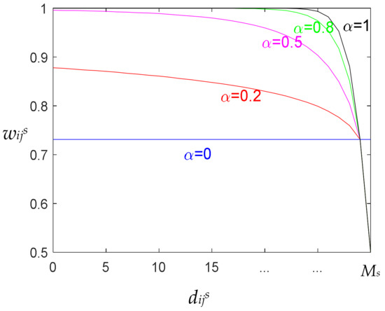
Figure 1.
Weight curve with different α.
In particular, dijs and dijc are in different orders of magnitude, which easily leads to invalid distance. Therefore, a normalization operation is performed according to Equations (7)–(10).
where and are the normalized spatial and spectral distance, ξs and ξc are the corresponding normalization coefficient respectively,
According to Equations (5)–(10), dij can be rewritten as,
where is the maximum value of (i ∈ {1, …, n}, j ∈ {1, …, m}).
The visualization of the spatial distance effect is shown in Figure 2. Figure 2a represents the traditional Voronoi tessellation, Figure 2b represents the adaptive distance-weighted Voronoi Tessellation, where the depth of color represents the intensity of spatial distance effect to the corresponding seed point. It can be seen that pixels in the boundary between two homogeneous regions have smaller spatial distance effects, which can consider more spectral information and help to further accurately describe the image characteristics.
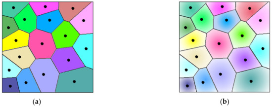
Figure 2.
Visualization of spatial distance effect. (a) Traditional Voronoi tessellation; (b) Adaptive distance-weighted Voronoi Tessellation.
2.2. Segmentation Model
Assume that there are k homogeneous regions in the image, the fuzzy relationship between sub-regions and clusters can be expressed as R = [rjl]m×k, where rjl is fuzzy membership of sub-region Vj belonging to cluster l, and satisfied . Then, the regionalized fuzzy cluster objective function can be defined as,
where sjl is the dissimilarity measure between sub-region Vj and cluster l, λ is the regularization term coefficient used to control the fuzzy degree, is the number of pixels in sub-regions Vj, “#” is the counting symbol, ρjl is the scale factor that protects small-scale cluster from being easily affected by large-scale.
Assuming that the spectra of pixels in sub-region Vj follow independently identically Gaussian distribution, the joint probability of pixels in Vj conditional on Lj = l can be defined as,
where I(j) = {Ii: (ai, bi) ∈ Vj} represents the spectra of sub-region Vj, θ = {μ, Σ} is distribution parameter set, μ = {μl: l = 1, …, k} and Σ = {Σl: l = 1, …, k} are mean and covariance of Gaussian distribution that cluster l follows, L = {Lj: j = 1, …, m }, Lj ∈ {1, …, k} is the cluster label to which sub-region Vj belongs. The lager the dissimilarity measure is, the higher the consistency of features is. Thus, combining Equation (13), sjl can be defined as negative log-likelihood of the probability,
In order to consider the spatial constraints, the positions and cluster labels of pixels can be regarded as a random field that is called the label field. Then, based on MRF, the scale factor can be defined by the prior probability of sub-region Vj belonging to cluster l according to Hammersley-Clifford theorem by Equation (15),
where is the neighborhood system of sub-region Vj, as shown in Figure 3, the pink represents the center sub-region Vj, the green represents the neighbor sub-regions Vj′, “~” represents neighborhood relationship; j′ is the index of neighborhood sub-regions; is the normalization term; c is the index of cliques; C is the clique set; Uc is the potential energy of clique c. In the region-level, C is the binary clique composed of all adjacent sub-regions. Thus, Uc can be defined based on the Potts model,
where β is neighborhood sub-regions interaction intensity, β∈[0, 1].
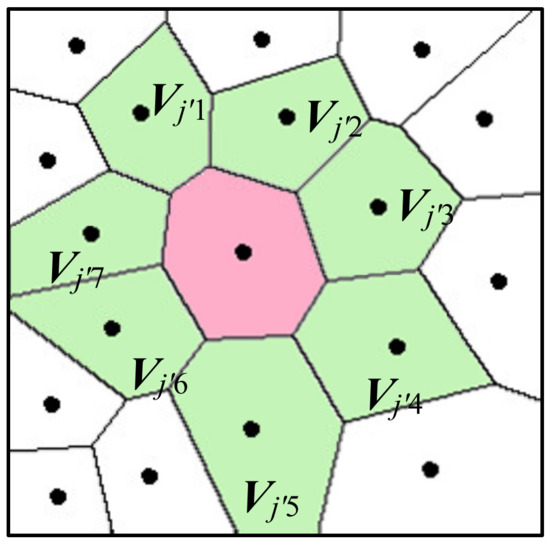
Figure 3.
Neighbor system visual model.
2.3. Parameter Estimation
According to the characteristics of parameters, some applicable solution schemes are designed to obtain the optimal parameter.
(1) For R, it needs to achieve the minimization objective function under the constrain , thus, it is necessary to establish Lagrange function L(R, G, θ) by Equation (17),
where υ = {υj: j = 1, …, m} is Lagrange coefficient. Let , then, rjl can be obtained by eliminating υj,
(2) For θ, the analytical formulas can be obtained directly from derivatives. Let then, μl and Σl can be obtained by Equations (19) and (20),
(3) For G. It is implicitly expressed in the objective function and cannot be solved by derivative. To determine the optimal position of seed points, a special descent method based on the image domain is designed. Suppose that the seed point of sub-region Vj slightly changes its location from the original position (uj, vj) to candidate position (uj, vj) + o(uj, vj), i.e., (uj, vj)*, and all other seed points remain at the same position, where o(uj, vj) represented the descent direction is a minimal moving distance. Let V = {V1, V2, …, Vj, …, Vm} be the sub-regions set generated by the original seed points set G = {g1(u1, v1), g2(u2, v2), …, gj(uj, vj), …, gm(um, vm)} and V* = {V1, V2, …, Vj*, …, Vm} be the candidate sub-regions set generated by the candidate seed points set G* = {g1(u1, v1), g2(u2, v2), …, gj*(uj, vj)*, …, gm(um, vm)}. Owing to the slight moving operation, the sub-regions change slightly. This change occurs only in Vj and its adjacent sub-regions, as shown in Figure 4, where the green represents adjacent sub-regions, the black heavy line area represents Vj, the red heavy line area represents Vj*, the blue represents the newly added area, the yellow represents the discarded area, the purple represents overlapping areas. From this property, the judgment function can be calculated by Equation (21),
where s(il) can be regarded as the dissimilarity between pixel i and cluster l.
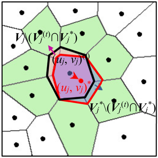
Figure 4.
Solution model of G.
If ΔJ < 0, accept the candidate seed point (uj, vj)*, otherwise, stay at the same.
2.4. Summary of the Proposed Algorithm
The process of the proposed algorithm can be summarized as follows, and the algorithm flow chart is shown in Figure 5.
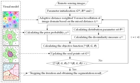
Figure 5.
Flow chart of the proposed algorithm.
S1 Initializing the generating point set G(0) = {gj(0)(uj, vj)(0): j = 1, …, m, (uj, vj)(0) ∈ Ω}, the fuzzy membership R(0) = [rjl(0)]m×k, and the iteration indicator τ = 0;
S2 Calculating the spatial distance dijs(τ) and spectral distance dijc(τ) by Equations (1) and (2);
S3 Calculating the normalized distance and by Equations (7)–(10);
S4 Calculating the mixed distance dij(τ) by Equation (11), and then the Voronoi tessellation of image domain is completed by Equation (4);
S5 Calculating distribution parameter set θ(τ) by Equations (19) and (20), and calculating the dissimilarity measure sjl(τ) by Equations (13) and (14);
S6 Calculating the prior probability ρjl(τ) by Equations (15) and (16);
S7 Calculating fuzzy membership R(τ) by Equation (18);
S8 Calculating the objective function J(τ) (R, G, θ) by Equation (12);
S9 Updating the seed points set G(τ) by Equations (21) and (22);
S10 Repeating S2–S9 until the objective function is minimized, i.e., |J(τ)(R, G, θ) − J(τ −1)(R, G, θ)| < ε, where ε is a minimal non-negative number.
3. Experimental Results
To verify the effectiveness of the proposed algorithm, the experiments based on the proposed algorithm and five comparing algorithms including FCM_S [16], HMRF_FCM [24], SLIC_FCM [29], SF_FCM [36], VT_HMRF_FCM [25] are carried out on simulated image and multispectral remote sensing images. The characteristics of these comparing algorithms are listed in Table 1. The simulated image can provide a controllable environment for better evaluation and verification. In addition, the effectiveness of the proposed algorithm is also discussed by qualitative and quantitative evaluation, respectively.

Table 1.
The characteristics of comparing algorithms.
3.1. Simulated Image
Figure 6a is the simulated image generated by the template with distribution parameters, as shown in Figure 6b and Table 2, where I-V are five homogeneous regions representing grass, water, forest, road, and artificial surface, respectively. There are similar means in regions I and III, the similar standard deviation in regions I and II, the sharp boundary between regions I and II, and slender geometry-shape in region IV.
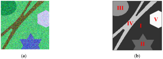
Figure 6.
Simulated image and template. (a) Simulated image; (b) Template with five homogeneous regions.
Table 2.
Gaussian distribution parameters for generating the simulated image.
Figure 7 is the representative segmentation result of the simulated image, where the three in the column represent segmentation results, outline images of segmentation regions, and superposition images of outline and simulated image, as shown in Figure 7a1–a3, the six in the row represent FCM_S, HMRF_FCM, SLIC_FCM, SF_FCM, VT_HMRF_FCM, and the proposed algorithm, as shown in Figure 7a1–f1. It can be seen that the speckle noise is unavoidable in the segmentation results based on pixel-based algorithms, as shown in Figure 7a1–a3,b1–b3. SLIC_FCM can effectively solve the speckle noise, but it cannot effectively distinguish the boundaries between homogeneous regions with similar spectra and segment the slender roads, as shown in Figure 7c1–c3. For SF_FCM, the boundary is eroded, especially in regions II and IV, as shown in Figure 7d1–d3. VT_HMRF_FCM greatly improves the smoothness and accuracy of the segmentation boundary, but it fails in the slender road, as shown in Figure 7e1–e3. For the proposed algorithm, it cannot only solve the problem of mis-segmentation of regions with similar spectra, but also realize the effective segmentation of the slender road, as shown in Figure 7f1–f3.
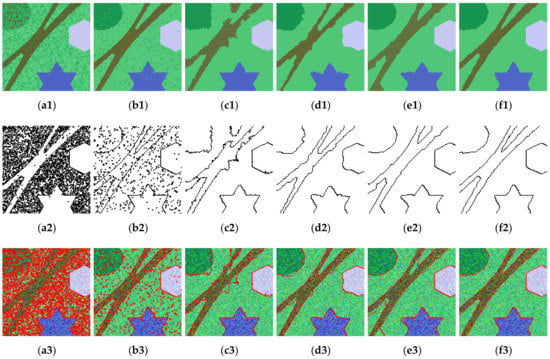
Figure 7.
Representative segmentation results of simulated image. (a1–a3) FCM_S; (b1–b3) HMRF_FCM; (c1–c3) SLIC_FCM; (d1–d3) SF_FCM; (e1–e3) VT_HMRF_FCM; (f1–f3) The proposed algorithm.
To analyze the quality of sub-regions, the fitting deviation of sub-regions to homogeneous regions are shown in Figure 8. Figure 8a1–d1 are the sub-regions results of SLIC_FCM, SF-FCM, VT_HMRF_FCM and the proposed algorithm respectively, Figure 8a2–d2 shows the corresponding fitting deviation image, Figure 8a3–d3 shows the detail views. In Figure 8a1–a3, the sub-regions of SCLIC_FCM always cross the boundaries of homogeneous regions because the fixed weight used to integrate spatial and spectral information is easy to make the spectral information not giving full play. In Figure 8b1–b3, due to the neglect mechanism of gradient details, the boundaries of the sub-regions deviate from that of the homogeneous regions. In Figure 8c1–c3, although the phenomenon of sub-regions crossing the boundary of homogeneous regions has been partially improved by optimizing the location of the seed points, it is still not accurate enough on the slender road. In Figure 8d1–d3, the sub-regions generated by the adaptive distance-weighted Voronoi tessellation can fit the boundary of the homogeneous regions smoothly and accurately.
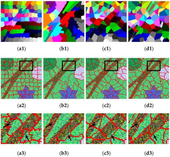
Figure 8.
Visualization of the quality of sub-regions. (a1–a3) SLIC_FCM; (b1–b3) SF_FCM; (c1–c3) VT_HMRF_FCM; (d1–d3) The proposed algorithm.
To quantitatively evaluate the effectiveness of the proposed algorithm, the User’s Accuracy (UA), Producer’s Accuracy (PA), Overall Accuracy(OA), and Kappa coefficient (Kappa) are calculated based on the confusion matrix built by segmentation results and template, as shown in Table 3. It shows that FCM_S is at the lowest accuracy, the OA and Kappa are only 74.48% and 0.63, respectively. Those of HMRF_FCM are 95.85% and 0.93 respectively, which is mainly influenced by the UA of region III. The OA of the three region-based algorithms, SLIC_FCM, SF_FCM, and VT_HMRF_FCM, are all above 96%, Kappas are also above 0.93. For the proposed algorithm, the OA and Kappa are 98.90% and 0.98, which is much higher than the algorithms mentioned above.
Table 3.
Quantitative evaluation of simulated image segmentation results.
3.2. Remote Sensing Image Segmentation
To verify the segmentation effect for multispectral remote sensing images, many different types of images are tested with the proposed algorithm and five comparing algorithms, where the representative images are selected and shown in Figure 9. Figure 9a1–d1 represents slender geometric features, different features with similar spectral characteristics, the same features with different spectral characteristics, features with high spatial fragmentation, respectively. Figure 9a1,c1 is 128 × 128 and 256 × 256 pixels from WorldView−2 images with 0.5 resolution, Figure 9b1,d1 is 128 × 128 and 256 × 256 pixels from IKONOS images with 1 resolution. Figure 9a2–d2 shows the template images corresponding to Figure 9a1–d1, I-V represent different homogeneous regions.
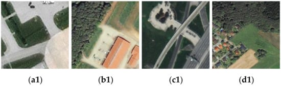
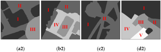
Figure 9.
Multispectral remote sensing images. (a1–d1) Images 1–4; (a2–d2) The corresponding templates.
Figure 10 is the representative segmentation result of multispectral remote sensing images. From left to right, the six columns represent FCM_S, HMRF_FCM, SLIC_FCM, SF_FCM, VT_HMRF_FCM, and the proposed algorithm, respectively. FCM_S usually makes a big mis-segmentation, such as regions II and III in Figure 10a1, and exists many speckle noise, such as region I in Figure 10a2 and region IV in Figure 10a4. Although HMRF_FCM has greatly improved the confusion phenomenon because of the advantage of the statistical model, there is still a lot of segmentation noise, especially for the region with a big variance, as shown in Figure 10b4. For SLIC_FCM, the segmentation noise is solved, but the results have a high under segmentation rate, such as region III in Figure 10c2 and region II in Figure 10c3. SF_FCM is good at segmenting homogeneous regions and difficult to overcome heterogeneous elements in regions with a big variance, as shown in the comparison between Figure 10d1,d4. VT_HMRFC_FCM has a strong ability to overcome heterogeneity, but it is easy to ignore the positive details, such as the slender road of region II in Figure 10e1 and the gap between houses of region III in Figure 10e2. For the proposed algorithm, it can overcome the heterogeneity while maintaining a great deal of positive information. The slender road, gaps, and the regions with big variance are effectively segmented, as shown in Figure 10f1–f4.
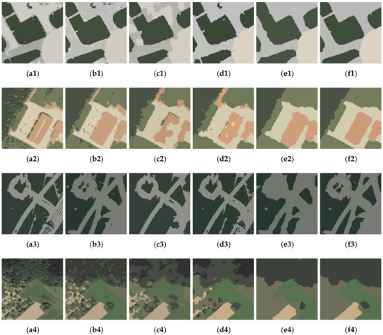
Figure 10.
Segmentation results of multispectral remote sensing images. (a1–a4) FCM_S; (b1–b4) HMRF_FCM; (c1–c4) SLIC_FCM; (d1–d4) SF_FCM; (e1–e4) VT_HMRF_FCM; (f1–f4) The proposed algorithm.
Table 4 is the quantitative evaluation of multispectral remote sensing image segmentation results. It shows that the highest OA and Kappa of FCM_S are only 83.26% and 0.77, respectively. The accuracy of HMRF_FCM is higher than SLIC_FCM, but less than SF_FCM, such as Figure 9a1,d1. For Figure 9a1, SF_FCM and VT_HMRF_FCM have similar accuracy. But for the images with strong heterogeneity, SF_FCM is much lower than VT_HMRF_FCM, such as Figure 9d1. However, the accuracy of the proposed algorithm is always the highest one, the OA and Kappa can be as high as 98.23% and 0.97, respectively.
Table 4.
Quantitative evaluation of multispectral remote sensing images segmentation results.
4. Discussion
To study the proposed algorithm deeply, the parameters influence and comprehensive performance are further discussed in this section, where the number of sub-regions m can control the fineness of the segmentation, the regularized term coefficient λ controls the fuzzy degree of clustering, the neighborhood sub-regions interaction intensity β determines the degree of spatial constrain, and the adaptive factor α is used to balance the weight of spatial and spectral information. In addition, OA is used as the evaluation criteria.
4.1. Parameter Influence Analysis
The influence of different model parameters on segmentation results is discussed by the control variate method, as shown in Figure 11. Figure 11a–d represent m, λ, β, and α respectively. Figure 11a shows that the OA increases from rapid to slow with the increased m, but the running time increases steadily. The bigger the m is, the more updating of seed points is needed. According to segmentation efficiency, it can be seen that the best value range of m is 80–100. It can achieve higher accuracy in less time. Figure 11b illustrates that λ has little effect on segmentation results in the range of 0.1–0.7. In Figure 11c, the OA drops sharply from 0.7, and the highest value is at 0.3. In Figure 11d, OA shows a decreasing trend from 0.2. Generally, the best value of α is about 0.2.
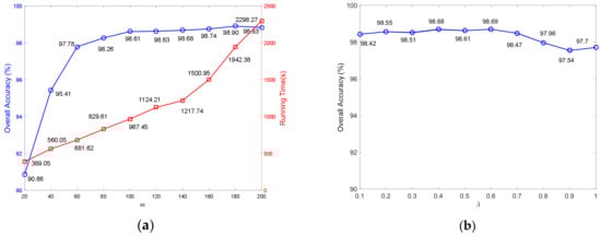
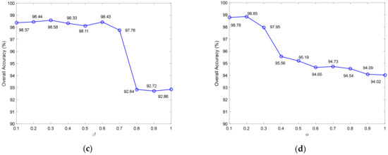
Figure 11.
Influence analysis of different model parameters. (a) m; (b) λ; (c) β; (d) α.
4.2. Comprehensive Performance Analysis
Figure 12 is the box-plot for multispectral remote sensing image segmentation results, which is used to evaluate the comprehensive performance of algorithms. The dotted line covers the range of OA. The box shows the range of centralized data. The red line represents the median. Figure 12a–d corresponds to Figure 9a1–d1, respectively. It shows that HMRF_FCM, SLIC_FCM, SF_FCM, and VT_HMRF_FCM have different degrees of instability in segmenting different types of images, FCM_S is stable at a relatively low level, the proposed algorithm is stable at a high level and always above 90%. Besides, the greater the variance of the image, the more obvious the advantage of the proposed algorithm, as shown in Figure 12d.
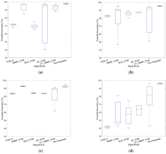
Figure 12.
Box-plot of the overall accuracy of multispectral remote sensing images segmentation results based on the proposed and comparing algorithms. (a–d) represent images 1–4.
5. Conclusions
In this study, an adaptive distance-weighted Voronoi tessellation is proposed to deal with the difficulty of balancing the noise immunity and effective characteristic retention in remote sensing image segmentation. The monotone decreasing function is designed to describe the weight for coupling spatial distance and spectral distance in Voronoi tessellation, which provides a new technique for ensuring the spectral homogeneity and spatial connectivity of sub-regions as much as possible. The pdf of Gaussian distribution used to model dissimilarity can effectively describe the random distribution characteristics of spectra. The Voronoi sub-regions-based fuzzy clustering objective function established by KL entropy regularization term based on MRF model not only can accurately model the segmentation uncertainty, but also effectively model the spatial neighborhood effect at sub-region level. Besides, the parameter solving methods are designed according to the characteristics, which can greatly approach the optimal solution.
A large number of experiments show that the proposed algorithm can keep effective detail information while keeping high noise immunity. The segmentation accuracy is significantly improved, especially for the images with large spectral variance and great differences of cluster scale. However, there are still some limitations, one is that the number of Voronoi sub-regions needs to be determined according to the empirical knowledge, another is that the unimodal distribution cannot effectively describe the multimodal distribution caused by complexed scene. To solve these limitations, the initialization method of the number of sub-regions and modeling method based on multimodal distribution can be further studied.
Author Contributions
This research was mainly performed by X.L. and J.C. X.L. contributed with ideas, conceived, and designed the study, J.C. supervised the study and his comments were considered throughout the paper. L.Z., S.G., L.S., and X.Z. aided in proposing the idea, giving suggestions, and revising the rough draft. All authors have read and agreed to the published version of the manuscript.
Funding
This research was funded by the Strategic Priority Research Program of the Chinese Academy of Sciences, grant number XDA19030301, and the National Natural Science Foundation of China, grant number (42001286, 41801360, 41771403, 41801358).
Acknowledgments
Thanks to the anonymous reviewers for their constructive and valuable suggestions on the earlier drafts of this manuscript.
Conflicts of Interest
The authors declare that they have no conflict of interest.
References
- Troyagalvis, A.; Gancarski, P.; Passat, N.; Bertiequille, L. Unsupervised quantification of under- and over-segmentation for object-based remote sensing image analysis. IEEE J. Sel. Topics Appl. Earth Obs. Remote Sens. 2015, 8, 1936–1945. [Google Scholar] [CrossRef]
- Peng, B.; Zhang, L.; Zhang, D. Automatic image segmentation by dynamic region merging. IEEE Trans. Image Process. 2011, 20, 3592–3605. [Google Scholar] [CrossRef]
- Zhao, J.; Zhong, Y.; Shu, H.; Zhang, L. High-resolution image classification integrating spectral-spatial-location cues by conditional random fields. IEEE Trans. Image Process. 2016, 25, 4033–4045. [Google Scholar] [CrossRef]
- Chen, B.; Qiu, F.; Wu, B.; Du, H. Image segmentation based on constrained spectral variance difference and edge penalty. Remote Sens. 2015, 7, 5980–6004. [Google Scholar] [CrossRef]
- Ciecholewski, M. River channel segmentation in polarimetric SAR images: Watershed transform combined with average contrast maximisation. Expert Syst. Appl. 2017, 82, 196–215. [Google Scholar] [CrossRef]
- Cousty, J.; Bertrand, G.; Najman, L.; Couprie, M. Watershed cuts: Thinnings, shortest path forests, and topological watersheds. IEEE Trans. Pattern Anal. Mach. Intell. 2010, 32, 925–939. [Google Scholar] [CrossRef] [PubMed]
- Braga, A.M.; Marques, R.C.P.; Rodrigues, F.A.A.; Medeiros, F.N.S. A median regularized level set for hierarchical segmentation of SAR images. IEEE Geosci. Remote Sens. Lett. 2017, 14, 1171–1175. [Google Scholar] [CrossRef]
- Jin, R.; Yin, J.; Zhou, W.; Yang, J. Level set segmentation algorithm for high-resolution polarimetric SAR images based on a heterogeneous clutter model. IEEE J. Sel. Topics Appl. Earth Obs. Remote Sens. 2017, 10, 4565–4579. [Google Scholar] [CrossRef]
- Mao, T.; Tang, H.; Huang, W. Unsupervised classification of multispectral images embedded with a segmentation of panchromatic images using localized clusters. IEEE Trans. Geosci. Remote Sens. 2019, 57, 8732–8744. [Google Scholar] [CrossRef]
- Fan, J.; Wang, J. A two-phase fuzzy clustering algorithm based on neurodynamic optimization with its application for PolSAR image segmentation. IEEE Trans. Fuzzy Syst. 2018, 26, 72–83. [Google Scholar] [CrossRef]
- Gu, H.; Han, Y.; Yang, Y.; Li, H.; Liu, Z.; Soergel, U.; Blaschke, T.; Cui, S. An efficient parallel multi-scale segmentation method for remote sensing imagery. Remote Sens. 2018, 10, 590. [Google Scholar] [CrossRef]
- Yuan, J.; Wang, D.; Li, R. Remote sensing image segmentation by combining spectral and texture features. IEEE Trans. Geosci. Remote Sens. 2014, 52, 16–24. [Google Scholar] [CrossRef]
- Arisoy, S.; Kayabol, K. Mixture-based superpixel segmentation and classification of SAR images. IEEE Geosci. Remote Sens. Lett. 2016, 13, 1721–1725. [Google Scholar] [CrossRef]
- Qin, X.; Zou, H.; Zhou, S.; Ji, K. Region-based classification of SAR images using Kullback–Leibler distance between generalized Gamma distributions. IEEE Geosci. Remote Sens. Lett. 2015, 12, 1655–1659. [Google Scholar]
- Toro, C.; Martín, C.; Pedrero, A.; Ruiz, E. Superpixel-based roughness measure for multispectral satellite image segmentation. Remote Sens. 2015, 7, 14620–14645. [Google Scholar] [CrossRef]
- Ahmed, M.N.; Yamany, S.M.; Mohamed, N.A.; Farag, A.A.; Moriarty, T.M. A modified fuzzy c-means algorithm for bias field estimation and segmentation of MRI data. IEEE Trans. Med. Imag. 2002, 21, 193–199. [Google Scholar] [CrossRef]
- Szilagyi, L.; Benyo, Z.; Szilagyi, S.M.; Adam, H.S. MR brain image segmentation using an enhanced fuzzy C-means algorithm. In Proceedings of the 25th Annual International Conference of the IEEE Engineering in Medicine and Biology Society, Cancun, Mexico, 17–21 September 2003; pp. 724–726. [Google Scholar]
- Cai, W.; Chen, S.; Zhang, D. Fast and robust fuzzy c-means clustering algorithms incorporating local information for image segmentation. Pattern Recognit. 2007, 40, 825–838. [Google Scholar] [CrossRef]
- Zhang, H.; Bruzzone, L.; Shi, W.; Hao, M.; Wang, Y. Enhanced spatially constrained remotely sensed imagery classification using a fuzzy local double neighborhood information C-means clustering algorithm. IEEE J. Sel. Topics Appl. Earth Obs. Remote Sens. 2018, 11, 2896–2910. [Google Scholar] [CrossRef]
- Krinidis, S.; Chatzis, V. A robust fuzzy local information C-means clustering algorithm. IEEE Trans. Image Process. 2010, 19, 1328–1337. [Google Scholar] [CrossRef]
- Gong, M.; Zhou, Z.; Ma, J. Change detection in synthetic aperture radar images based on image fusion and fuzzy clustering. IEEE Trans. Image Process. 2012, 21, 2141–2151. [Google Scholar] [CrossRef]
- Memon, K.H.; Lee, D. Generalised kernel weighted fuzzy C-means clustering algorithm with local information. Fuzzy Sets Syst. 2018, 340, 91–108. [Google Scholar] [CrossRef]
- Zhang, H.; Wang, Q.; Shi, W.; Hao, M. A novel adaptive fuzzy local information C-means clustering algorithm for remotely sensed imagery classification. IEEE Trans. Geosci. Remote Sens. 2017, 55, 5057–5068. [Google Scholar] [CrossRef]
- Chatzis, S.P.; Varvarigou, T. A fuzzy clustering approach toward hidden Markov random field models for enhanced spatially constrained image segmentation. IEEE Trans. Fuzzy Syst. 2008, 16, 1351–1361. [Google Scholar] [CrossRef]
- Zhao, Q.; Li, X.; Li, Y.; Zhao, X. A fuzzy clustering image segmentation algorithm based on Hidden Markov Random Field models and Voronoi Tessellation. Pattern Recognit. Lett. 2017, 85, 49–55. [Google Scholar] [CrossRef]
- Blaschke, T. Object based image analysis for remote sensing. ISPRS J. Photogramm. Remote Sens. 2010, 65, 2–16. [Google Scholar] [CrossRef]
- Zhang, X.; Xiao, P.; Feng, X. Object-specific optimization of hierarchical multiscale segmentations for high-spatial resolution remote sensing images. ISPRS J. Photogramm. Remote Sens. 2020, 159, 308–321. [Google Scholar] [CrossRef]
- Su, T. Scale-variable region-merging for high resolution remote sensing image segmentation. ISPRS J. Photogramm. Remote Sens. 2019, 147, 319–334. [Google Scholar] [CrossRef]
- Achanta, R.; Shaji, A.; Smith, K.; Lucchi, A.; Fua, P.; Susstrunk, S. SLIC superpixels compared to state-of-the-art superpixel methods. IEEE Trans. Pattern Anal. Mach. Intell. 2012, 34, 2274–2282. [Google Scholar] [CrossRef]
- Pan, X.; Zhou, Y.; Chen, Z.; Zhang, C. Texture relative superpixel generation with adaptive parameters. IEEE Trans. Multimedia. 2019, 21, 1997–2011. [Google Scholar] [CrossRef]
- Lang, F.; Yang, J.; Yan, S.; Qin, F. Superpixel segmentation of polarimetric SAR image using generalized mean shift. Remote Sens. 2018, 10, 1592. [Google Scholar] [CrossRef]
- Stutz, D.; Hermans, A.; Leibe, B. Superpixels: An evaluation of the state-of-the-art. Comput. Vis. Image Und. 2018, 166, 1–27. [Google Scholar] [CrossRef]
- Zhang, Y.; Wang, X.; Tan, H.; Xu, C.; Ma, X.; Xu, T. Region merging method for remote sensing spectral image aided by inter-segment and boundary homogeneities. Remote Sens. 2019, 11, 1414. [Google Scholar] [CrossRef]
- Yang, J.; He, Y.; Caspersen, J.P. Region merging using local spectral angle thresholds: A more accurate method for hybrid segmentation of remote sensing images. Remote Sens. Environ. 2017, 190, 137–148. [Google Scholar] [CrossRef]
- Zhou, Y.; Chen, Y.; Feng, L.; Zhang, X.; Shen, Z.; Zhou, X. Supervised and adaptive feature weighting for object-based classification on satellite images. IEEE J. Sel. Top. Appl. Earth Obs. Remote Sens. 2018, 11, 3224–3234. [Google Scholar] [CrossRef]
- Lei, T.; Jia, X.; Zhang, Y.; Liu, S.; Meng, H.; Nandi, A.K. Superpixel-based fast fuzzy C-means clustering for color image segmentation. IEEE Trans. Fuzzy Syst. 2019, 27, 1753–1766. [Google Scholar] [CrossRef]
- Li, Y.; Li, J.; Chapman, M.A. Segmentation of SAR intensity imagery with a Voronoi tessellation, bayesian inference, and reversible jump MCMC algorithm. IEEE Trans. Geosci. Remote Sens. 2010, 48, 1872–1881. [Google Scholar] [CrossRef]


Publisher’s Note: MDPI stays neutral with regard to jurisdictional claims in published maps and institutional affiliations. |
© 2020 by the authors. Licensee MDPI, Basel, Switzerland. This article is an open access article distributed under the terms and conditions of the Creative Commons Attribution (CC BY) license (http://creativecommons.org/licenses/by/4.0/).