Abstract
This paper introduces a new method to analyze the positional accuracy of georeferenced satellite images without the use of ground control points. Compared to the traditional method used to carry out this kind of analysis, our approach provides a semiautomatic way to obtain a larger number of control points that satisfy the requirements of current standards regarding the size of the set of sample points, the positional accuracy of such points, the distance between points, and the distribution of points in the sample. Our methodology exploits high quality orthoimages, such as those provided by the Aerial Orthography National Plan (PNOA)—developed by the Spanish National Geographic Institute—and has been tested on spatial data from Landsat 8. Our method works under the current international standard (ASPRS 2014) and exhibits similar performance than other well-known methods to analyze the positional accuracy of georeferenced images based on the use of independent ground control points. More specifically, the positional accuracy achieved for a Landsat 8 dataset evaluated by the traditional method is 5.22 ± 1.95 m, and when evaluated with the proposed method, it exhibits a typical accuracy of 5.76 ± 0.50 m. Our experimental results confirm that the method is equally effective and less expensive than other available methods to analyze the positional accuracy of satellite images.
1. Introduction
Remote sensing (RS) and geographical information systems (GIS) are playing an increasingly significant role in Earth science and related disciplines and their applications, including land cover mapping [1], precision agriculture [2], biodiversity [3], climate [4], snow-glacier monitoring, terrestrial temperature, erosion, flood monitoring, ocean coast monitoring, and biodiversity [5]. Decision support systems (DSS) can also be used to enhance water usage, decrease air pollution and define sustainable urban development [6]. Whatever the area of application, the outcome will strongly depend on the positional accuracy of the data. Accordingly, RS, GIS, and DSS must provide tools to precisely determine the degree of accuracy, resolution, and integrity of positional data [7].
A geo-referenced image includes an additional data set for each pixel p in the image, which contains a pair of xy-coordinates with terrestrial information about the location of that particular pixel. Taking into account that the geometric resolution of the image defines the pixel size, the geo-referencing process guarantees that each xy-coordinate pair is always inside the limits of the corresponding pixel.
To correctly use a geo-referenced image (for example, to obtain distances), the user needs to have a previous idea of the accuracy of the results. The positional accuracy measures the reliability of the xy-coordinates with regard to a prevailing projected geodetic reference system [8]. In this sense, there are studies that consider the evaluation of the positional accuracy of a georeferenced image as a fundamental part of the analysis, and it can be expressed as a comparison between the values of the xy-coordinates and the true values, or those that we accept as such [9]. Most importantly, in order to assess the positional accuracy of spatial data, the geographic projection system control points must conform a set with independent, easily identifiable, and recognizable coordinates. Accordingly, the process of evaluating the positional accuracy of spatial images comprises the collection of a set of xy-coordinate pairs from a reliable source, along with the identification of a set of pixels in the image and the associated xy-coordinate pairs set . The final results are obtained by computing statistics obtained from the distances between each pair of homologous points in and .
Consistent with the way in which the control point coordinates are obtained and how they are identified in the image, the points that are selected to carry out the positional accuracy evaluation are named independent control points (ICP). In this paper, we refer to those points that have been obtained in the “ground” by means of differential global positioning systems (DGPS) as independent ground control points (IGCPs). In our context, the term ICP will be used to denote control points obtained from highly accurate geo-referenced ortho-images.
The process of selecting the set of points that may be used to assess the positional accuracy of a spatial image must follow certain constraints. In this regard, the American Society for Photogrammetry and Remote Sensing (ASPRS) [10] standard recommends the use of a source of more precise data as a starting point. Specifically, it is recommended that the accuracy of the control data should be at least three times the accuracy of the analyzed data. To this end, traditional methods use a set of IGCPs as the reference source, whose accuracy is mainly measured in centimeters [11,12,13]. This approach, however, presents important drawbacks. First, the control points must be directly collected on the ground, which is usually very costly. Moreover, in rugged terrains, accessing the selected points may be difficult or even impossible. Last but not least, the lack of DGPS signal coverage in urban areas or in areas with high vegetation may completely preclude the positional accuracy evaluation. Therefore, obtaining these IGCPs is not always a simple task and, as a result, few control points are frequently used in traditional methods to perform the positional accuracy analysis.
There are recent studies related to this area of knowledge that show that the interest of the community in evaluating data quality control methods is really alive. Some of the more recent ones are related to the positional quality and current standards [14]. Other works investigate methods based on thematic quality [15,16]. Last but not least, there are also examples of quality control studies related to Building Information Modelling (BIM) datasets [17].
In this paper, we introduce a new method to analyze the positional accuracy of georeferenced satellite images without the use of ground control points. Our method exhibits similar performance than other well-known methods to analyze the positional accuracy of georeferenced images based on the use of IGCPs, but with less computational demands.
2. Related Works
Due to the relevance of positional accuracy in georeferenced satellite images, some official committees have published guidelines for selecting a minimum number of ICPs, and the recommended statistics to present the results [8]. The problem of low-quality positional accuracy in studies based on satellite and aerial imagery is well known [7,9]. Comparisons of topographic maps and GPS-derived points were performed for the geometric correction of SPOT and Landsat [7].
The number of ICPs required for satellite imagery correction was derived in [18] from a function with different parameters: collection method, type and resolution of the sensor, image spacing, geometric model, study site, physical environment, definition, and the accuracy of GCPs versus the final expected accuracy. In [19], an approach for the automatic registration of geo-located Landsat 8 Operational Land Imager (OLI) data is reported, but the positional quality is evaluated only visually. The evaluation of the geometric accuracy of high-resolution satellite images (HRSIs) has been increasingly studied in recent years.
Table 1 summarizes relevant examples of studies where the positional accuracy of geo-referenced data is evaluated, and the number of ICPs used is reported. The first column of the table depicts the study date. The title of the work and the sensor used are specified in the second column. The third column includes a reference of the work. The last column indicates the number of IGCPs used in the positional accuracy evaluation and the source of their corresponding coordinates (when available).

Table 1.
Relevant works analyzing the positional accuracy of satellite images.
In all these analyses, the accuracy of the estimation of the digital elevation model grows with the number of control points [20,21]. On the other hand, the users of satellite imagery can find some guidelines on the geometric quality control of the corrected product in [22] and the Spanish Standard UNE 148002 [23]. An overview of the 2015 ASPRS positional accuracy standards for digital geospatial data is presented in [22].
3. Main Contribution
The increasing existence and availability of very well-positioned spatial data from aerial ortho-images (and from images taken by unmanned aerial vehicles) allows their fusion with georeferenced satellite images, opening new opportunities for assessing spatial resolution, also known as ground sample distance (GSD) (measurement in the field of pixels). Statistical parameters can be used to compare the differences in the coordinates of the center of pixels in satellite images with other images with greater accuracy (and better GSD) by obtaining a positional evaluation of the already geo-referenced spatial data.
The GSD is the linear dimension of the footprint of one pixel on the ground in the source image [28], and the “pixel size” is assumed to be the size of a pixel on the terrain in a digital image, after all rectifications and resampling procedures have been performed. In addition, in the most widely used standards (such as ASPRS), GSD belongs to horizontal and non-oblique images, as GSD values can vary greatly in cities and mountainous areas [10].
There is a large amount of freely available data sets from geo-referenced remote sensing images, from high-resolution spatial images which, combined with the large amount of geomatic data with high positional accuracy (e.g., orthoimages with high accuracy), can be used to determine the positional accuracy of the analyzed remote sensing data.
In this paper, we introduce a reliable semiautomatic method in which the positional accuracy of the georeferenced satellite image can be performed without using IGCPs. This is done by obtaining ICPs from freely available and highly accurate orthoimages. Our method overcomes the main drawbacks previously described in the classical procedure to assess the positional accuracy of satellite images. The new method uses a variation of the Poisson–Disc Sampling algorithm (PDS), which provides control points with uniform distribution and minimum distance [29]. We adapted the Bridson algorithm to finally guarantee the compliance with well-established standards. An experimental study has been conducted in this work to validate the reliability of the proposed method as compared to traditional approaches.
4. Materials and Study Area
The spatial data used in this work consists of a satellite image, whose positional accuracy is to be analyzed, and the high-resolution control image from which the checkpoints (ICPs) will be obtained to evaluate the positional quality of the satellite image.
4.1. Spatial Image to Be Analyzed
The satellite image used in the study was collected by Landsat 8 and its spatial resolution is 15 meters in its panchromatic band. Each scene is composed of 11 GeoTIFF files, one per spectral band, a metadata file (MTL), and one additional file with scene quality assessment (QA) information. The analyzed images belong to band 8 (the panchromatic band), since it has better spatial resolution than the rest of the bands. Each image corresponds to a surface of approximately 180 km from North to South and 190 km from East to West (From now on, zone extension will be expressed as n × m with n representing vertical dimension and m indicating horizontal dimension.), and the images have been obtained from an orbital flight with height of 705 km. The image used in the experiment was collected on 15 September 2018. The analyzed spatial image was downloaded into WGS84. The technical information of the images used in the evaluation is summarized in Table 2.
Table 2.
Summary of technical data of images used for the analysis of positional accuracy.
4.2. Positional Control Data
The IGCPs (points whose coordinates have centimetric precision) have been obtained using DGPS and will be used to validate the proposed method. The set of IGCPs available in this study belongs to the Geodesic Polygonal Network of Cáceres, and comprise 102 points distributed through the urbanized area of the municipality of Cáceres.
In addition, we use as control image an orthoimage made available by the Aerial Orthography National Plan of Spain (PNOA). The orthoimages of PNOA are georeferenced images with different resolutions, but those used in this study have a resolution of 25 cm and a planimetric accuracy of ±50 cm. The PNOA ortho-images used as control data were carried out from a DEM obtained by a LiDAR methodology, with a mesh size of 5 × 5 m and positional accuracy with root mean square error (RMSE) of 2 m. These orthoimages have been obtained using photogrammetric flights equipped with high-resolution digital cameras, multispectral sensors, and panchromatic sensors. PNOA ortho-images can be downloaded from the National Center for Geographic Information (CNIG) of the National Geographic Institute (IGN) in Spain (https://pnoa.ign.es/). The images are of raster type with ECW (Enhanced Compression Wavelet) format, and have a size of approximately 2 GB. The map extension is approximately 20 × 30 km. The orthoimages used for positional control have ETRS89 Reference System, and the map projection is UTM 29 and 30 N (EPSG: 25830). Table 3 gives information about the control points used in the tests.
Table 3.
Summary of control data used for the analysis of positional accuracy.
4.3. Study Area
We refer to the study area (SA) as the specific rectangular region in the satellite image whose positional accuracy we want to analyze. In this work, the SA is located in the municipality of Cáceres, Spain, and it corresponds to an administrative zone enclosing the urbanizing area of the city, with a real extension of 7.6 × 7.8 km. Figure 1a,b depict the corresponding satellite image and the SA inside it.
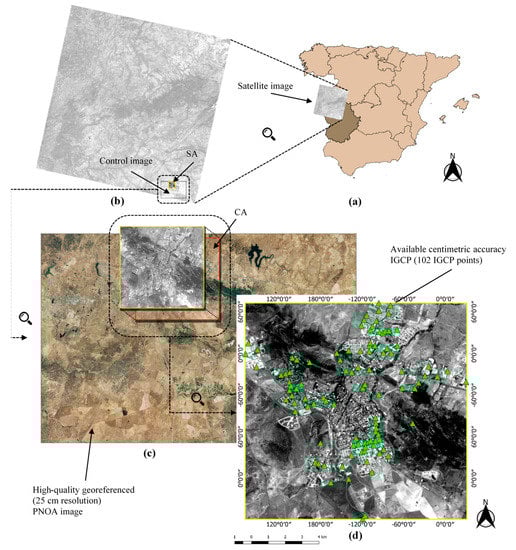
Figure 1.
(a) Geographical location of the study area in Spain, in the province of Cáceres, Extremadura. (b) Landsat 8 image (in grey), PNOA orthoimage (gray dotted line), and the study area (SA, yellow framed). (c) Zoom of the PNOA ortho-image (gray dotted line) with the selected CA (red framed) inside of it. (d) Zoom of the SA under study with indication of the existing IGCPs (green triangles) from the Geodesic Polygonal Network of Cáceres.
4.4. Control Area
Once the SA has been defined, one or more control images covering the SA must be identified. Indeed, these control images must exhibit a high-quality level of georeferencing so they can be used to obtain reliable ICPs. As we stated before, we use PNOA ortho-images for this purpose. In our case, only one PNOA control image (with an extension of 20 × 30 km) is enough to cover the considered SA. The area delimited by the control image is marked with a gray dotted line in Figure 1b. Figure 1c shows the PNOA control image. We assign the control area (CA) to the rectangular section identified in the control image corresponding to the SA, which is also depicted in Figure 1c. Note that the SA (belonging to the satellite image) and the CA (belonging to the control image) cover the same extension, but comprise different resolutions. Figure 1d shows, just as a reference, the location of the 102 available IGCPs inside the SA, although the position of IGCP points inside the CA may involve certain inaccuracies because the IGCPs have centimetric resolution and our PNOA image has one-fourth meter resolution.
5. Proposed Methodology
The goal of our method is to provide a semiautomatic way to carry out the positional accuracy analysis of a zone of interest (SA) in a georeferenced satellite image. The key point in this analysis is to achieve a representative sample of checkpoints that are able to infer reliable conclusions about the positional quality of the georeferenced satellite image. However, the collection of these samples is very hard and time consuming, while crucial to the process. In the traditional methods, the sample consists of a set of IGCPs that must be manually obtained, so that usually there is just one chance (if any) to carefully select a representative sample. Our method overcomes this difficulty by offering a virtually unlimited number of different samples to carry out the statistical analysis to derive the positional accuracy of the georeferenced image or, more precisely, the SA.
As stated, our method uses ICPs instead of IGCPs. In the evaluation of the quality of geographical data, the ASPRS standard [10] provides two main recommendations about the used ICPs:
- (ASPRSa) Depending on the area extension under study, there must be a minimum number of checkpoints to be used in the evaluation process. A table with the minimum values for different region extensions can be obtained from [10].
- (ASPRSb) The accuracy of ICPs used must be at least three times more than the SA accuracy.
Another important point with regards to the quality of the positional accuracy analysis process has to do with the recommendations made by the Spanish Association for Standardization and Certification (AENOR) [23] regarding the distribution of the ICPs. According to AENOR, the ICP sample must satisfy the following conditions:
- (AENORa) Each individual checkpoint must be at a minimum distance from any other point greater than (or equal to) one tenth of the diagonal of the SA.
- (AENORb) By splitting the SA in four quadrants, each one must contain at least 20% of the total number of selected checkpoints.
To be reliable, spatial accuracy analysis must comply with the previous requirements, so that all of them are required conditions for our method. Our proposal meets both the ASPRS and AENOR requirements.
Figure 2 presents a graphical description of our algorithm. Figure 3 shows one of the distributions generated by our PDS (Figure 3a,b), and a graphical example illustrating the identification and correlation of ICPs in the CA. The satellite image and the high-resolution ortho-image constitute the input data for the process. From them, the SA and CA sub-images are extracted, having both the same land extension. To comply with the ASPRSb requirement, the CA planimetric positional accuracy from which we will extract the ICPs must be at least three times finer than the SA planimetric positional accuracy.
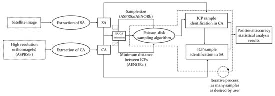
Figure 2.
Algorithm of the proposed method. The central core of the method is the application of the PDS algorithm to obtain well-distributed samples.
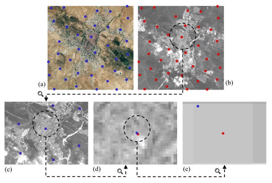
Figure 3.
Graphical example of the proposed automatic method, with a homogeneous and random distribution and correlation of a PDS sample with 39 ICPs. (a) SA PNOA with 39 ICPs (blue circles) automatically generated and randomly distributed using PDS. (b) CA Landsat 8 with 39 ICPs (red circles) identified through the PNOA ICPs using the process in Figure 2. (c) Zoom of Figure 3b. (d) Zoom of Figure 3c, showing the location of the SA ICPs (blue circle) and the ICP identified on CA (red circle). (e) Figure representing a pixel on CA where the ICP is located. The blue circle represents the SA ICP and the red circle represents the CA ICP (center of pixel), identified through the method proposed (in Figure 2).
Because we are using PNOA images with a spatial resolution of 25 cm and ±0.50 m of planimetric positional accuracy, and bearing in mind that the Landsat image has spatial resolution of 15 m, with planimetric positional accuracy that can be considered approximately half of the pixel (7.5 m), we can ensure ASPRSb compliance (0.50 < 7.5 m/3). It is precisely the land extensions that provide the input parameters to the PDS algorithm that finally obtains the ICP sample.
PDS is an efficient algorithm for providing a uniform non-clustered random sample of points inside a region. The algorithm takes as input two parameters: (i) the extent (width and length) of the sample domain (the SA/CA extension) and (ii) the minimum distance between sample individuals. Both parameters can be obtained directly from the SA/CA extension, because the minimum distance is calculated as one tenth of the SA/CA diagonal extension (by ensuring the AENORa requirement). The PDS algorithm has been adapted to guarantee the compliance of requirements ASPRSa and AENORb. The output of PDS is a sample of n points in a rectangle of a virtually infinite resolution. Thus, for this set of raw points to represent an ICP sample set inside the CA image, it must be adjusted to the CA resolution. This process is done in the “ICP sample identification in CA” box in Figure 2, and it involves identifying, for every raw point , the pixel in CA that covers it. From the set of pixels , we finally obtain the corresponding set ICP_CA = of xy-coordinate pairs (These xy-coordinates pairs are specifically the center of pixels. Note that images are given in the visual spectrum, so that the shortest reference for a human eye is the pixel itself. As a result, we take the center as the representative of each pixel.) (remember that the CA is a georeferenced image), which becomes the ICP sample set. Now, the accuracy of the ICP_CA points is ±50 cm.
Once we have obtained the ICP_CA sample set, we apply a similar adjustment procedure to identify the corresponding points in the SA. Specifically, for every in ICP_CA, the pixel in the SA that covers it is identified, and its associated is obtained by creating the homologous ICP_SA = set. In this case, the ICP_SA points resolution is ±15 m.
Figure 2 shows that the PDS algorithm can be executed a number of times to obtain as many samples as needed, thereby improving the degree of reliability of the positional accuracy analysis results.
The last step of the method is to analyze the positional accuracy of SA through a collection of statistics calculated on the set of Euclidean distances for every pair of corresponding points in ICP_CA and ICP_SA.
6. Results
To validate the proposed methodology, we compare the results of the positional accuracy evaluation of the chosen SA (described in Section 4) using a traditional method and our method.
6.1. Analysis of Positional Accuracy Following the Traditional Method
The evaluation of the positional accuracy of an SA (according to traditional methods) requires the existence of a set of control points, usually obtained in a manual way by using a GPS device (IGCPs). In our case, the council of Cáceres has provided us with a set of 102 IGCPs distributed on the SA. By using this set of IGCPs, we have applied a modified version of the PDS algorithm to extract a representative and uniformly distributed sample meeting the ASPRS (Actually, the ASPRSa standard cannot be satisfied just by one point because of the particular distribution available IGCP points.) and AENOR standards. This sample consists of 19 IGCP control points, IGCP_Sample = .
Once the IGCP_Sample set has been selected, the next step is to identify, in the SA image, the corresponding set of xy-coordinates pairs IGCP_SA = by following the procedure described in Section 5.
Finally, Euclidean distances are calculated to present the main statistical measures, namely, the mean , the standard deviation , the maximum , and the minimum . All of the statistical measures are given in meters. This value is generally presented as RMSE, but we prefer to use the standard deviation by considering the analysis values as distances (not errors). Taking into account that points in IGCP_Sample have centimetric precision, all the previous values are in a confidence range of ±0.01 m.
6.2. Analysis of Positional Accuracy Using the Proposed Method
As stated in Section 5, the goal of our method is to achieve an alternative set of control points (ICPs) to evaluate the positional accuracy of the SA. Therefore, instead of the IGCP_Sample set, we need to find a relevant ICP_Sample from the CA by following the procedure in Figure 2. Because of the great efficiency of the PSD algorithm, it is easy (and fast) to generate a collection of candidate ICP_Sample sets. Since the PSD algorithm uses a random approach to generate points, different executions of the algorithm will produce different results (in terms of sample size and the position of points) for the same CA. With the aim of getting confident results, we decided to work with a collection of equal sized ICP_Sample sets. A total of 100 PSD runs were performed, each one providing a different ICP_Sample set. Figure 4 depicts the results obtained for the different sample sizes (in number of ICP points). As it can be noted, the largest quantity (30%) of equal-sized samples corresponds to samples containing 39 points, so we finally used these 30 samples of 39 ICP points for our tests. For each ICP_Sample , we obtained the corresponding ICP_SA = by following our method and took the distances to finally estimate the positional accuracy of the SA. Table 4 shows the resulting values for each generated ICP_Sample. Note that, because the used CA image has a resolution of 25 cm, distances have been rounded to the nearest fourth of a meter before obtaining their averages (). The last column in Table 5 summarizes the average values for the means and standard deviations, and it also shows maximum and minimum values for all the samples. All these values must be considered in a confidence range of ±0.50 m.
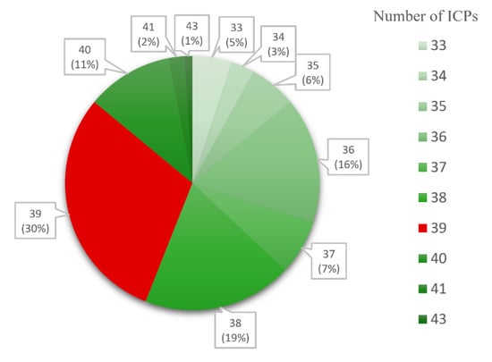
Figure 4.
Quantities and percentages of equal-sized samples obtained in a total of 100 runs of the PDS algorithm.
Table 4.
Summary of the statistics obtained in the 30 samples tested in the proposed method.
Table 5.
Summary of the statistics by comparing the traditional method with the proposed one.
7. Discussion
Conforming to the generally accepted traditional method, the analysis of positional accuracy of the satellite image on the SA selected suggests that the included geo-references have an accuracy of 5.22 m with a standard deviation of ±1.95 m (on a pixel size of 15 m, we can safely disregard the ±0.01 m due to the centimetric accuracy of IGCP points), which means that geo-references are typically 5.22 m away from the center of pixel, with a confidence interval of ±1.95 m. It is worth noting that distances follow a normal distribution, so that approximately 70% of values are in the range 5.22 ± 1.95 m (see Table 5).
By following our method, the analysis of positional accuracy of the same satellite image on the designed SA suggests a typical average accuracy of 5.76 ± 0.50 m for the geo-references included in the SA image, which is certainly close to those achieved by the traditional method. Considering that the pixel size in the SA is 15 m, a variation of 0.54 ± 0.50 m is certainly affordable. To better understand these values, we must stress an important difference with regards to the sample size in both approaches: in the traditional approach, a sample size of 19 IGCP points was used, while a greater, more representative sample size of 39 ICP points was used by our method to measure the positional accuracy.
By focusing on the standard deviation, our method exhibits a typical value of 2.13 ± 0.50 m that, compared to the 1.95 m in the traditional method, gives a subtle difference of only 0.18 m. With regards to the minimum and maximum distances between the corresponding points, the greatest difference in the traditional method is 8.53 m, compared with 10.50 m achieved by our approach, which is less than two meters in a 15 m pixel size. However, the shortest distance between corresponding points is just 25 cm in our method, against 1.32 m measured with the traditional method.
As stated previously, we have not only used a greater sample size to evaluate the positional accuracy of an SA of interest but also (and more importantly) used a collection of ICP samples. In this way, we have provided a more robust analysis. In fact, for the best of our samples, we have obtained better results (a lower average distance with similar standard deviation) than those found by the traditional method (Table 4, Sample 6), which usually only has a sample set.
In summary, the Landsat 8 image evaluated by the traditional method has a positional accuracy of 5.22 m inside a confidence range of ±1.95 m and, when evaluated with the proposed method, it has a typical accuracy of 5.76 ± 0.50 m inside a confidence range of ±2.13 ±0.50 m (We also checked that values in Table 4 follow a normal distribution.). Therefore, the results obtained confirm that our method offers an effective alternative to evaluate the positional accuracy of satellite images, without the need for ground control points, and which is very efficient in computational terms.
8. Conclusions
This paper introduces a new method for analyzing the positional accuracy of satellite images which are already oriented or geo-positioned. The main motivation to develop the newly presented method is to overcome the drawbacks that appear in traditional methods, which need to obtain representative and standardized ground control points by means of GPS devices. Our method circumvents this need by using geo-referenced ortho-images, which are often freely available in many areas of the territory.
In addition, to avoid the inherent difficulties in obtaining the necessary IGCPs, our method provides a mechanism to automatically generate a collection of ICP samples that meet the established ASPRS and AENOR standards, which improves the reliability of the positional accuracy evaluation. As a result, one of the main advantages of the proposed method is the use of automated correlation instead of manual identification, as in the traditional case of using IGCPs. We consider that the proposed method is innovative for multiple reasons:
- Robustness: Our method complies with the current mentioned existing regulations (ASPRS).
- Effectiveness: It can use more control points considering that there are widely available and highly accurate orthoimages, as it is the case with PNOA images.
- Efficiency: Our method uses automation in the selection of properly scattered points, which follow a uniform distribution by means of the Poisson-Disc Sampling (PDS) algorithm.
To validate the proposed method, we have conducted an exhaustive experimental analysis using real imagery from the city of Cáceres, Spain. A comparative study of the positional accuracy of the used Landsat 8 image by following both a traditional approach and our newly proposed one demonstrates two important facts: (1) the high effectiveness of our method, and (2) the efficiency of its automatic processing through the use of an adapted version of the PDS algorithm. We are currently working towards a publicly available version of the method through a QGIS plugin.
Author Contributions
M.S., A.C. and M.B. conceived and designed the experiments; M.S., performed the experiments. M.S., A.C., M.B. and A.P. wrote and revised the paper. M.S. edited the manuscript. All authors have read and agreed to the published version of the manuscript.
Funding
This research was funded by Ministerio de Economía y Competitividad, grant numbers TIN2015-63646-C5-1-R and TIN2015-63646-C5-5-R). This work is financed by the Junta de Extremadura and European Union (ERDF funds) through the support funds to research groups (GR18138, GR18028). Funding from European Union’s Horizon 2020 research and innovation program under Grant 734541 (EOXPOSURE) is also acknowledged.
Acknowledgments
The authors would also like to thank Cáceres city Council for transfer of the IGCPs data and National Geographic Institute of Spain (IGN) for making available so much free data of great positional accuracy. Last but not least, the authors would like to gratefully thank the Associate Editor and the two Anonymous Reviewers for their outstanding comments and suggestions, that greatly helped to improve the technical quality and presentation of our manuscript.
Conflicts of Interest
The authors declare no conflict of interest.
References
- Joshi, N.; Baumann, M.; Ehammer, A.; Fensholt, R.; Grogan, K.; Hostert, P.; Jepsen, M.R.; Kuemmerle, T.; Meyfroidt, P.; Mitchard, E.T.A.; et al. A Review of the Application of Optical and Radar Remote Sensing Data Fusion to Land Use Mapping and Monitoring. Remote Sens. 2016, 8, 70. [Google Scholar] [CrossRef]
- Shafi, U.; Mumtaz, R.; García-Nieto, J.; Hassan, S.A.; Zaidi, S.A.R.; Iqbal, N. Precision Agriculture Techniques and Practices: From Considerations to Applications. Sensors 2019, 19, 3796. [Google Scholar] [CrossRef]
- MEA. Ecosystems and Human Well-Being; MEA: Washington, DC, USA, 2005. [Google Scholar]
- Yang, J.; Gong, P.; Fu, R.; Zhang, M.; Chen, J.; Liang, S.; Xu, B.; Shi, J.; Dickinson, R.E. The role of satellite remote sensing in climate change studies. Nat. Clim. Chang. 2013, 3, 875–883. [Google Scholar] [CrossRef]
- Eniolorunda, N. Climate Change Analysis and Adaptation: The Role of Remote Sensing (Rs) and Geographical Information System (Gis). Int. J. Comput. Eng. Res. 2014, 4, 41–51. [Google Scholar]
- Walsund, E. Geographical Information Systems as a Tool in Sustainable Urban Development. Master’s Thesis, Malmö University, Malmö, Sweden, 2013. [Google Scholar]
- Kardoulas, N.J.; Bird, A.C.; Lawan, A.I. Geometric Correction of SPOT and Landsat Imagery: A Comparison of Map and GPS-Derived Control Points. Photogramm. Eng. Remote Sens. 1996, 62, 1173–1177. [Google Scholar]
- Cuartero, A.; Felicísimo, A.M.; Polo, M.E.; Caro, A.; Rodríguez, P.G. Positional Accuracy Analysis of Satellite Imagery by Circular Statistics. Photogramm. Eng. Remote. Sens. 2010, 76, 1275–1286. [Google Scholar] [CrossRef]
- Kay, B.S.; Spruyt, P. Geometric Quality Assessment of Orthorectified VHR Space Image Data. Photogramm. Eng. Remote Sens. 2003, 69, 484–491. [Google Scholar]
- ASPRS. ASPRS Positional Accuracy Standards for Digital Geospatial Data. Photogramm. Eng. Remote Sens. 2015, 81, A1–A26. [Google Scholar] [CrossRef]
- Aguilar, M.A.; Saldaña, M.D.M.; Aguilar, F.J. Assessing geometric accuracy of the orthorectification process from GeoEye-1 and WorldView-2 panchromatic images. Int. J. Appl. Earth Obs. Geoinf. 2013, 21, 427–435. [Google Scholar] [CrossRef]
- Aguilar, M.A.; Aguilar, F.J.; Agüera, F. Assessing Geometric Reliability of Corrected Images from Very High Resolution Satellites. Photogramm. Eng. Remote. Sens. 2008, 74, 1551–1560. [Google Scholar] [CrossRef]
- Zheng, X.; Huang, Q.; Wang, J.; Wang, T.; Zhang, G. Geometric Accuracy Evaluation of High-Resolution Satellite Images Based on Xianning Test Field. Sensors 2018, 18, 2121. [Google Scholar] [CrossRef]
- Ruiz-Lendínez, J.J.; Ariza-López, F.J.; Ureña, M.A. Study of NSSDA Variability by Means of Automatic Positional Accuracy Assessment Methods. ISPRS Int. J. Geoinf. 2019, 8, 552. [Google Scholar] [CrossRef]
- Alba-Fernández, M.V.; Ariza-López, F.J.; Rodríguez-Avi, J.; García-Balboa, J.L. Statistical methods for thematic-accuracy quality control based on an accurate reference sample. Remote Sens. 2020, 12, 816. [Google Scholar] [CrossRef]
- Ariza-López, F.J.; Rodríguez-Avi, J.; Alba-Fernández, M.V.; García-Balboa, J.L. Thematic accuracy quality control by means of a set of multinomials. Appl. Sci. 2019, 9, 4240. [Google Scholar] [CrossRef]
- Ariza-López, F.J.; Rodríguez-Avi, J.; Reinoso-Gordo, J.F.; Ariza-López, Í.A. Quality control of ‘as built’ BIM datasets using the ISO 19157 framework and a multiple hypothesis testing method based on proportions. ISPRS Int. J. Geoinf. 2019, 8, 569. [Google Scholar] [CrossRef]
- Toutin, T. Review article: Geometric processing of remote sensing images: Models, algorithms and methods. Int. J. Remote Sens. 2004, 25, 1893–1924. [Google Scholar] [CrossRef]
- Yan, L.; Roy, D.; Zhang, H.; Li, J.; Huang, H. An Automated Approach for Sub-Pixel Registration of Landsat-8 Operational Land Imager (OLI) and Sentinel-2 Multi Spectral Instrument (MSI) Imagery. Remote Sens. 2016, 8, 520. [Google Scholar] [CrossRef]
- Li, Z. Effects of Check Points on the Reliability of DTM Accuracy Estimates Obtained from Experimental Tests. Photogramm. Eng. Remote Sens. 1991, 57, 1333–1340. [Google Scholar]
- Cuartero, A.; Felicisimo, A.M.; Ariza, F.J. Accuracy, reliability, and depuration of SPOT HRV and Terra ASTER digital elevation models. IEEE Trans. Geosci. Remote Sens. 2005, 43, 404–407. [Google Scholar] [CrossRef]
- Abdullah, Q.; Maune, D.; Heidemann, H.K. New standard for new era: Overview of the 2015 ASPRS positional accuracy standards for digital geospatial data. Photogramm. Eng. Remote Sens. 2015, 81, 173–176. [Google Scholar]
- AENOR. Norma Espñaola. Metodología de Evaluación de la Exactitud Posicional de la Información; UNE 148002:2016; AENOR: Madrid, Spain, 2016. [Google Scholar]
- Kartal, H.; Sertel, E.; Alganci, U. Comperative analysis of different geometric correction methods for very high resolution pleiades images. In Proceedings of the 2017 8th International Conference on Recent Advances in Space Technologies (RAST), Istanbul, Turkiye, 19–22 June 2017; pp. 171–175. [Google Scholar]
- Gim, J.H.; Shin, S.H. Evaluating positional accuracy of Pleiades 1A satellite imagery in exploiting foreign natural resources. Spat. Inf. Res. 2016, 24, 85–92. [Google Scholar] [CrossRef]
- Oh, J.; Seo, D.C.; Lee, C.N. A Test Result on the Positional Accuracy of Kompsat-3A Beta Test Images. J. Korean Soc. Surv. Geod. Photogramm. Cartogr. 2016, 34, 133–142. [Google Scholar] [CrossRef]
- Jiao, W.; Long, T.; Ling, S.; He, G. Study on modeling and visualizing the positional uncertainty of remote sensing image. Int. Arch. Photogramm. Remote Sens. Spat. Inf. Sci. ISPRS Arch. 2016, 41, 305–312. [Google Scholar] [CrossRef]
- Comer, R.P.; Kinn, G.; Light, D.; Mondello, C. Talking digital. Photogramm. Eng. Remote Sens. 1998, 64, 1139–1142. [Google Scholar]
- Bridson, R. Fast Poisson disk sampling in arbitrary dimensions. In ACM SIGGRAPH 2007 Sketches on—SIGGRAPH ’07; Association for Computing Machinery (ACM): New York, NY, USA, 2007; p. 22. [Google Scholar]


Publisher’s Note: MDPI stays neutral with regard to jurisdictional claims in published maps and institutional affiliations. |
© 2020 by the authors. Licensee MDPI, Basel, Switzerland. This article is an open access article distributed under the terms and conditions of the Creative Commons Attribution (CC BY) license (http://creativecommons.org/licenses/by/4.0/).