1. Introduction
One of the most interesting features of Earth, as seen from space, is the ever-changing distribution of clouds. They are as natural as anything we encounter in our daily lives. As they float above us, we hardly give their presence a second thought. And yet, clouds have an enormous influence on Earth’s energy balance, climate, and weather [
1]. Clouds have widespread effects on the energy balance of the Earth and the atmosphere. They cause severe atmospheric changes in both the vertical and horizontal directions [
2]. Depending on their characteristics and height in the atmosphere, clouds can influence the energy balance in different ways. Clouds can block a significant portion of the Sun’s incoming radiation from reaching the Earth’s surface [
1]. However, what actually are clouds? Clouds are either optically thick entities that cover the surface, or semi-transparent if they are above homogeneous surface.
People have been keeping records and observing clouds over generations. The traditional ground-based records have made important contributions to the understanding of clouds, but they do not provide scientists with the required detailed global cloud database to help them continue to improve model representations of clouds. Specifically, scientists require frequent observations (at least daily), over global scales (including remote ocean and land regions), and at wavelengths throughout the electromagnetic spectrum (visible, infrared, and microwave portions of the spectrum). Ground-based measurements make significant contributions, particularly to temporal coverage, but are limited to mostly land areas. Satellite observations complement and extend ground-based observations by providing increased spatial coverage and multiple observational capabilities [
1]. The ability of remote sensing as a means for studying the atmosphere in larger scales has been well known for many years, and its ability to measure clouds’ characteristics and parameters has been proven in the last decades. An important aspect of cloud research is the detection of cloudy pixels from the image processing of satellite images. On the one hand, clouds are widespread in optical remote sensing images and cause a lot of difficulty in many remote sensing activities, such as land cover monitoring, environmental monitoring, and target recognizing [
3]. On the other hand, they reduce the incoming surface solar irradiance, which is important in energy research. Hence, cloud detection for remote sensing images is often a necessary process among the important topics in meteorology, climatology, and remote sensing. So far, different methods have been proposed to detect clouds using satellite imagery [
4,
5,
6]. In some of these methods, the cloud height information was used for their detection, like [
4], in which a height threshold value was used for the detection of cloudy pixels [
4,
5,
6]. This study was implemented over polar regions using data from an along track scanning radiometer (ATSR) sensor because of the difficult process of cloud identification over snow and ice due to their similar visible and thermal properties [
7,
8,
9,
10]. The same problem also occurs in bright and cold desert areas. In winter conditions, clear sky instants in the early morning or the late afternoon at desert locations are sometimes mistaken as clouds. A desert pixel may be seen as cold in the thermal and bright in the visible channels and therefore, it may be misinterpreted as cloud, for example, when using the advanced very high resolution radiometer (Avhrr) processing scheme over clouds, land, and ocean (APOLLO) cloud detection approach. This misinterpretation problem of the APOLLO still requires additional work to be solved [
10,
11].
On the other hand, considering that clouds are the greatest causes of solar radiation blocking, short-term cloud detection and forecasting with the highest available spatial resolution in wide areas with short revisit times can help to improve power plant operation and the available cloud products. Hence, the concentration of this research is to provide a basis for cloud detection based on its height information, which shall provide a possibility to improve the current available models (e.g., APOLLO) for the preparation of cloud products.
So far, several methods have been applied for cloud height estimation using remote sensing data [
12], like light detection and ranging (LiDAR) and radio detection and ranging (RADAR) measurements [
13,
14], O
2 A-band [
15], CO
2 absorption bands [
16,
17], comparison of the brightness temperature (BT) with the vertical atmospheric temperature profile [
18,
19], shadow lengths [
18,
20,
21], backward trajectory modelling [
22], optimal estimation [
23,
24,
25,
26], and stereography [
27]. All these methods could provide a possibility for cloud detection based on the estimated height information. However, their possible benefits and drawbacks, discussed in detail in [
19,
28], helped us to narrow down the choices. Thus, the appropriate approach for cloud height estimation in this study was stereography because, as it was mentioned before, stereography is the only independent method for cloud-top height retrieval in passive remote sensing. The method is independent because it does not rely on ancillary data, such as temperature/pressure profiles [
27]. This technique only depends on the basic geometric relationships of cloud features from at least two different viewing angles. The basis of this method is formed by the overlapping area of two adjusted images. Looking into the related literature [
29,
30,
31,
32,
33,
34,
35,
36] shows that the most important advantage of stereography is that this method requires no additional data and the side effect is the requirement for simultaneous data from two different viewing angles [
37]. In recent years, several researchers tried to take advantage of this technique in their own topics using different kinds of satellite/airborne or ground-based images and for various purposes like the study of convective clouds [
38], cumulonimbus clouds [
39], volcanic ash [
19,
28], and the development of a system of cloud monitoring [
40], or estimation of the height-resolved cloud motion vector (i.e., wind) [
41], its height [
42], and its shape and size [
43,
44]. In these studies, either a combination of two polar orbiting, two geostationary [
28,
45,
46], one polar orbiting-one geostationary [
19] sensors, or a pair of images from instruments with multi-angle observations [
22] were used. Due to the short revisit time and wide spatial coverage of the available geostationary satellites like Meteosat, they were very commonly applied in previous research for cloud observations [
28,
38,
39,
40,
45]. Nevertheless, in most of these studies, one stereo pair was chosen from the second-generation sensor, Spinning Enhanced Visible and InfraRed Imager (SEVIRI), and the second pair was from the first generation, i.e., Meteosat visible and infrared imager (MVIRI) or other satellites like Moderate Resolution Imaging Spectroradiometer (MODIS). Differences between the applied sensors resulted in various spatial/spectral resolutions between those two pairs, and they usually also had a high time difference. With the new changes in the Meteosat constellation, which is discussed in more detail in
Section 2, it is now possible to take advantage of two image pairs from the same Meteosat Second Generation (MSG). Therefore, in this research, we aimed to get the High Resolution Visible (HRV) channel of the Meteosat-8 Indian Ocean Data Coverage (IODC) as a stereo pair with the HRV channel of another MSG image in the 0° E (i.e., Meteosat-10 in this research). It is worth mentioning that, Meteosat-10 has been relocated at 9.5° E since 20 March 2018 (after this study) while Meteosat-11 has been located at 0° W since 20 February 2018.
The advantages of this combination directly come from having a second-generation platform in the Indian Ocean region. These advantages include a higher spatial resolution (nominal 1 km spatial resolution instead of 3 km in other channels), higher number of spectral bands (12 instead of 3), and less revisit time (every 15 min in lieu of 30 min, which was the case for first generation) and as a result less time difference between image pairs (here 5 s). All the above-mentioned advantages make the stereo outputs, especially the matching results, more reliable. With the application of the HRV band, this research benefits from a higher resolution and shorter revisit times.
In summary, this paper presents an approach for cloud detection, based on the application of MSG’s HRV bands in a stereo method and a newly introduced 2D scatterplot space. A brief description of the used dataset is given in
Section 2. Afterwards,
Section 3 gives a detailed explanation of the stereography and the proposed cloud detection method. Moreover, well-known reflectance-based target detection techniques [
7,
8,
9,
10,
11,
16,
47,
48,
49,
50], which were used for an evaluation of the results, are also discussed in the same section (
Section 3). At the end, the results of our study are reported in
Section 4 and we discuss these results in
Section 5 while we draw conclusions in
Section 6.
2. Materials
The European Organization for the Exploitation of Meteorological Satellites (EUMETSAT) has operated the Meteosat series of satellites since 1977. Today, weather satellites scan the whole Earth. The Meteosat Data Collection Service is provided from 0° W, 9.5° E and on top of Indian Ocean locations. Each Meteosat satellite is expected to remain in orbit in an operable condition for at least seven years. The current policy is to keep two operable satellites in orbit and to launch a new satellite close to the date when the fuel in the elder of the two starts to run out. Spare Meteosat satellites have undertaken the IODC service since 1998. It was originally set up to support the international climate experiment INDOEX or the Indian Ocean Experiment, by providing Meteosat-5 imagery for the Indian Ocean area, for the duration of this experiment. Meteosat-7, which was from the first generation of this series, took over as an interim service in 2007 and remained as an IODC satellite (at 51.5°E) until 2017. However, the mission of this spacecraft ended in 2017 and the last disseminated Meteosat-7 image was on 31 March-2017 (for more details see
https://www.eumetsat.int/website/home/Satellites/CurrentSatellites/Meteosat/index.html).
Hence, on 29 June 2016, EUMETSAT approved the proposal of relocating Meteosat-8 to 41.5°E, for the continuation of the Indian Ocean Data Coverage. Meteosat-8 arrived at 41.5°E on 21 September of the same year. The distribution of IODC Meteosat-8 data, in parallel to Meteosat-7 data, was planned to start on 4 October. In the first quarter of 2017, Meteosat-8 replaced Meteosat-7, which moved to its graveyard orbit. Meteosat-7 de-orbiting commenced on 3 April 2017 and the spacecraft’s final command was sent on 11 April 2017. Therefore, in 2017 the IODC service transitioned from Meteosat-7 to Meteosat-8. This relocation brought many benefits to the stereographic observation with Meteosat images. Meteosat-8 belongs to the second generation of Meteosat, i.e., MSG, and is much more capable than the Meteosat First Generation (MFG) like Meteosat-7. It delivers imagery from 12 instead of 3 spectral channels with higher spatial resolution and with an increased frequency, every 15 instead of 30 min. Of the 12 spectral channels, 11 provide measurements with a nominal resolution of 3 km at the sub-satellite point. The 12th so-called High Resolution Visible or HRV channel provides measurements with a nominal resolution of 1 km [
51]. Therefore, the new policies of the EUMETSAT provided us the possibility to take advantage of two similar bands of the same sensor—SEVIRI—on board two Meteosat platforms with a spatial baseline of approximately about 30,600 km. One of the sensors looking to Earth at the longitude of 0° W and the other one pointing to the ground at 41.5° E. Therefore, they are applicable in the stereography method. In order to exploit the maximum spatial and temporal resolution of the two instruments, the HRV bands (0.6–0.9
) of both sensors were used [
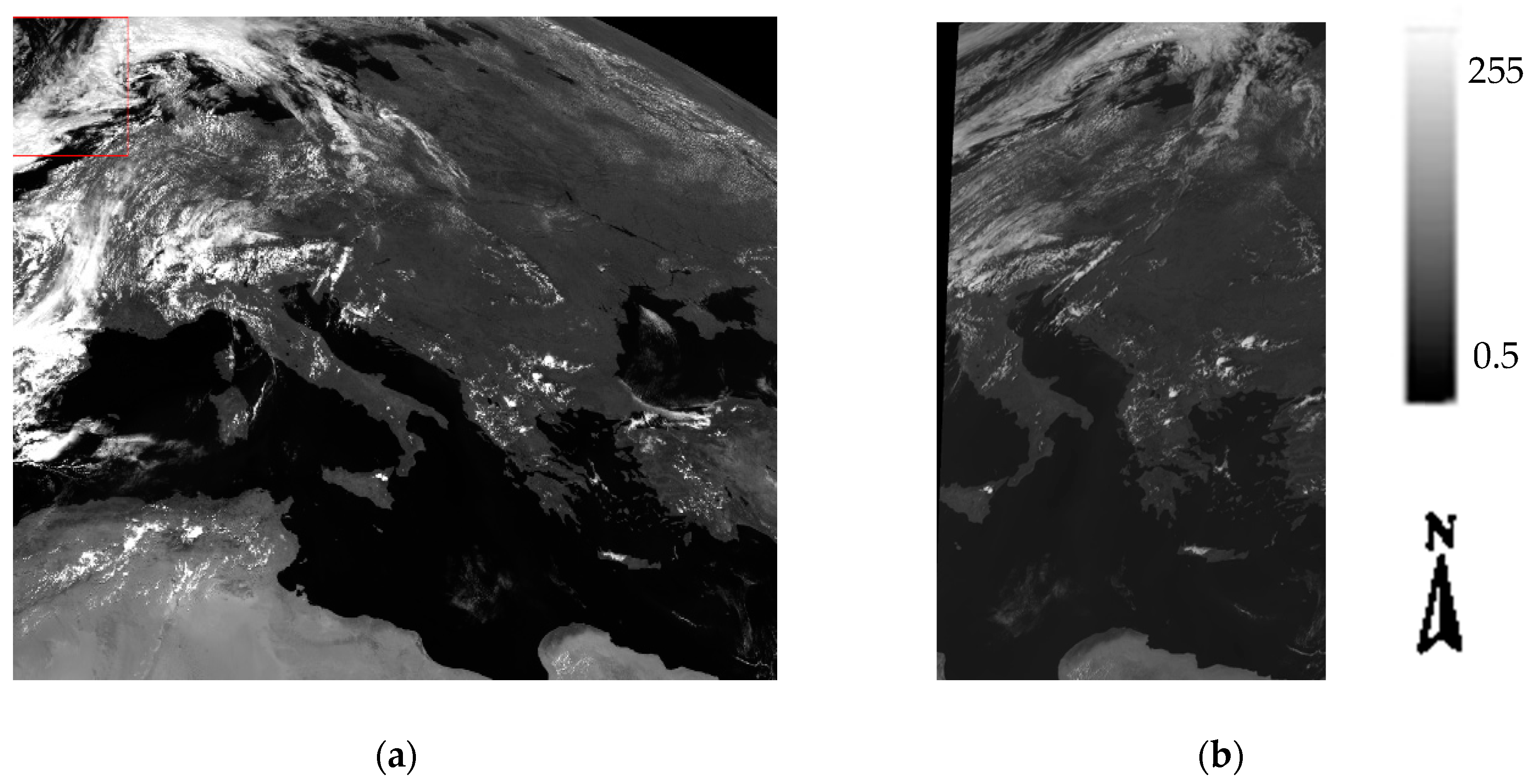
2]. However, it is worth mentioning that before the publication of this research paper, the Meteosat-10 platform has been replaced by Meteosat-9 RSS and located at 9.5° E since 20 March 2018, and afterwards Meteosat-11 has been located at 0° E since 20 February 2018. Therefore, similar research can be implemented using Meteosat-11 instead of Meteosat-10 image data. An overview of the selected stereo image pair in our study and the corresponding study area is shown in
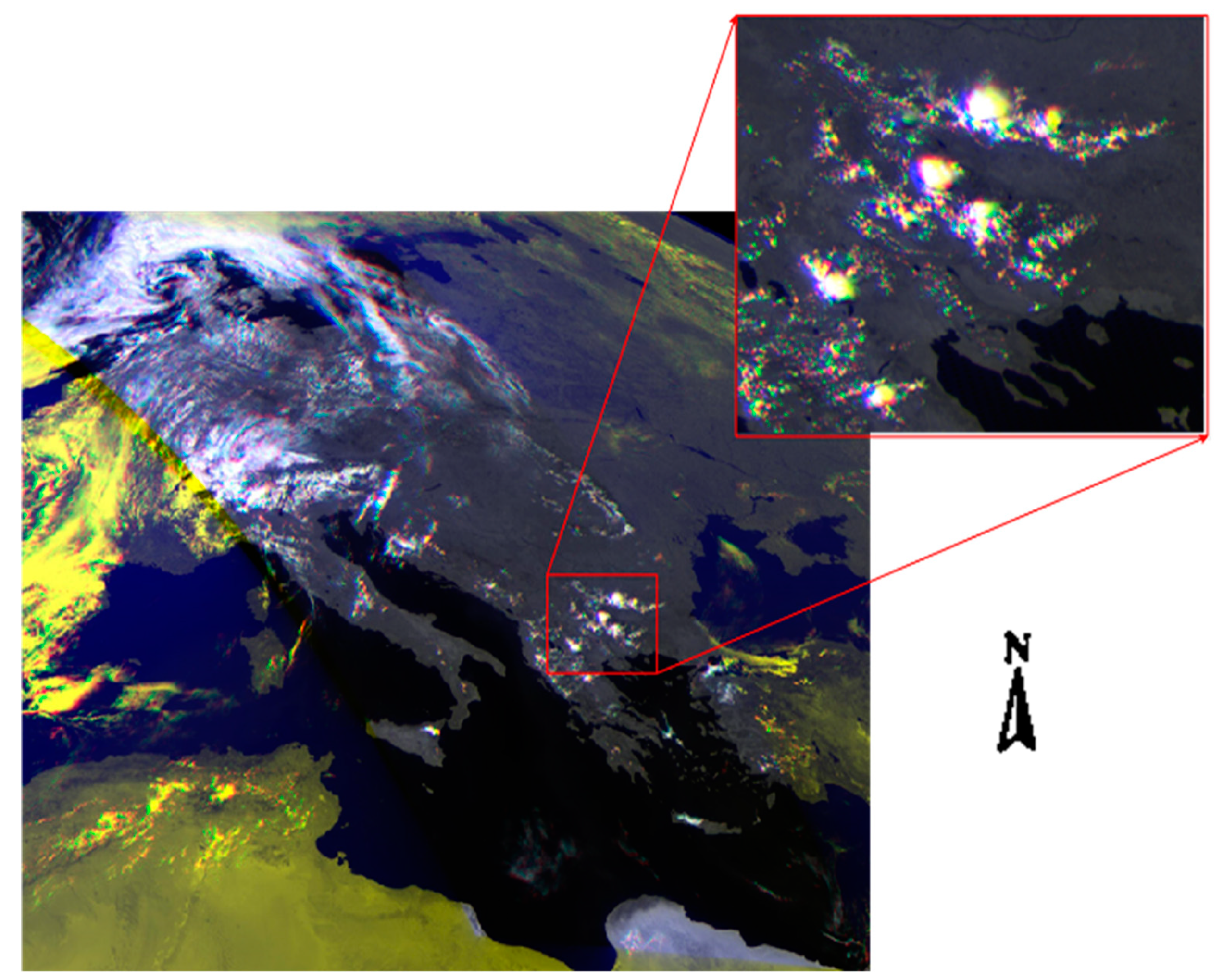
Figure 1.
The introduced image data were downloaded from EUMETSAT data center (
https://www.eumetsat.int/website/home/Data/DataDelivery/EUMETSATDataCentre/index.html), in level 1.5 and in High Rate Image Transfer (HRIT) mode. Level 1.5 image data corresponds to the geo-located and radiometrically pre-processed image data, ready for further processing, e.g., the extraction of meteorological products. Any spacecraft specific effects have been removed, and in particular, linearization, and equalization of the image radiometry has been performed for all SEVIRI channels. The on-board blackbody data has been processed. Both radiometric and geometric quality control information is included.
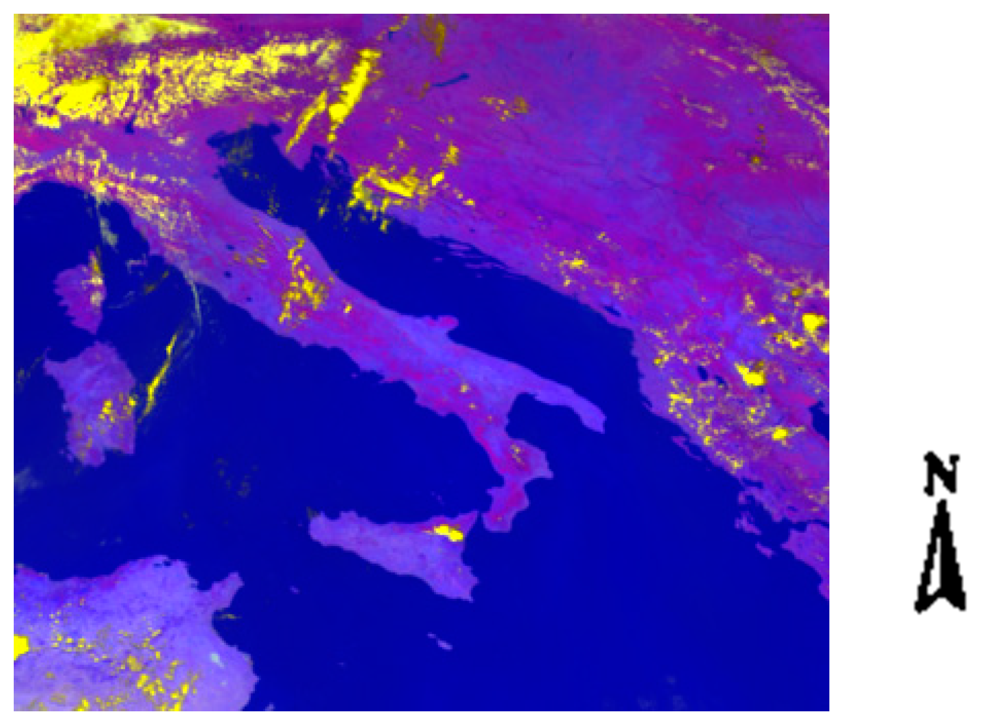
Moreover, in order to provide the possibility of comparing the resulting outputs from the proposed approach with other detection methods, multispectral non-HRV bands of a specific subset in the same region were also used. The color composite of the visible and near infrared spectral bands (VIS: 0.8, VIS: 0.6, IR: 8.7 μm), is shown in
Figure 2.
4. Results
In the following subsections, the step-by-step results for each part of the process are presented.
4.1. Re-Projection into a Reference Image Grid
In order to provide a single reference grid with a similar spatial resolution and projection, the Meteosat-8 (IODC) image was projected on the Meteosat-10 (longitude = 0° W) spatial grid. For this purpose, both linear and IWD resampling methods were investigated. Our experimental results showed that the linear resampling had more interpolation artefacts in comparison to IWD. Due to the fact that a lesser number of artefacts leads to better image matching, an IWD interpolation technique was used in this study as the main resampling approach. Though, IWD resampling required a much longer processing time in comparison to the linear and bilinear resampling methods.
In order to control the location accuracy of the images, after this projection, all coastlines, whereby the height difference is zero, were aligned in both images. Consequently, if an object has a height, its location must be changed in the reference grid, in proportion to its height.
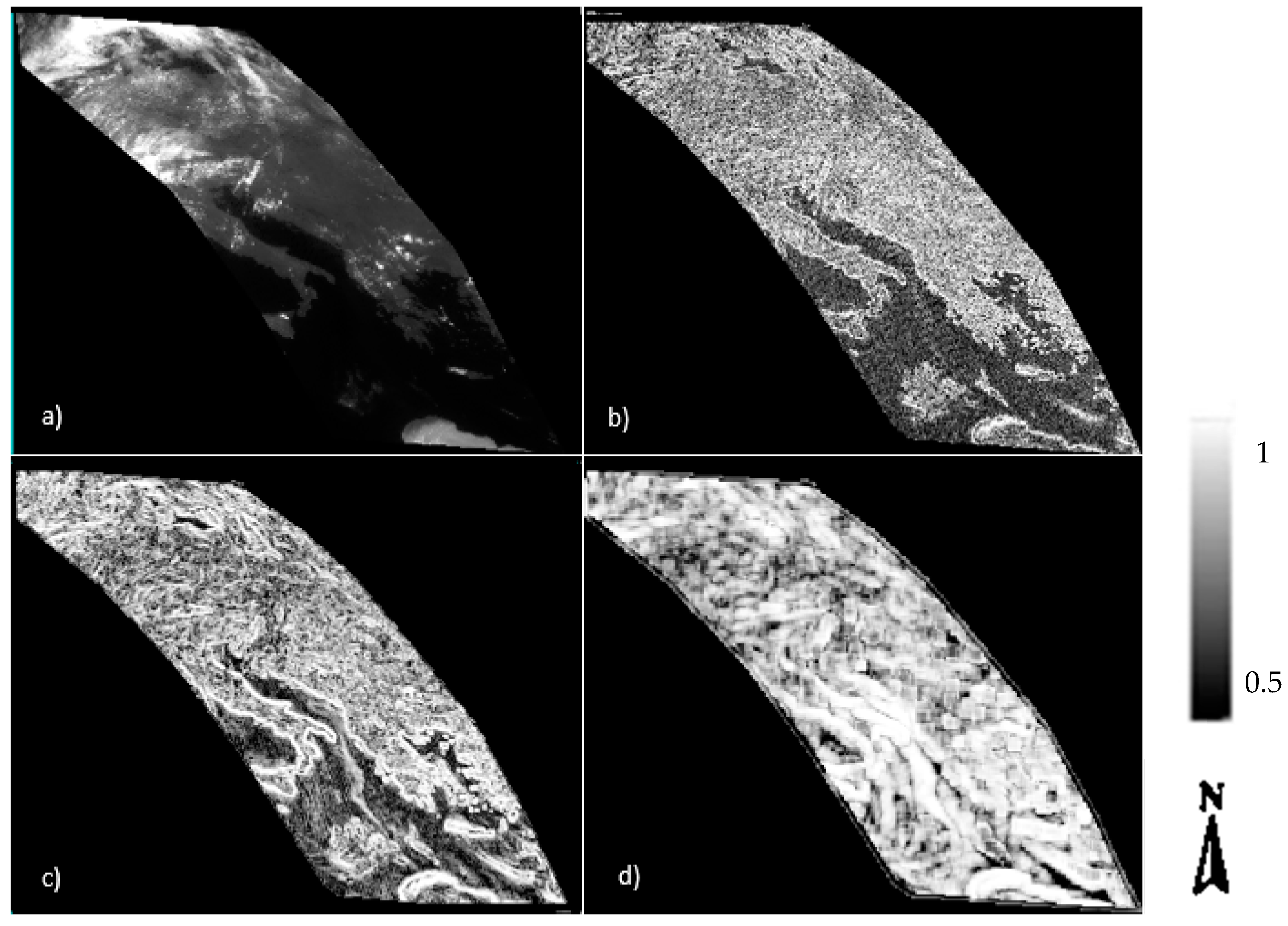
Figure 8a shows the re-projected Meteosat-8 (IODC) image on the Meteosat-10 reference grid.
4.2. Image Matching and Co-Registration Outputs
The main objective of this step was the determination of tie points in between stereo pairs based on an automatic image matching technique. The image matching approach applied in this research is similar to the one used by Zakšek (2013) [
19] and Merrucci (2016) [
28]. As mentioned before, in this study, the image correlation was estimated at different levels of the image pyramid to better determine the tie points. At the upper levels of the pyramid, the spatial resolution varies proportionally to the selected coefficient in that level. In this study (referring to [
21]), coefficient 3 was used. Thus, the value of the image shift and correlation index (CI) was computed for all the pyramid levels, and if the correlation index value at the end of the pyramid (with the least spatial resolution) was less than 0.7, then the calculated shift value was considered as unreliable and zero was used instead (see [
14]).
In this study, due to the good results obtained in [
19,
28], the dimensions of the moving and search windows were selected respectively by 7 × 7 and 13 × 13.
Figure 8b–d shows the correlation index in different levels of the pyramid. The brighter the image pixel in this figure, the higher the correlation index.
As a result of image matching, the amount of shift between image pairs was also generally estimated and tie points were selected based on the highest correlation in between the image pairs. Finally, the resulting output from this step was a file with in which image coordinate pairs like () for the entire tie points are presented. As a result, 2,102,398 tie points were generated automatically between the stereo pairs.
Since the accuracy of height estimation is directly influenced by the image matching results, it is necessary to examine the relative co-registration of the stereo pairs after doing the registration. A visual tool for fast quality control is the application of a color composite in a Red, Green and Blue (RGB) space. The first SEVIRI was chosen as the red and green bands, and SEVIRI-IODC for the blue band.
Figure 9 shows such a color composite. As is clear from this figure, all the coastlines are overlaid on top of each other in all images. It can also be seen in the magnified red polygon that the clouds are more detectable with the existing parallax in the images in comparison to each of the single gray-scale channels.
After tie point generation and ensuring the accuracy of the results, it is possible to form the 3D linear equation (Equation (3)) to estimate the amount of parallax between the image pairs and finally cloud height. Hence, in the following subsection, the results of solving the equations in
Section 3.3.4 (intersection) are given. In addition, some of the mid-level outputs of the cross-correlation analysis in different image pyramid levels are provided as
Supplementary Materials (see Figures S1–S6 in SM-5).
4.3. Parallax Estimation (Intersection)
As it was mentioned in
Section 3.3.4, after the image matching, tie point selection, and coordinate system conversion, the intersection equation (Equation (3)) was solved for the stereo pairs. As a result, two parameters, including the value and minimum intersection distance, were estimated.
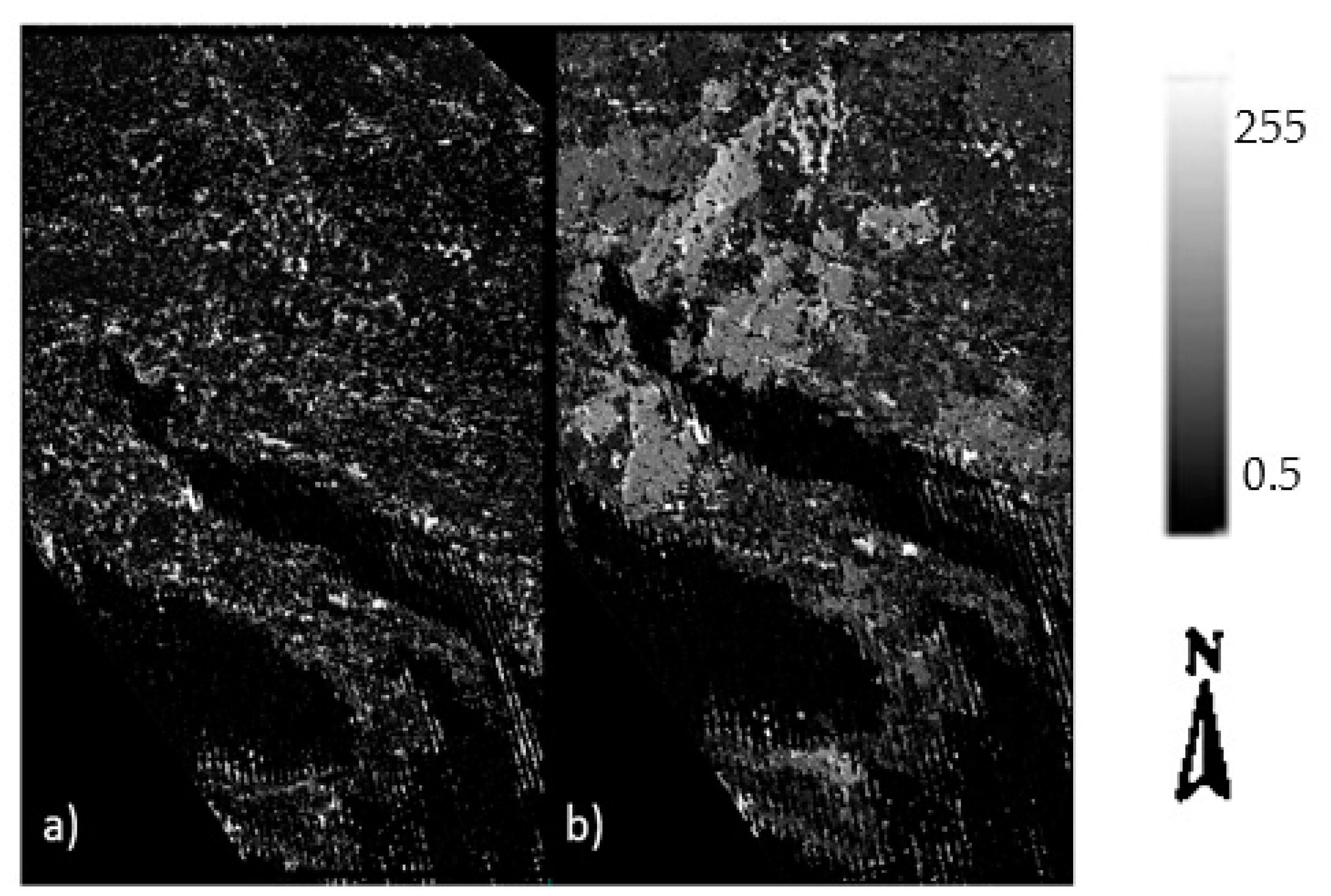
Figure 10 represents both the estimated parallax value and minimum intersection distance in our study area.
The distance between the epipolar lines in the epipolar geometry (
d), i.e., the minimum intersection distance, indicates the accuracy of the height estimation. Given that
d is a measure of intersection uncertainty, it should be as small as possible. The less the distance, the darker the corresponding pixels of
Figure 10a, and the more precise the resulting output.
The parallax results are different in that the higher the parallax value, the higher the probability of having cloudy pixels. Therefore, in
Figure 10b, the brighter the pixels, the higher the parallax in between the stereo pairs [
60].
4.4. Results of the Proposed Detection Method Based on the P-d Feature Space
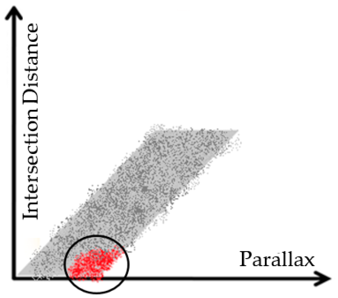
Looking at
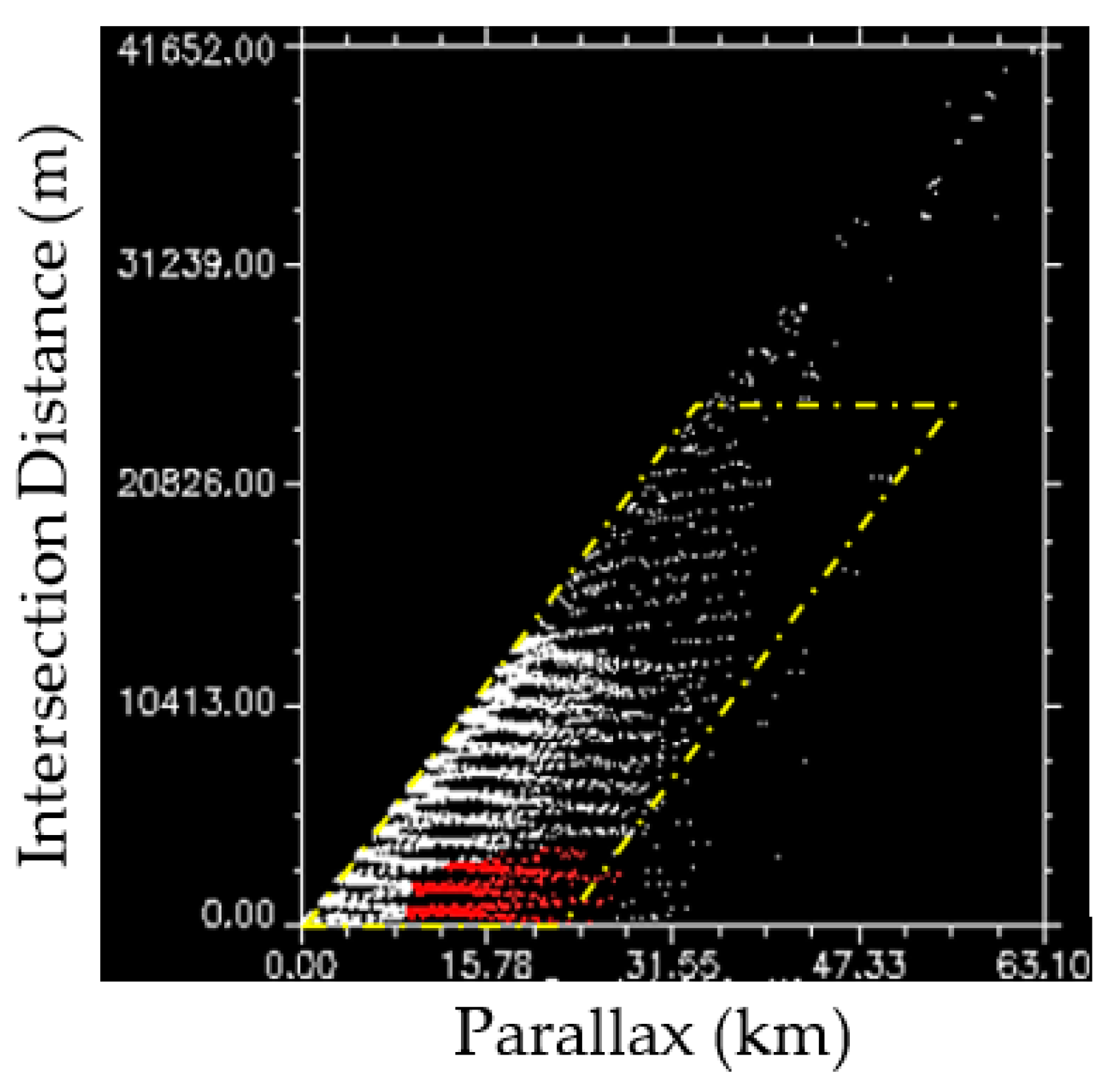
Figure 10b, it is clear that the cloudy pixels were determined quite well based only on their parallax shift. However, in order to more precisely detect the clouds from other pixels in the image, simultaneous use of the minimum intersection distance (d) and parallax (p) in a 2D scatterplot is proposed (
Figure 11). The decision making for being a cloudy pixel is to minimize the former and maximize the latter (see
Figure 6) in the 2D scatterplot. In
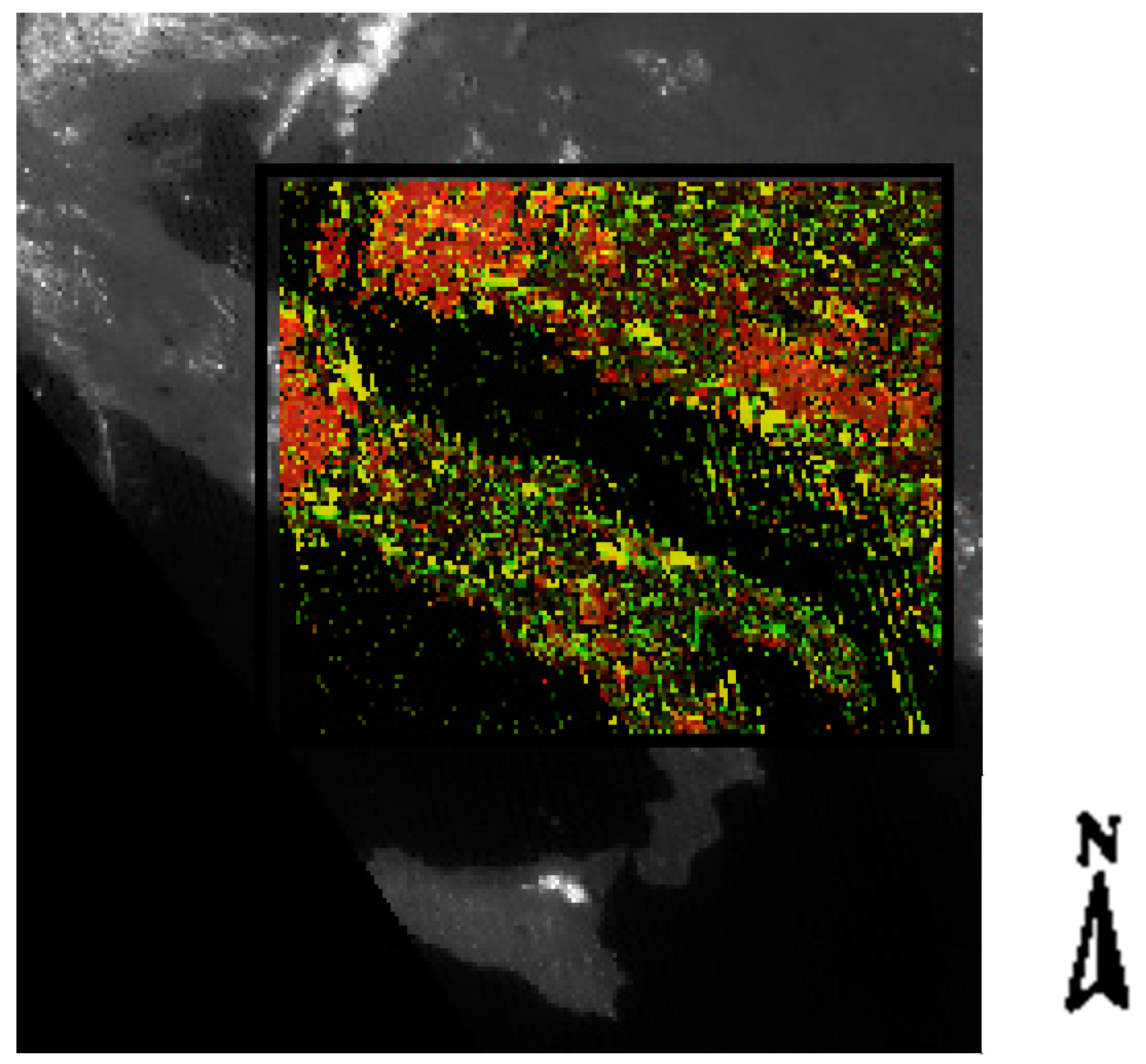
Figure 10, the red selected region, represents the cloudy pixels. The linked image subset with the scatter plot in
Figure 11 is also shown in
Figure 12. However, only one subset of the image is shown in
Figure 12 for the sake of better visualization and comparison. As can be seen in
Figure 12, and by comparing the results with
Figure 9, the red region is completely concentrated on the cloudy pixels. Therefore, as a visual evaluation of the results, it seems that the model and the proposed feature space work perfectly for cloud detection purposes.
Although the visual evaluation of the results seems trustworthy and acceptable, nevertheless, for a better validation, the results of this detection were compared with three well-known target detection techniques in remote sensing, including CEM, MF, and ACE. In the following subsection, the results of this comparison and better validation of the results are presented.
4.5. Comparison with Other Target Detection Methods
In order to evaluate the results of the proposed detection approach, three common target detection techniques, including ACE, CEM, and MF, were implemented on the Meteosat multispectral images. The color composite of the visible and near infrared spectral bands (VIS: 0.8, VIS: 0.6, IR: 8.7 μm) is shown in
Figure 2.
After introducing the multispectral image in
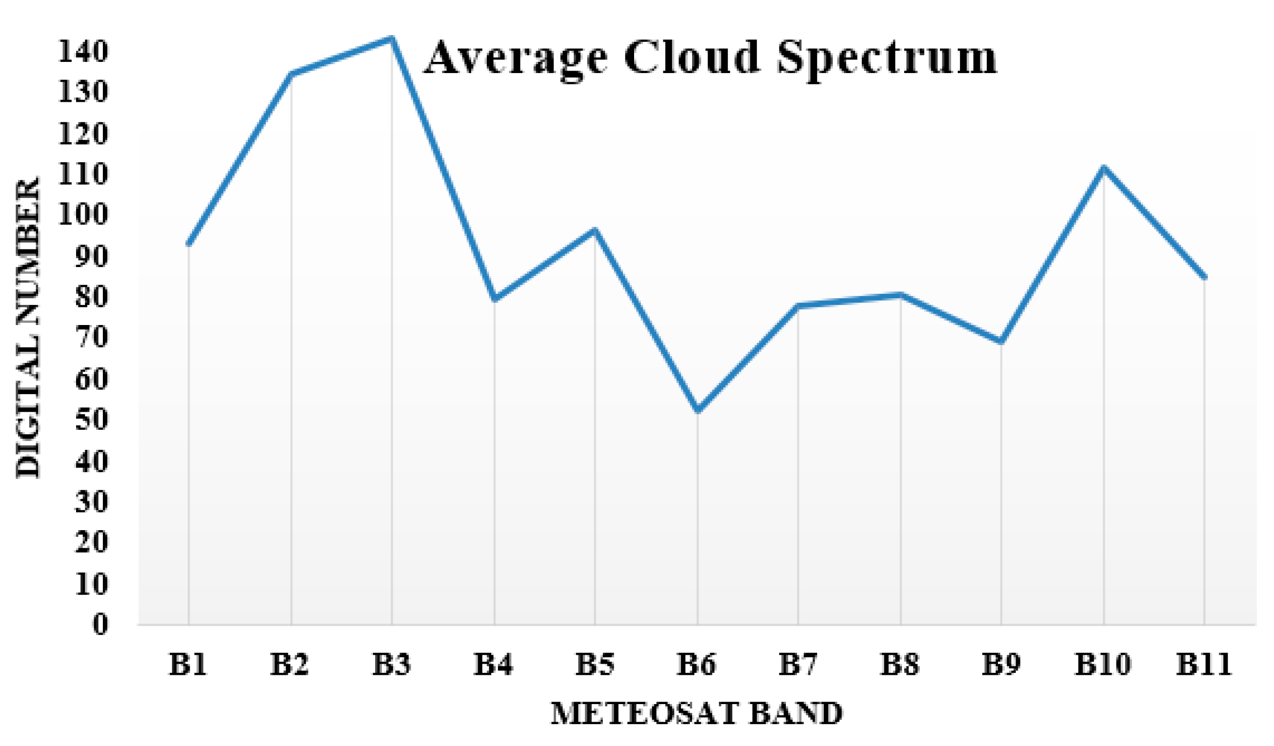
Figure 2 and selecting the ROIs manually (from two specific cloud and no-cloud targets), the three above-mentioned detection algorithms were implemented. For this purpose, the average cloud spectrum based on the selected ROIs in cloudy regions was first produced. The mean cloud signal obtained from the selected cloudy ROIs is shown in
Figure 13. This spectrum is used as training spectra, which will be used as input in the detection models. By the way, it should be mentioned that a minimum noise fraction (MNF) transform [
67] was also implemented on the raw multispectral image to reduce the spectral noise. Afterwards, the set of detection algorithms were performed respectively on the images.
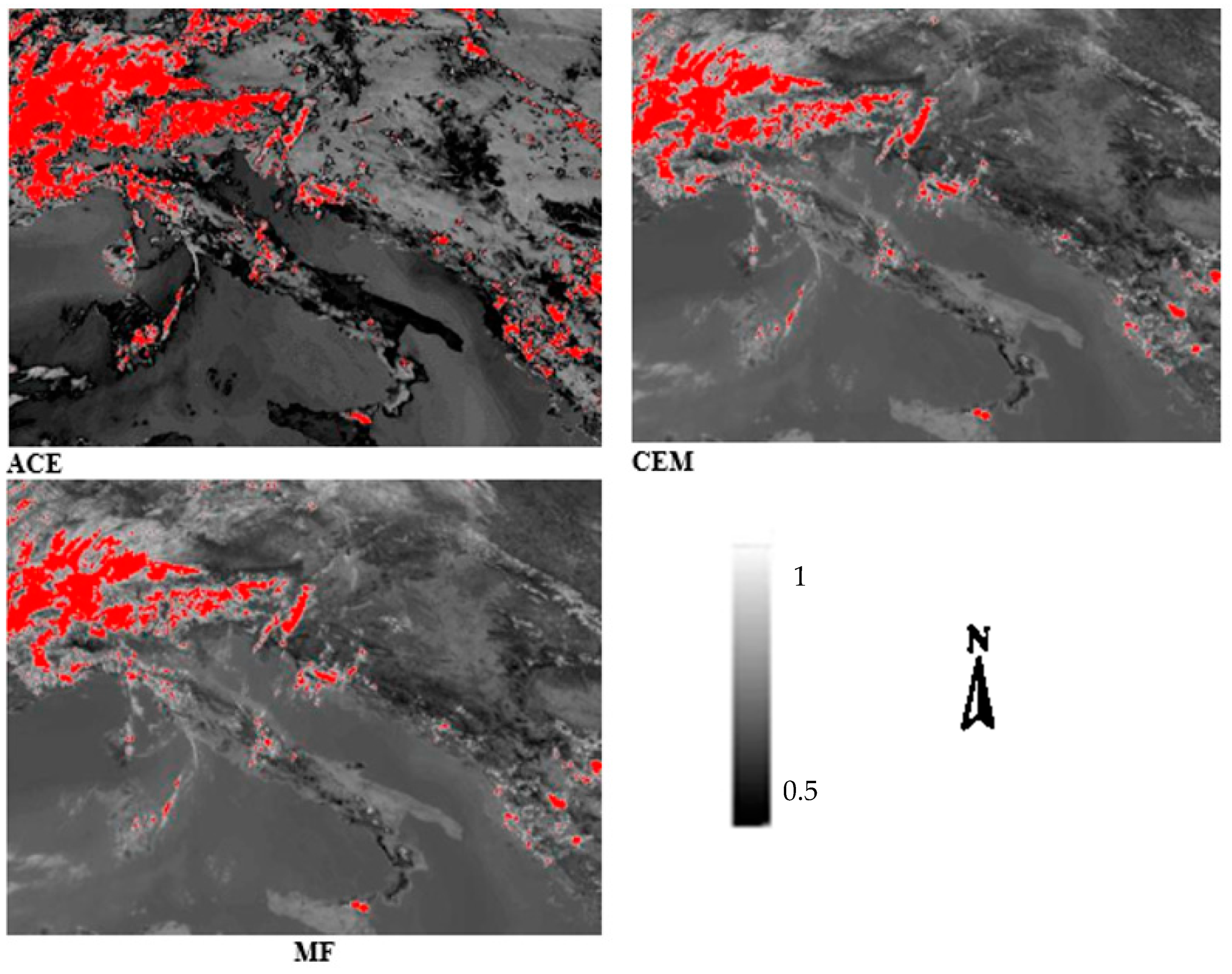
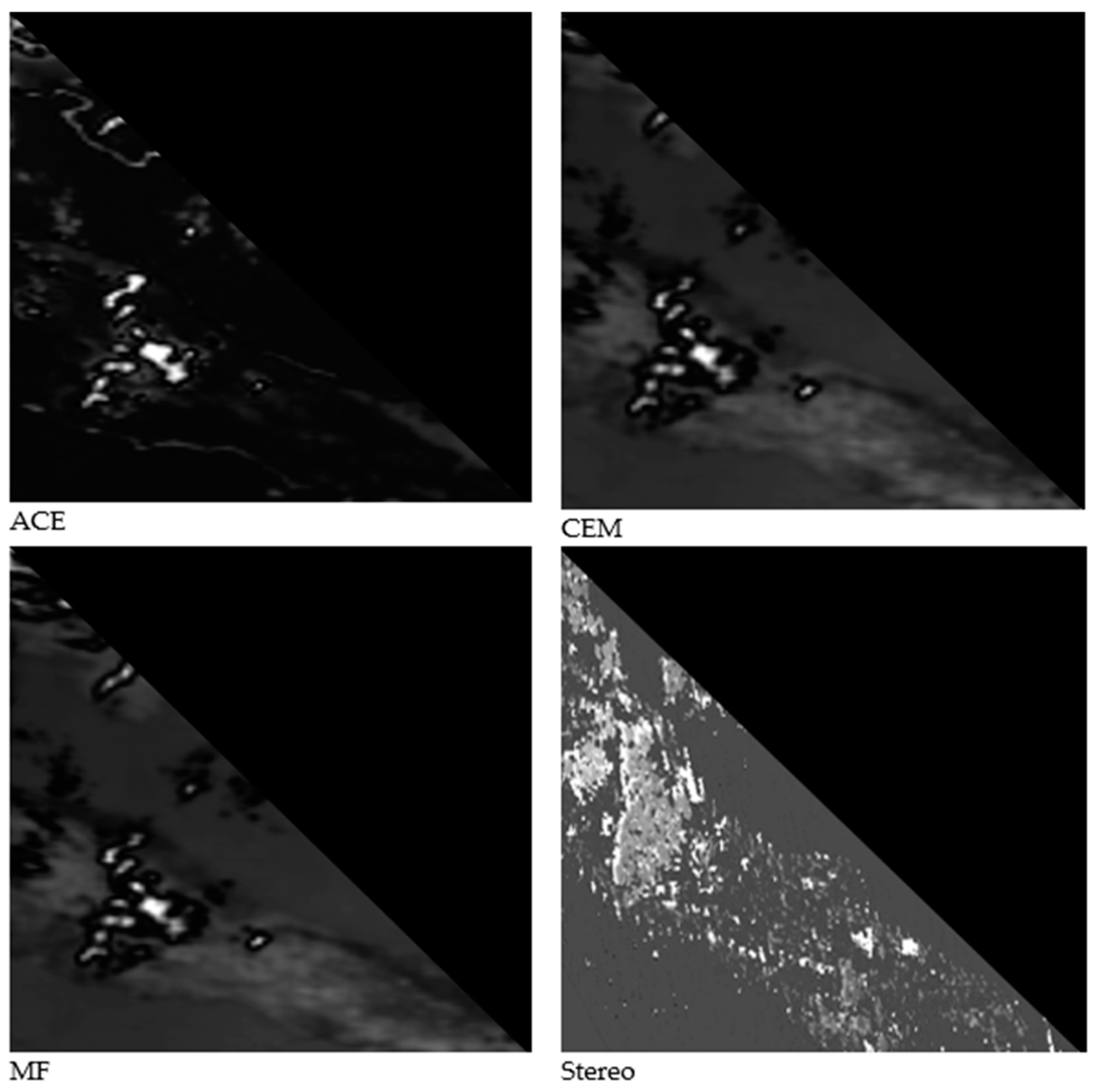
Figure 14 represents the resulting detection outputs from these algorithms in a smaller subset of our study area.
As is clear from
Figure 14, the three mentioned algorithms worked well for the detection of clouds with specific detection probability thresholds of 0.70. The output probability maps and detection results from the MF and CEM methods are quite similar to each other.
In
Figure 14, the brighter the pixels, the higher the probability of detection, which is normalized here to 255 because of the better visualization. The detection results are only visually comparable in
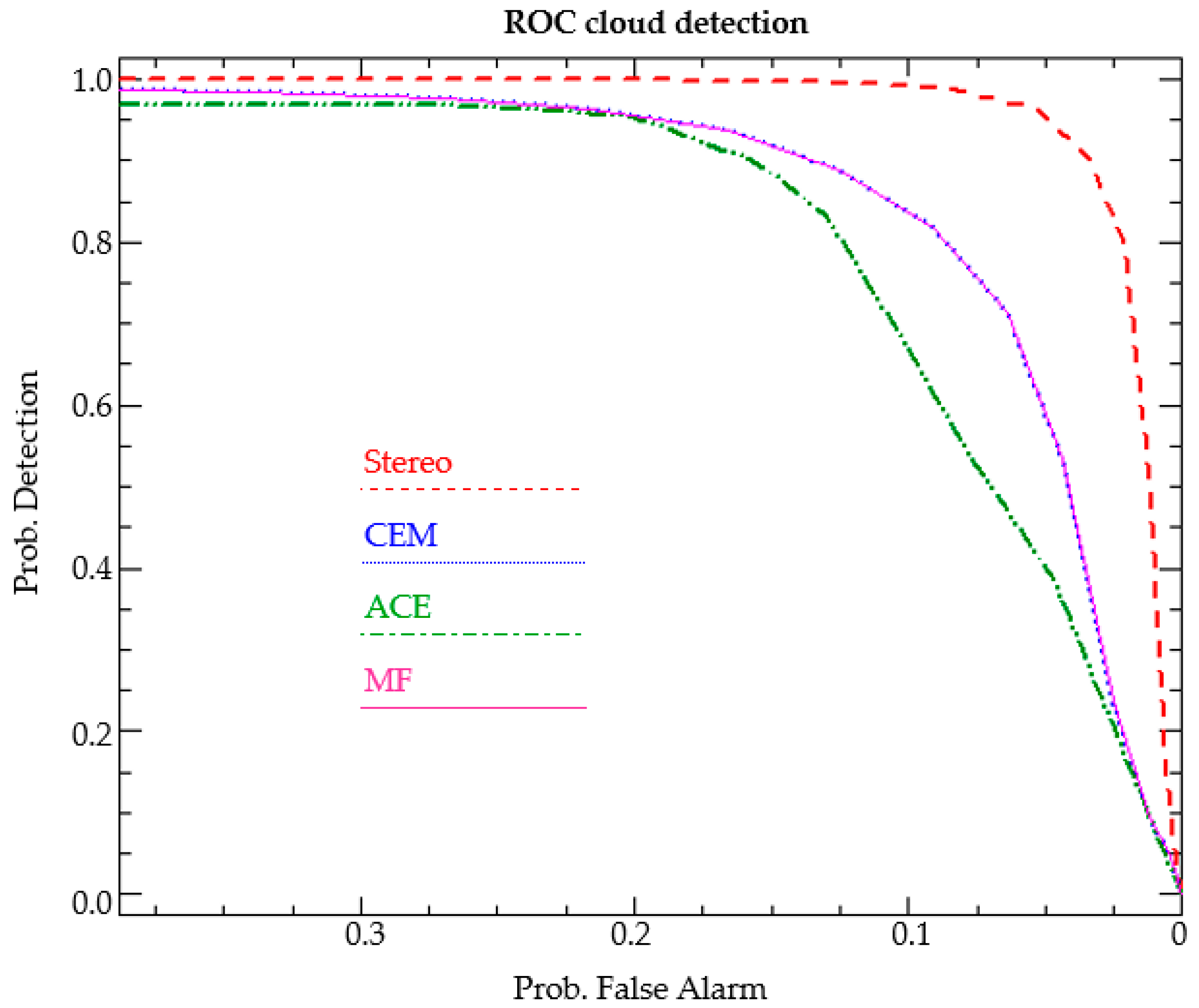
Figure 14. Hence, for the sake of a better performance comparison, the conventional receiver operating characteristic (ROC) curve [
47] was used (see
Figure 15).
After having a precise look at the curves shown in
Figure 15, it is clear that the detection performance was similar in both the CEM and MF methods while the ACE method had a weaker performance. This comparison suggests a better detection power for the proposed method. As is clear from
Figure 14, some low-density clouds were not clearly detected using the common target detection techniques.
In addition, in order to provide a quantitative comparison of the results, an area under the curve (AUC) criteria was also calculated for the methods. AUC stands for the area under the ROC curve. This criterion measures the entire two-dimensional area underneath the entire ROC curve (think integral calculus) from (0, 0) to (1, 1). The AUC value lies between 0.5 to 1, where 0.5 denotes a bad classifier and 1 denotes an excellent classifier [
47].
Table 1 shows the calculated AUC values for the different methods. The interesting result is that both the MF and CEM methods had similar AUC values. Although, the ACE method detected the clouds not very badly, but it was the weakest method in this study for the detection of clouds. Finally, as is clear from
Table 1, the best detection performance was for the stereo-based approach, with AUC = 0.93.
A general look at the current results suggests that although the common spectral-based target detection techniques have recognized cloudy pixels well in most areas, these techniques did not work very well in very mixed pixels and for small or quite transparent clouds. These kinds of clouds were better detected in the proposed stereo-based approach. Nevertheless,
Figure 12 shows more noisy outputs in the proposed method. Although, because of the application of the HRV band in the proposed approach, the corresponding detection results originally have a better spatial resolution in comparison to the other detection methods.
In addition, according to the fact that the ROC analysis did not take into account local variability within the results, the so-called local Moran’s I index [
68] as a local spatial statistic was also applied. This index is available in the ENVI toolboxes. The local Moran’s I index identifies pixel clustering. Positive values indicate a cluster of similar values while negative values imply no clustering (that is, high variability between neighboring pixels). ENVI uses the Anselin method [
68] for the Moran’s I index by computing a row-standardized spatial weights matrix and standardized variables (see
https://www.harrisgeospatial.com/docs/LocalSpatialStatistics.html for more details).
Figure 16 presents the result of this analysis on a small image subset from all detection methods.
From
Figure 16, which shows only a small part of the image, it seems that the entire detection methods showed less variability near the clouds. However, it seems that near the borders of clouds, there are more variabilities for both MF and CEM, and less variabilities respectively for ACE and stereo.
4.6. Other Characteristics of the P–d Space
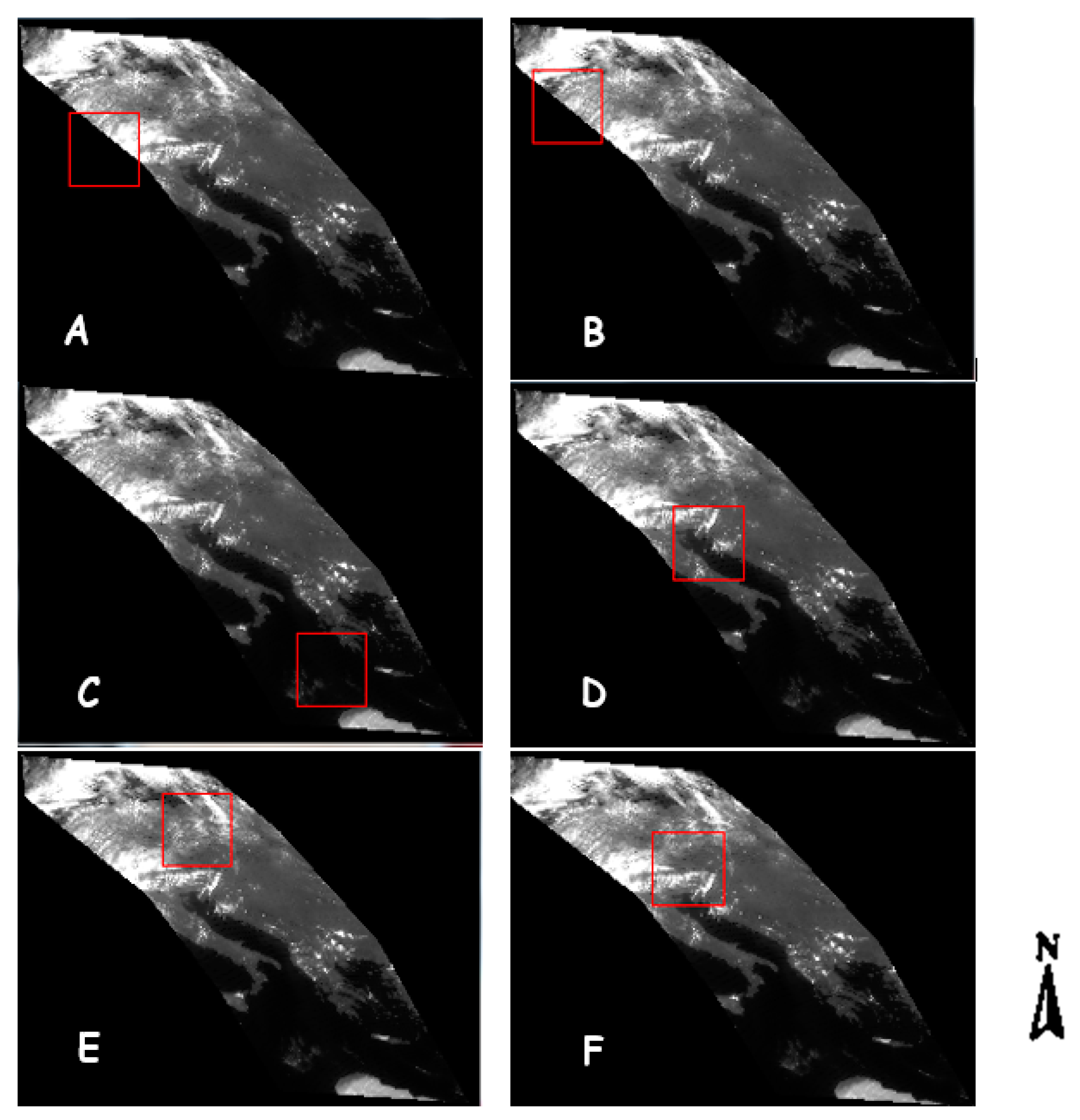
Our experience with different image subsets showed that the characteristics of the represented parallelogram in the 2D feature space is changing in different regions based on the amount of cloud cover and probably the cloud type. For better clarification of the changing characteristics of the resulting parallelogram space, we provide the P–d scatter plots in different subsets of the entire image. These subsets and their corresponding P–d scatter plot are respectively shown in
Figure 17 and
Figure 18.
In
Figure 17, we tried to select and analyze the image subsets in regions with different amounts of cloud cover.
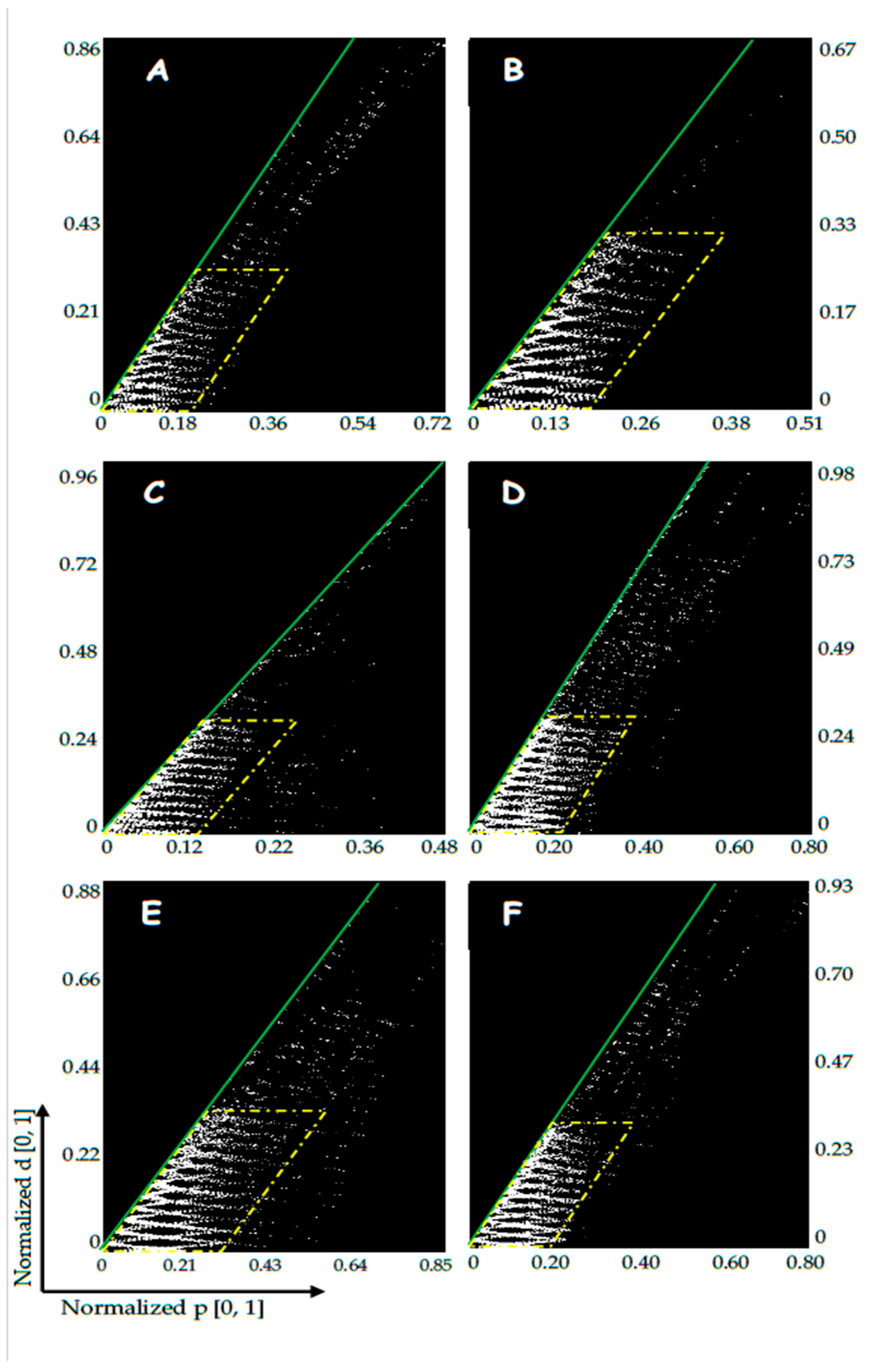
Afterwards, for each region, a suitable parallelogram was fitted to the pixel points in the P–d feature space (yellow polygons in
Figure 18). The red dashed line is drawn from the coordinate system origin point to the other end of the coordinate system. The green line is tangent to the points and shows the slope of the parallelogram in this space.
A visual comparison of the graphs and images in
Figure 17 and
Figure 18 shows that the lower the amount of clouds in a region, the smaller the slope of the green line in
Figure 18. For example, in
Figure 17C, there is no cloud in the subset and as a result the green line has a higher slope angle to the x-axis.
Hence, the slope angle of the green lines can be introduced as a representative value, which shows the amount of cloud clover. In order to provide a better numerical comparison, the slope angle of the green line was calculated for all the graphs in
Figure 18.
The results of the slope angle calculations, which are shown in
Table 2, seem very interesting. As is clear, the lower the amount of cloud cover, the bigger the estimated slope angle. For example, in image subset C, the least amount of cloud cover exists, and it has the biggest slope angle in comparison to other subsets. The mentioned result was already expected, since the bigger slope angle corresponds to a smaller parallax value and bigger intersection distance.
A precise look at the normalized values of both the parallax and intersection distance in
Figure 18 shows that these values are changing for each image subset. As it was also expected, the lower the amount of clouds in an image subset, the lower the maximum value of the parallax (see
Figure 17C and
Figure 18C). From the analysis on the different image subsets and their corresponding P–d space, we came to the conclusion that cloudy pixels have a parallax value bigger than P = 0.1. However, the intersection distance range does not generally change very much among the various image subsets. Nevertheless, the same threshold value (d = 0.1) for this parameter seems to also be applicable for the detection of cloudy pixels.
Nevertheless, it is worth mentioning that these values cannot be generalized to all other places, atmospheric conditions, and/or images or scenes. Hence, for a general threshold value suggestion, more research on different image scenes, various amounts of cloud cover, other geographical locations, daytime and seasons, etc. are required.
Another interesting behavior in this graph is the several semi-parabolic shapes, which are located on top of each other and their central point is tangential to the green line. These parabolas show the mathematical relation between the P and d, shown in Equation (5):
where
P1 and
P2 are respectively the parallax values for the first (left) and second (right) images in the stereo pair.
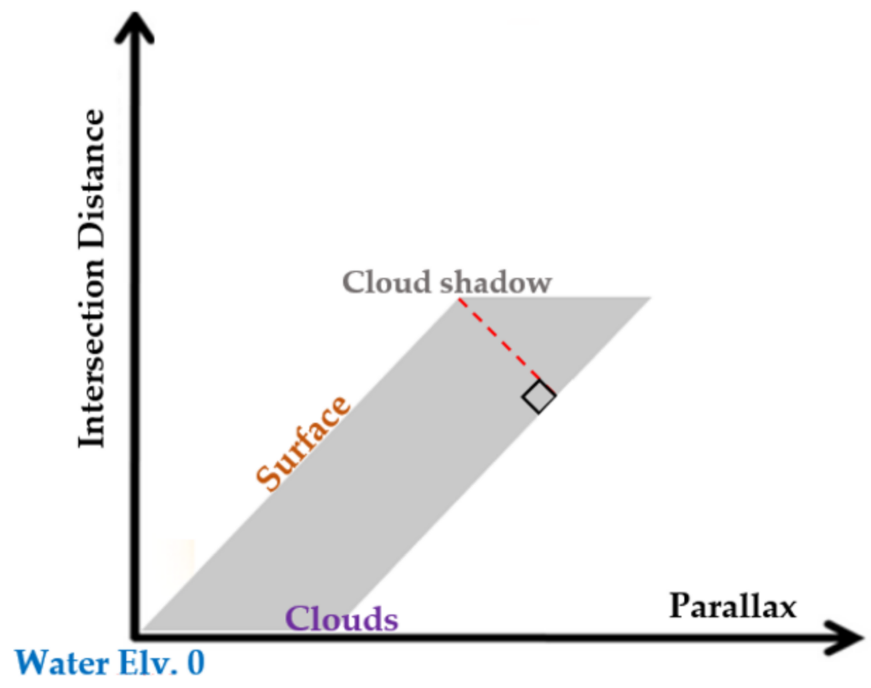
Our analysis on the graphs and image pixels also showed that the left side of the parallelogram that is tangent to the green line holds the elevation information of the ground objects. As can be seen, the base of the yellow parallelogram overlays on the x-axis and its slope shows the slope of the green line. Hence, this information shall be later used as a criteria/index to present the amount of cloud cover in an image. This information is summarized in
Figure 19.
It is worth mentioning that we also checked the data points above the yellow parallelogram and the conclusion was that they mostly contained not very much information about clouds because the accuracy of estimation in those points are very low (d has big values).
In the next section, a brief discussion on the above-mentioned results is given.
5. Discussion
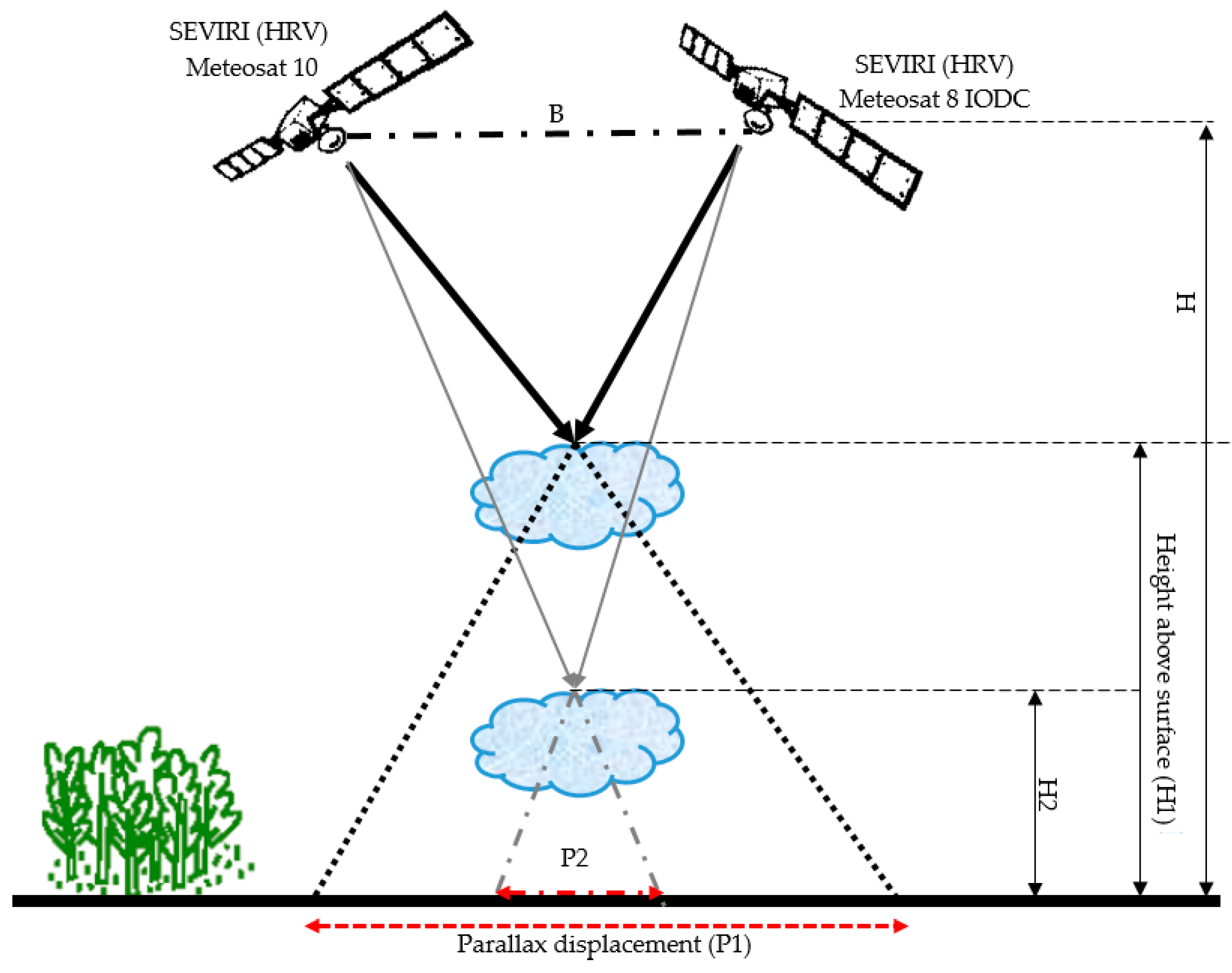
The image data used for this stereo analysis included the HRV bands from two identical SEVIRI sensors, which were on board two platforms in 0° W and 41.5° E geographical longitudes. We did not use the Rapid Scan Services (RSS) mode, because in this mode, the acquisition of the first sensor takes place at 9.5°E and as a result the spatial baseline, i.e., the distance between the two stereo pairs (parameter B in
Figure 4), will decrease. As a consequence, the height estimation accuracy of the stereo model will also decrease. It is, however, worth mentioning that the lower spatial baseline may improve the image matching results, but because of the low time difference between the HRV pairs (i.e., 5 s), the matching was improved in this study. This 5 second time difference is because images from the second generation of Meteosat are taken every 15 minutes using a line by line scan basis. Therefore, we have a specific acquisition time for each image line and a time range for each picture. For example, in our data the start and end time of the image acquisition were 11:45:09–11:57:39 and 11:45:10–11:57:44 respectively for the Meteosat-10 and Meteosat-8 (IODC), which confirms the maximum 5 seconds time difference between the stereo pairs.
Since the accuracy of the height estimation depends on the so-called baseline-to-height ratio (B/H) [
69], the higher the B/H value, the more precise the height estimation results. It should also be noted that this statement is true for the coarse resolution data—with the HRV bands (~ 1 km) that is still our case—but this statement might not be valid for higher resolution images because of the problem of image matching. As a consequence, it is clear that the longer baseline (in coarse resolution data like our data) results in a better accuracy.
From a general view of our research, there is a list of benefits to be mentioned: (1) The lower time difference between the stereo pairs (see
Figure 1a,b); (2) the higher spatial baseline (higher B/H value, consequently higher height/parallax accuracy); (3) better spatial resolution because of the application of HRV bands. Thereupon, the differences in between images related to the cloud movements and other temporal changes is the smallest; and (4) both sensors have a similar radiometric resolution (10 bit), which makes the texture analysis much easier.
In this research, both image pairs were acquired by similar sensors with a comparable spectral/spatial response function. Therefore, higher quality of the tie point selection is expected in comparison to that of [
28]. However, there are still some differences, like the solar illumination condition and viewing geometry, which makes one specific object in the overlapping region of image pairs appear differently in each. Thereupon, finding highly correlated tie points was more difficult. Hence, a Wallis filter was applied on the raw images to remove the effect of different illuminations. Nevertheless, according to the given definition of clouds in
Section 1, there might still be difficulties in performing the image matching, especially when transparent clouds are located on top of very heterogeneous regions. This needs to be investigated with further research.
On the other hand, image texture might be a problem only if the spatial resolution of the input data is very fine or too coarse. Considering SEVIRI, meteorological clouds usually have enough structure (texture) in the HRV channel [
28] for image matching.
In addition, one other main drawback of this method is also that the accuracy of the results is dependent on the positional accuracy of the input images. It is not particularly important for the absolute geolocation to be accurate, but the co-registration between the images from both satellites must fit perfectly. For this reason, it makes sense to check the co-registration accuracy during pre-processing when all datasets are transposed to the same coordinate system. This can be done automatically by adjusting the co-registration along coastlines.
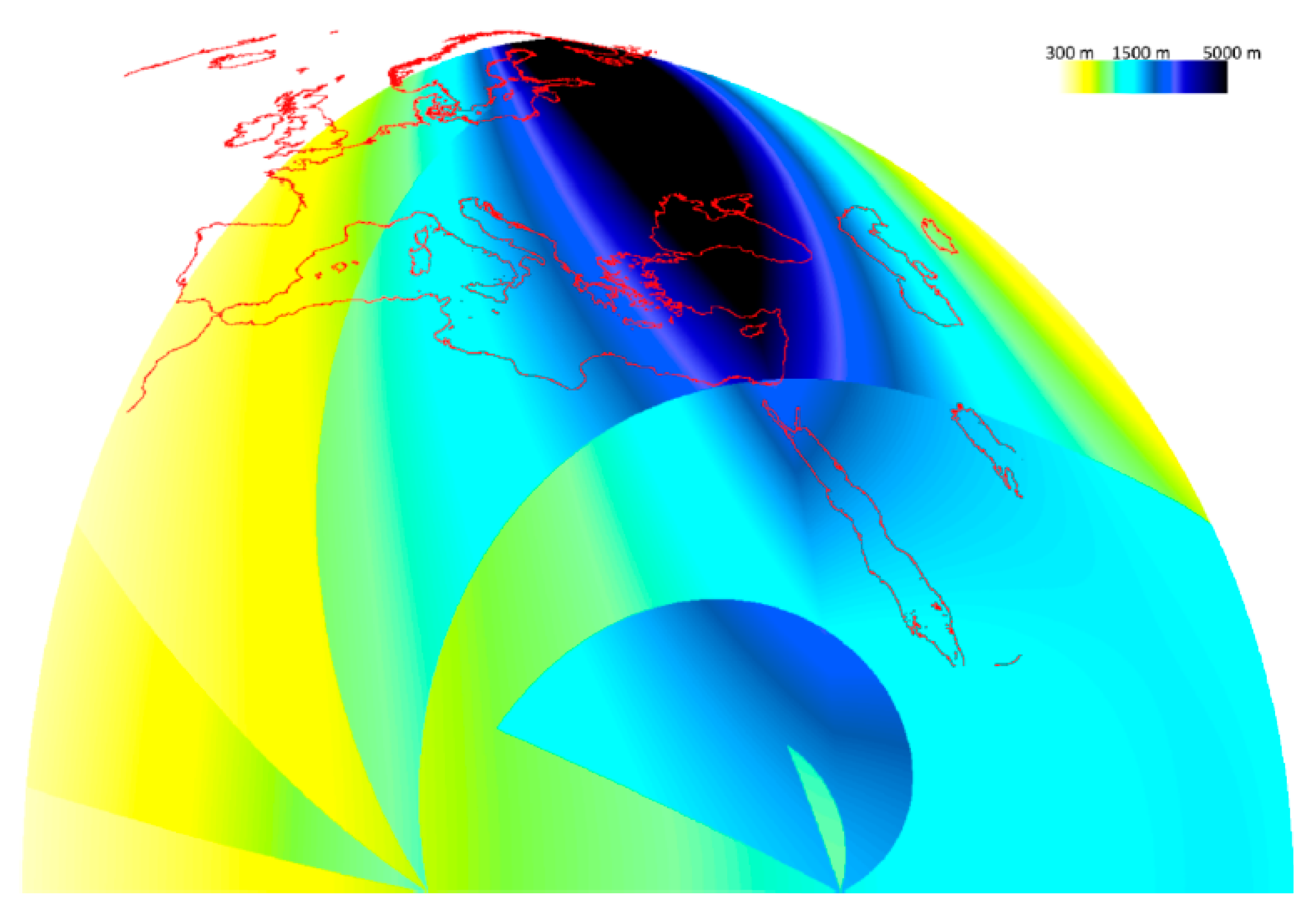
One potential source of inaccuracy in the results is that the spatial resolution of the Meteosat pixels reduces near their margin. It means the pixel size become bigger. Thus, it is expected that the spatial resolution of the IODC image in the overlapping part of the stereo pair is worse than 1 km (around 2–3 km), which will affect the accuracy of correlation in between both pairs, tie point determination, and finally, the height estimation accuracy. Nevertheless, in a stereo study by Merrucci et al. (2016) [
28], an analysis on the accuracy of the results was performed. This analysis was performed assuming the spatial resolution of both stereo pairs was similar. In our study, we are much closer to this assumption in comparison to [
28], because of the application of HRV bands from the similar sensor in both pairs. However, this investigation showed that the accuracy of estimation is between 150 and 2500 m and the minimum detectable cloud height is two-fold, i.e., varies in the range 300–5000 m. To see more details about how these investigations were performed, see [
28], and
Figure 20, which shows the resulting accuracy estimation from [
28].
The other limitation to be mentioned is the re-gridding of the images and implementation of the the image matching analysis before their complete georeferencing. This may result in resampling artefacts and location inaccuracies, and consequently, automatic matching with a lower accuracy. Another option would have been to resolve the internal and external geometry of each image before parallax calculations. The first reason to do the gridding instead of geocoding is that we would like to test this method later for improving the down-welling solar irradiance (this is currently under study by the authors). In this case, the Meteosat-10 image will stay in its original grid without any radiometric changes, which is important for estimating down-welling solar irradiance. Therefore, we would like to keep the original grid of Meteosat-10 untouched, without any resampling. On the other hand, using the gridding method is a faster approach. Nevertheless, in order to overcome the above-mentioned limitations, first we used the IWD resampling with the least amount of resampling artefacts while gridding. On the other hand, to check the locational accuracy of the images, we aligned the images with the coastlines. This aligning method was previously used in [
28] and was also successful.
From the numerous tests carried out in this study, it was found that image processing software, such as ENVI (Environment for Visualizing Images), PCI-Geomatica, ERDAS (Earth Resources Data Analysis Systems) Imagine, and LPS (Leica Photogrammetry Suit), were not able to estimate the correlation between the Meteosat image pairs and their tie points. Moreover, previous research in [
28] also showed that even with the application of several scale and direction constraints, general categories of automatic image matching methods (including region-based and feature-based [
70,
71,
72,
73]) cannot provide sufficient numbers of highly correlated tie points in between Meteosat images. Therefore, in this study, we used a similar method to the one proposed by Zakšek, et al. (2013) in [
19,
28]. However, as mentioned before, the results of this image matching depends on the size of the search area and the moving window. For example, a large-sized window cannot detect smaller objects, but it can easily detect and extract larger objects and vice versa. Therefore, to optimize the matching results, the best approach was to try local-based image matching and correlation estimation in different levels of image pyramids.
After the image matching, tie point selection, and coordinate system conversion, the intersection equation (Equation (1)) was solved for the stereo pairs. As a result, two parameters, including the parallax value and minimum intersection distance, were estimated. Afterwards, in order to more precisely detect the clouds from other pixels in the image, simultaneous use of the minimum intersection distance (d) and parallax (p) in a 2D scatterplot was proposed.
The decision making for being a cloudy pixel was to minimize the former and maximize the latter (see
Figure 7) in the 2D scatterplot. Comparison of the resulted ROC curve of the proposed detection approach with that of other common detection methods showed that the proposed approach had better results. However, it is worth mentioning that this comparison depends on the selection of two important threshold values: First, the selected threshold for common detection methods (which was in this study the probability value of 0.7); and second, the selected threshold/boundary for classifying cloudy pixels in the proposed 2D scatterplot P–d (equal to 0.1 in the normalized space). Nevertheless, it is worth mentioning that these values cannot be generalized to all other places, atmospheric conditions, and/or images or scenes. Hence, for a general threshold value suggestion, more research on different image scenes, various amounts of cloud cover, other geographical locations, daytime and seasons, etc. is required. Moreover, the detection results of the common methods also depend on the precision of the training ROI set. In addition, a local variability analysis of the results showed that variability near the cloudy pixels is less for the stereo, ACE, CEM, and MF methods.
In the proposed parallelogram space, various tests based on different image subsets were performed. These analyses showed that the parallelogram includes some information about clouds. However, the definition of specified indices and better characterization of this space requires more experimental research, which is currently under more study and investigation by the authors, to ensure the reproducibility of the results.
Generally speaking, the applied stereo approach has been under development for years, simultaneously with the development of new constellations of meteorological geostationary satellites. Therefore, we expect a continuous growing exploitation of this technique in the remote sensing society and specifically weather satellite research.

 ,
, 


