Article

How Well Do Deep Learning-Based Methods for Land Cover Classification and Object Detection Perform on High Resolution Remote Sensing Imagery?

1
School of Computing, Mathematics and Digital Technology, Manchester Metropolitan University, Manchester M1 5GD, UK
2
School of Medicine, Tongji University, Shanghai 200092, China
3
Department of Computer Science, Loughborough University, Loughborough LE11 3TU, UK
4
State Key Laboratory of Remote Sensing Science, Aerospace Information Research Institute, Chinese Academy of Sciences, Beijing 100101, China
*
Author to whom correspondence should be addressed.
Remote Sens. 2020, 12(3), 417; https://doi.org/10.3390/rs12030417
Submission received: 27 November 2019 / Revised: 15 January 2020 / Accepted: 17 January 2020 / Published: 28 January 2020

Abstract

:
Land cover information plays an important role in mapping ecological and environmental changes in Earth’s diverse landscapes for ecosystem monitoring. Remote sensing data have been widely used for the study of land cover, enabling efficient mapping of changes of the Earth surface from Space. Although the availability of high-resolution remote sensing imagery increases significantly every year, traditional land cover analysis approaches based on pixel and object levels are not optimal. Recent advancement in deep learning has achieved remarkable success on image recognition field and has shown potential in high spatial resolution remote sensing applications, including classification and object detection. In this paper, a comprehensive review on land cover classification and object detection approaches using high resolution imagery is provided. Through two case studies, we demonstrated the applications of the state-of-the-art deep learning models to high spatial resolution remote sensing data for land cover classification and object detection and evaluated their performances against traditional approaches. For a land cover classification task, the deep-learning-based methods provide an end-to-end solution by using both spatial and spectral information. They have shown better performance than the traditional pixel-based method, especially for the categories of different vegetation. For an objective detection task, the deep-learning-based object detection method achieved more than 98% accuracy in a large area; its high accuracy and efficiency could relieve the burden of the traditional, labour-intensive method. However, considering the diversity of remote sensing data, more training datasets are required in order to improve the generalisation and the robustness of deep learning-based models.

Graphical Abstract

1. Introduction

The term “land cover” refers to the man-made and natural characteristics of the Earth’s surface, such as water, soil, natural vegetation, crops, and human infrastructure [1]. The land cover and its changes at both regional and global levels can affect our health, environment, etc. Of those, some have been identified as fundamental variables for describing and studying Earth’s ecosystems, such as food production, land management and planning, disaster monitoring, climate change, and carbon circulation [2,3]. Remote sensing data from satellites, aircraft, or Unmanned aerial vehicles (UAVs) have been widely used for land cover to map and monitor the changes of the Earth’s diverse landscapes from Space. A variety of land cover classification and objective detection methods on remote sensed data with high spatial resolutions have been proposed. Broadly, they can be classified into two categories: pixel-based and object-based approaches.
In the pixel-based approach, a pixel in remote sensing data is considered as an independent unit and analysed by its spectral characteristics, geographical location, and time series changes. Each pixel corresponds to a region designated by spatial coordinates, and the information at its geographic coordinates—such as climate, the value time series changes, and even data from other devices—can be used for increasing the discrimination of different categories to facilitate its classification. The pixel-based method has long been the major approach for the classification of remote sensing imagery [4]. Various pixel-based classification methods were proposed based on statistical distance measures [5], including classification and regression tree (CART) [6,7,8], support vector machine (SVM) [9,10,11], and random forest (RF) [12,13]. However, the pixel-based classification method has two major limitations: the first one is the problem of mixed pixels in which the features from multiple classes are presented in a single pixel [14]. It usually occurs in the classification of low and medium resolution images. The mixed pixel problems can be solved through increasing spatial resolution. The second fundamental limitation is that the spatial context from surrounding pixels is not used in classification. Especially when dealing with a high resolution image, the differences in texture features within an object area can result in the differences between pixels in that area, thereby reducing the accuracy of the pixel-based classification. That is called the “salt and pepper” effect [15].
To address these issues, the object-based method was proposed for both high-resolution image classification and object detection tasks using both spectral and spatial information. For a classification task, conventionally, in the object-based methods, similar pixels are firstly aggregated into an object via segmentation, thereby avoiding “salt and pepper effect” [16]. Then the segmented parts are assigned certain categories by various classification methods. The researchers [4,17,18] compared the performances of pixel-based and object-based classification methods on a 5 m resolution image. Their works showed the object-based classification had good potential for extracting land cover information over spatially heterogeneous areas and produced a visually appealing generalised appearance. Zhang et al. [19] mapped Chinese land cover with the HJ satellite using an object-based approach and obtained an overall accuracy of 86%. This method improved the classification accuracy significantly by employing spatial information. In contrast to the pixel-based method, the traditional object-based approach uses both spectral and spatial features by dividing a traditional classification process into two steps: segmentation and classification [20]. Image segmentation is the crucial step that directly determines the final results. It is a process that splits an image into separate regions or objects depending on specified parameters [21]. A group of pixels with similar spectral and spatial properties can be considered to be an object. The segmentation techniques utilises spatial concepts that involve geometric features, spatial relations, and scale topology relations of upscale and downscale inheritances [10,22]. The classical segmentation algorithms for remote sensing image mainly include the recursive hierarchical segmentation (RHSeg) segmentation algorithm [23,24], multi-resolution segmentation [25], and watershed segmentation [26].
The traditional object-based analysis methods can effectively improve the accuracy of land cover detection when dealing with high to very high-resolution imagery (spatial resolution higher than 5 m). This method is also widely used in object detection by assigning a specific category to a segmented object to localise one or more specific ground objects, such as buildings, vehicles or, wild animals within a satellite image, and predict their corresponding types [27]. Contreras et al. [28] used an object-based method to detect the recovery after an earthquake in Italy by using QuickBird high-resolution imagery. Nebiker et al. [29] also used this method to detect building changes by using aerial photographs at very high spatial resolutions. Li et al. [30] used high-resolution aerial imagery at a 1 m resolution to detect the complex cityscapes/landscapes in metropolitan Phoenix, Arizona. However, with the increase of spatial resolution of imagery, the data size increases significantly; image segmentation consumes a lot of computing resources and time, making it impossible for scientists to handle large-scale data. On the other hand, most object-based methods mainly rely on expensive commercial software solutions; that hinders the popularity and development of this method. Moreover, the traditional object-based analysis is not an end-to-end method, and has two steps—segmentation and classification. The result depends heavily on the choice of parameters in each step, and most parameters cannot be selected automatically. It is difficult to evaluate their performances against other end-to-end methods [4].
In recent years, deep convolutional neural networks (DCNN) have achieved breakthroughs in a variety of computer vision tasks, including image classification [31,32], object detection [33,34], and semantic segmentation [35,36]. Meanwhile, this technology has quickly been adopted for remote sensing image applications [37]. For instance, the semantic segmentation classification at a pixel level has been proven to have great potential in land cover classification [38,39,40,41]. The current state-of-the-art algorithms at an object level such as YOLO and Faster-RCNN were also used for land cover object detection [42,43]. However, the existing deep learning-based approach on remote high-resolution sensing data is still in its infancy, and there is a lack of a holistic approach. The aim of this paper is, therefore, to systematically examine how well the deep learning-based approaches perform on high spatial resolution remotely sensed data, in terms of land cover classification and object detection, compared to traditional approaches. The contributions of this paper include:
  • Providing a comprehensive overview on classification and object detection approaches of land cover using high resolution remote sensing imagery;
  • Through two real application case studies, evaluating the performances of existing deep-learning-based approaches on high resolution images for land cover classification and object detection;
  • Discussing the limitations of existing deep learning methods using high resolution remote sensing imagery and providing insights on the future trends of classification and object detection methods of land cover.

2. Overview of Land Cover Classification and Object Detection on High Resolution Remote Sensing Imagery

This section will provide an overview on the progress of the availability of remote sensing data and the land cover classification and detection based on both traditional and deep learning methods.

2.1. Recent Progresses in the Availability of High-Resolution Remote Sensing Imagery for Land Cover

The term “remote sensing” generally refers to the use of satellite or aircraft-based sensor technology to monitor, detect, and classify objects on Earth. The spatial, temporary, and spectral resolutions are three most important attributes of remote sensing data [44]. Such data have shown that finer in spatial resolution and more temporally frequent data can significantly improve classification and recognition accuracy [45]. However, the cost of acquiring finer spatial and temporal resolution data is higher. Early land cover/use products mostly have been developed at coarse spatial resolutions ranging from 100 m to 1 km [46,47,48,49,50]. These products did not provide enough thematic details and accuracy for the global change and resource management studies [51,52,53]. With the advancement of sensors and rocket launching technologies, the availability of remote sensing data and their spatial resolutions have been greatly improved. Since December 2008, the United States Geological Survey (USGS) has provided global coverage Landsat imagery at a 30 m spatial resolution for free, which makes global land cover mapping at medium resolution possible [54]. Since 2014, the European Space Agency (ESA) launched Sentinel-1/2 satellites. They provided 10 m spatial resolution imagery with a free global coverage, which led to the increase of global land use/cover products with higher resolution [55]. In addition, commercial satellites can usually provide data with much higher spatial resolution. For instance, the IKONOS, the first high-resolution commercial imaging satellite, has provided optical imagery with 0.8m to 2.5 m spatial resolutions since 1999 [56]. Its owner, Digital Global company, also owns QuickBird and WorldView satellites. Currently, most digital map services came from this commercial satellite company. Spot Image includes seven SPOT satellites which have provided datasets with 2–5 m spatial resolutions from 2012 [57]. Planet Labs, using BlackBridge (owner of RapidEye satellite series) in July 2015, provided a complete image of Earth once per day at 3–5 m resolution.
However, the cost also increases with the increase of spatial resolution on commercial datasets. Except small, free public datasets, most researchers have difficulty in accessing high-resolution commercial data, thereby being limited in their development of land cover mapping at high resolution. In recent years, unmanned aerial vehicles (UAVs), including fixed wing and multi-rotor, have become a new source of remote sensing data for research [58]; they can acquire images with high to very high resolutions easily and at a low cost. The UAV can be used in any time without cloud impact (from lower altitudes), and the spatial and temporal resolutions can be controlled. It is gradually becoming an alternative data source to traditional satellite images [59]. The use of UAVs is increasing rapidly around the world, and it is expected to explode in the upcoming years. However, one of the significant features of remote sensing data is its large coverage. UAVs, especially the mini and micro UAVs, obviously cannot monitor a large area. The summary of pros and cons for each platform are shown in Figure 1. In practice, it is necessary to select a suitable platform based on research needs.

2.2. Traditional Approaches for Land Cover Classification at Pixel Level

Pixel-based classification is performed with pixels as input; it has been widely used in land cover classification. Broadly, it can be divided into two categories: unsupervised and supervised. Unsupervised classification is designed to classify imagery without defining truth data for training and is often called as clustering, while supervised classification is designed to classify pixels in which users define the number of categories and the location for each category.

2.2.1. Unsupervised Classification

Unsupervised classification is the most basic technique to cluster pixels in a dataset based on statistics only, without any user-defined training classes [60,61]. The limitation of unsupervised classification is that the output consists of unclassified clusters. After clustering, each cluster is manually assigned with a class label. It was always used for simple classification tasks, such as classifying vegetation and non-vegetation or water and land. In this paper, in order to ensure the integrity of the review, the unsupervised methods were only reviewed and not used in the case study. Two most frequently used unsupervised classification algorithms are ISODATA [62] and k-means [63].

ISODATA

The ISODATA unsupervised classification algorithm is an iterative method that uses minimum distance as a similarity measure to cluster data elements into different classes. In each iteration, it recalculates the mean value and reclassifies all pixels till all the pixels can be classified into the input thresholds. It has been integrated in the famous remote sensing data processing software, ENVI [64], and was often used for data analysis at early stages. In [65], they used ISODATA as a fast method to identify cloud and shadow in large areas. In [66], they used ISODATA to classify crops on daily time-serious remote sensing data.

K-Means

The k-means unsupervised classification algorithm is another commonly used method which has also been integrated in ENVI software. It is an iterative method that uses minimum distance to cluster pixels into different categories. The difference from ISODATA is that the k-means method has to define the number of classes before calculation. It can be used to separate obvious categories, such as water, clouds, and snow, and detect the change between two images captured at different times [67].

2.2.2. Supervised Classification

Supervised classification is frequently used in pixel-based classification methods [68]. In the early years, some simple classifiers were integrated into remote sensing data processing software and have been widely used, such as maximum likelihood, Mahalanobis distance and spectral information divergence [69,70,71]. More recently, machine learning-based classifiers have been proven to perform better and were soon widely used in land cover classification. They include the classification and regression tree (CART) [72], support vector machine (SVM) [73], and random forest (RF) [74]. In this section, we provide the descriptions for each of the classifiers. We mainly overview how these methods have been used for land cover classification.

CART

The CART classifier is one of the most intuitive and simple machine leaning classifiers that can be seen as a recursive split of the input dataset. The goal of CART is to create a model that can predict the value of a target variable by learning simple decision rules inferred from data features. Classically, CART is referred to as “decision trees” and has several advantages for land cover applications. One of them is its simple, explicit, and intuitive classification structure that can be visualised as a set of “if and then” rules. Meanwhile, the CART algorithm is strictly a non parametric model that can be trained on any input without parameter adjustment, and the prediction is extremely rapid without any complex mathematics. CART was the first machine learning classifier used for land cover classification [7,72].

Random Forest (RF)

The RF classifier is an ensemble classifier that uses a set of CARTs. As described from its name, two random selections (feature and sample) are used in the construction of trees. In the random selection of features, out-of-Bag (OOB) data and permutation tests can determine the importance of each feature. Approximately one-third of a sample is not used in the random selection of the sample to train a model; hence, the OOB data can be used to validate the model, which is different from other classifiers’ approaches. Due to this outstanding characteristic, the RF is computationally efficient, and deals better with high-dimensional data without over-fitting. The RF classifier has been successfully used in land cover mapping by using high resolution imagery. Adelabu et al. [75] used a RF classifier to classify insect defoliation with 5 m resolution imagery; Beijma et al. [12] tried to classify forest habitat using a 2 m resolution imagery; and Belgiu et al. [76] summarised the application of RF in remote sensing and evaluated the impact of two importance parameters in the RF model on classification accuracy.

Support Vector Machine (SVM)

The support vector machine (SVM), first introduced by Cortes in 1995, is a classification algorithm designed to define hyperplanes to maximise the margin which is the distance between the separating hyperplane and closest sample (support vector). One of SVM’s features is its insensitivity to the amount of training data, which makes it particularly suitable for use with limited training samples [77,78]. Reference [79] applied the SVM to classify forest disease based on 1 m resolution airborne images. Van der Linden et al. [80] used the SVM to map land cover in urban areas based on 4 m resolution airborne imagery. Mountrakis et al. [81] discussed the important contributions of an SVM classifier with remote sensing data and summarised the selection approaches of parameters in the SVM training.

2.3. Deep Learning-Based Semantic Segmentation Classification of Land Cover at the Pixel Level

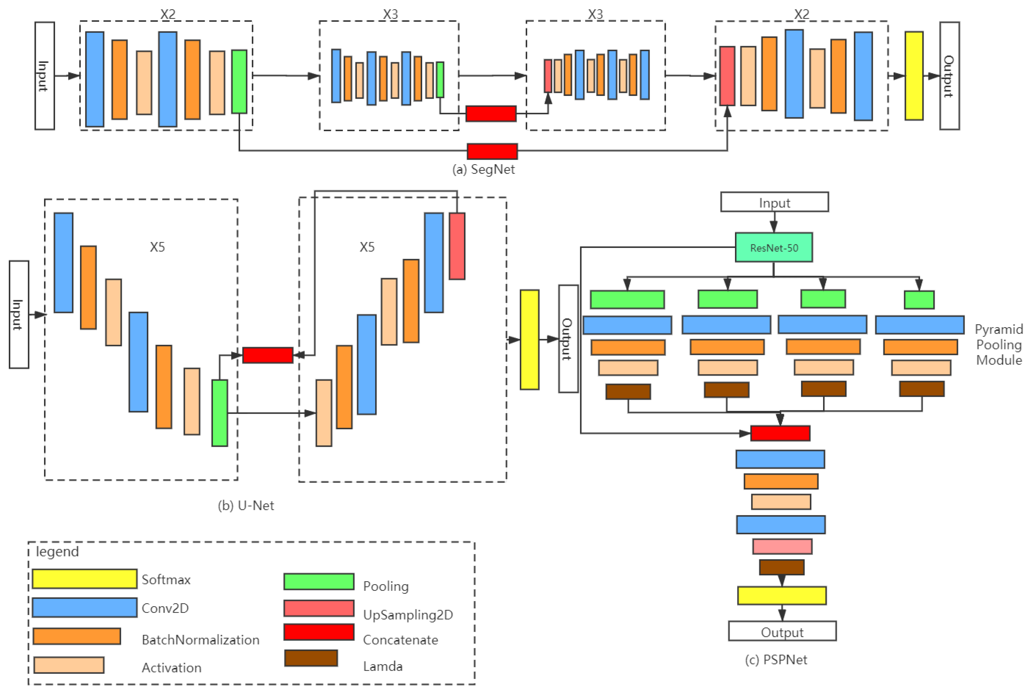
Image semantic segmentation aims to classify each pixel of an image into a category. Over the past few years, the deep-learning-based semantic segmentation classification, as a pixel-based classifier, has achieved remarkable success in image classification. It also has been used on land cover mapping with remote sensing imagery. J. Long et al. [82] were the first to develop a fully convolutional network (FCN) (containing only convolutional layers) trained end-to-end for image segmentation. Within the state-of-the-art systems, the semantic segmentation network can be divided into two categories: encoder-decoder and spatial pyramid pooling with multi-scale context design [83]. SegNet, U-Net, and PSPNet [35,36,84] were three most commonly used and comparable architectures in those two categories. In this section, we provided comprehensive descriptions to these three semantic segmentation architectures. Figure 2 illustrates their architectures. A 2D convolutional (Conv2D) layer, followed by a batch normalisation layer and an activation layer (rectified linear unit (ReLU) in this work) is the basic convolutional structure in a DCNN model to extract feature from input. Using multiple convolutional layers has been proven quite successful in improving the performance of the classification model [37]. The pooling layer was used to reduce the spatial dimensions and parameters, and to avoid over fitting. The UpSampling2D was used to recover the deep feature to the original size of input after pooling operations. There are a few different approaches that we can use to upsample the resolution of a feature map, including nearest neighbour unpooling, maximum unpooling, ConvTranspose2d [85], and PixelShuffle unpooling [86]. The PixelShuffle unpooling has a high performance on image super-resolution [87]. The Softmax layer is a function that normalises input into probability distributions of all categories and is always the last layer in a multi-class classification models. The concatenate layer is used to connect the encoder and decoder; more detailed descriptions are provided in the following section.

2.3.1. SegNet

SegNet, as shown in Figure 2a, is a combination of a fully convolutional network and an encoder- decoder architecture. In the encoding stage, the input is passed through a sequence of convolutions, ReLUs, and max-pooling layers. The output is a representation with a reduced spatial resolution. The decoding stage has the same layers as the encoder but in a reverse order. Max-pooling layers are replaced by un-pooling layers, where the values are restored to their original locations, and the convolution layers are then used to interpolate a higher-resolution image. Because the network does not have any fully connected layers (which consume >90% of parameters in a typical image-processing CNN), SegNet is highly memory efficient and comparatively easy to be trained. The SegNet architecture was originally designed for RGB-like image segmentation, such as classifying road scenes. Its input can have multi-channels and it is particularly suitable for unbalanced labels [84]. Therefore, the model is particularly suitable for remote sensing image classification; it has been applied to the classification of high-resolution remote sensing images [84,88]. As an optimised encoder-decoder pixeled based classification method, SegNet borrowed the concept of ResNet [89] in order to avoid the problem of vanishing/exploding gradients when the net became deeper, the features in the encoder stage were concatenated into the decoder stage. One study [38] used the SegNet architecture with a fusion table to classify Earth observation data (ISPRS 2D Semantic Labeling Challenge Dataset at 0.125 m resolution (Data available at: http://www2.isprs.org/commissions/comm3/wg4/semantic-labeling.html)) into five types, achieving an accuracy of 89.8%.

2.3.2. U-Net

U-Net, as shown in Figure 2b, was initially published for biomedical image segmentation. U-Net has a similar structure to SegNet; it simply concatenates the encoder feature maps to upsampled feature maps from the decoder at every stages to form a ladder-like structure. Meanwhile, the architecture with skip concatenation connections allows the decoder at each stage to learn back relevant features that are lost after pooling operations in the encoder. The architecture is simple and efficient: it consists of a contracting path to capture context and a symmetric expanding path, enabling precise localisation. It has been widely applied in Kaggle competition for building and road classification on high resolution remote sensing imagery with better accuracy [90]. One team [91] adopted the U-Net approach as their winning solution for the Spacenet Challenge and Defence Science and Technology Laboratory (Dstl) Satellite Imagery Feature Detection (Kaggle).

2.3.3. PSPNet

PSPNet, as shown in Figure 2c, using pyramid pooling modules, is one of the most advanced semantic segmentation architectures at present; it achieved first at the ImageNet Scene Parsing Challenge 2016, and 1st place on PASCAL VOC 2012 and Cityscapes datasets [92,93,94]. The PSPNet starts with a modified ResNet architecture to extract the feature information. Then, to get the multi-scale information from features maps, the spatial pyramid pooling module is introduced by applying four different maximum pooling operations with four different window sizes and strides. This effectively captures different scale feature information without heavy individual processing. Then, the deep feature information with different scales is combined and fed into the decoder. By using the spatial pyramid pooling, the features at different scales are used for classification to help improve the performance on small targets [95]. Since its launch, PSPNet has been widely used in land cover classification on medium to high remote sensing imagery [96,97].

2.4. Deep Learning-Based Object Detection for Land Cover at an Object Level

One of the most important image recognition tasks with deep learning-based methods is object detection. By detecting bounding boxes around objects and then classifying them, the object detection method at an object-level, can be used to detect and identify special objects on Earth in a large area with remote sensing imagery, especially at high to very high resolutions. The two well-known commercial remote sensing data companies, Airbus and Digital Global, have launched the object detection challenges with high resolution remote sensing imagery, encouraging users to detect and identify buildings, roads, and ships as quickly as possible by using deep learning-based methods [43,98]. Currently, the research on deep learning-based object detection can be broadly divided into two directions: multi-stage detection and single stage detection. The first one is based on the region proposal network (RPN) which usually has two stages that begin with the region search and then perform the corresponding classification. The two best performing and known models are the faster region-based convolutional network (Faster R-CNN) from Facebook [33] and Cascade R-CNN from Multimedia Laboratory, CUHK [99]. The second one is based on one-time prediction which directly predicts bounding boxes and class probabilities with a single network in a single evaluation. This allows real-time predictions. The first typical model based on one-time prediction is the you only look once (YOLO) series [100,101,102]. YOLO was designed for a fast prediction. In order to improve its accuracy, two state-of-the-art architectures were introduced by optimising the YOLO architecture: single-shot detector (SSD) [103] and RetinaNet [104]. In the past two years, these methods have been used by competition players and researchers for land cover classification. The architectures of four object detection models are shown in Figure 3. The feature map is the deep feature extracted from input by a DCNN structure. In this work, the classic Resnet50 structure was used to extract feature maps [31]. The region proposal network (RPN) was the key component in the detection model which generated the proposals for the objects in feature maps [33]. The classification and Bbox regression are the last two layers on all detection models that get the boundary and the category of the object by regression. More detailed descriptions are provided in the following section.

2.4.1. Faster R-CNN/Cascade R-CNN

Faster R-CNN is now a canonical model for deep learning-based object detection. Faster R-CNN divides the framework of detection into two stages (see Figure 3a). In the first stage, called the region proposal network (RPN), the input is processed to extract feature maps by a CNN. Then, the feature maps are used to predict bounding box proposals. In the second stage, these proposals are used to crop features from the feature maps, which are subsequently fed to the fast R-CNN for classification and B-box regression. Through comprehensive evaluations [105,106] concluded that the faster R-CNN was an efficient and robust method for object detection with high resolution remote sensing imagery, especially for small object detection. This method has also been used for the detection of large objects, such as cars, aircraft, airports, and ships [107,108,109,110].
In this two-stage object detection model, Intersection over Union (IoU) threshold is required to define positives and negatives for each region proposal in the first stage. The model trained with a low IoU produces noisy detection and a high IoU results in lossy detection. Cascade R-CNN [99] introduced a multi-stage concept by increasing IoU thresholds for each stage (see Figure 3b). It surpassed all object detectors on the challenging COCO dataset [111]. The cascade R-CNN classifier has been tested on multi-source remote sensing data, including optical, hyperspectral, and light detection and ranging (LiDAR) data, and has achieved much better classification performance than other methods [112,113]. It also has been used for aircraft and vehicle detection across large areas in high resolution imagery [114,115].

2.4.2. SSD/RetinaNet

The SSD model is designed for object detection in real-time. It is a single-stage detection model derived from the YOLO model. It has no delegated RPN and predicts the boundary boxes and the classes directly from feature maps in one single pass. To improve the accuracy, the feature maps from convolutional layers at different positions of the network are used to predict the bounding boxes (see Figure 3c). They are processed with a small 3 × 3 convolutional filter to produce a set of bounding boxes similar to the anchor boxes of the Fast R-CNN. Due to the high efficiency of single stage detector, SSD has been used to detect targets in large areas. Researchers [116,117,118] compared the performances of single stage detection method (SSD) and multi-stage detection (including faster-RCNN) regarding detecting ships, airports, and aircraft using high remote sensing imagery. The SSD achieved a significant better result in prediction speed with a similar accuracy to faster R-CNN. The SSD makes its detections from multiple feature maps. However, only the features extracted from upper layers are used for detection; the features from the bottom layers in high resolution are not used for detection due to a lack of semantic values. Therefore, it was reported that the SSD performed worse for small objects detection on high resolution imagery [119]. RetinaNet was introduced by adding a Feature Pyramid Network (FPN) construct [104] (see Figure 3d). The FPN was designed to use feature maps from both bottom and upper layers for detection, which provides a top-down pathway to construct higher resolution layers. Meanwhile, it also proposed a focal loss function trying to resolve the class imbalance effect by reducing the loss for well-trained classes. The RetinaNet showed the best performance as a single-stage detection model on COCO datasets [111]. This method was quickly used in remote sensing classification applications [120] and achieved top three in ESRI Data Science Challenge 2019 for object detection with high resolution aerial imagery [121].

3. Two Case Studies Using Deep Learning-Based Approaches

To examine the performance of deep learning-based approaches on land cover classification and objection detection, we chose the state-of-the-art deep-learning-based approaches, including semantic segmentation and object detection, and conducted experimental evaluations through two case studies, as follows:
  • Land cover classification on 5 m high resolution imagery at a pixel level. The high-quality land cover products in high spatial resolution can provide very detailed information which can be used in almost all studies on Earth’s ecosystems.
  • Wind turbine quantity and location detection on Google Earth’s imagery at an object level. The accurate location information in large areas can help researchers evaluate the impact of the rapidly growing use of wind turbines on wildlife and climate changes.

3.1. Land Cover Classification Using Deep Learning Approaches at the Pixel Level

Land cover classification is one of the most important tasks remote sensing data can be used for. As mentioned before, the increase of spatial resolution may increase the inter-class variation and decrease the inter-class variation, leading to great difficulty in using traditional classification methods for accurate classification [122]. In this section, we evaluate the performance of three state-of-the-art semantic segmentation classifiers on a real land cover task. The pixel-based traditional machine learning classifiers were also implemented for comparison.

3.1.1. Study Area

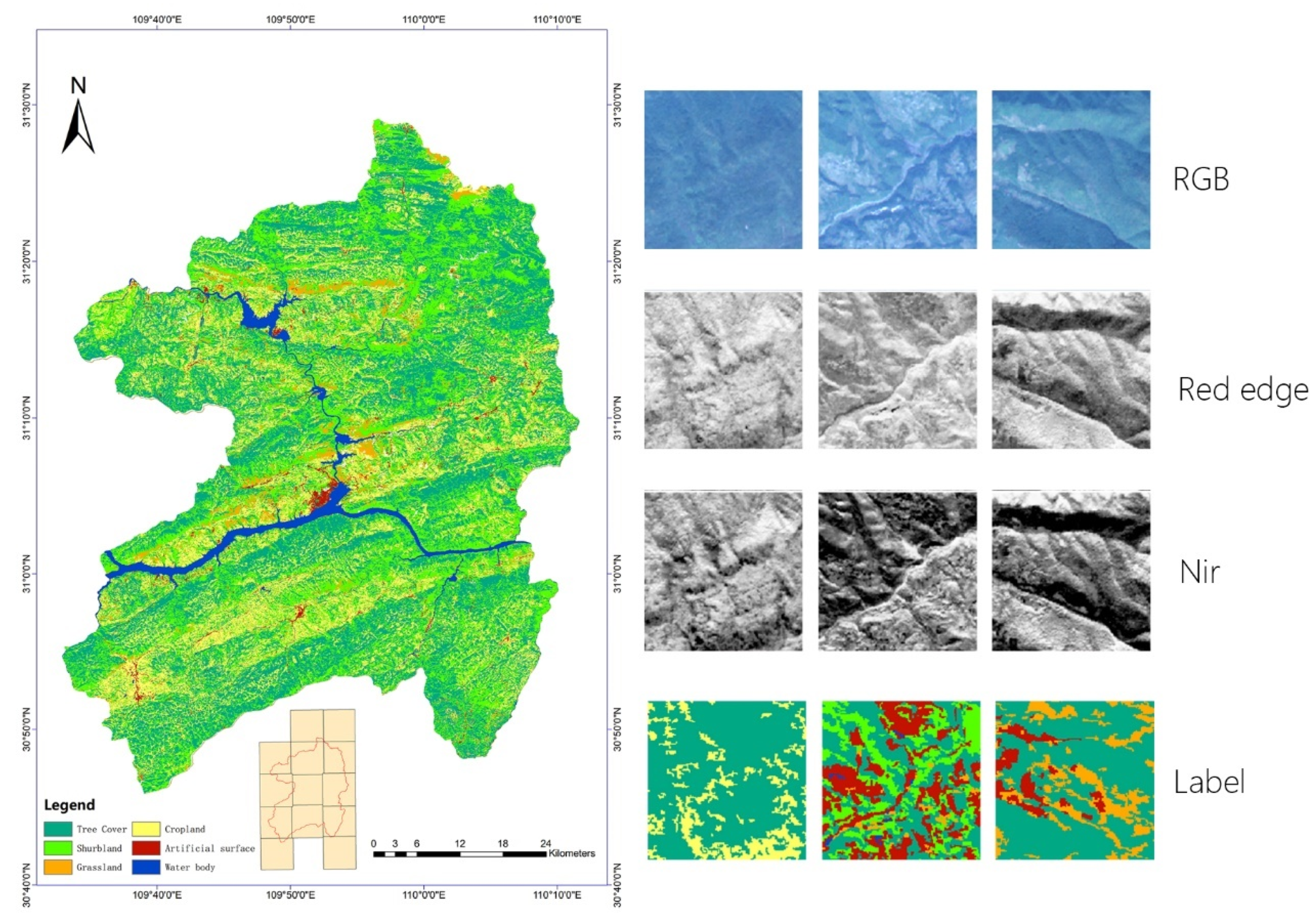
In this study, we have used a real dataset from RapidEye imagery at a 5 m resolution; the aim was to produce a land cover map with six categories, including tree cover, shrubland, grassland, cropland, artificial surface, and water body. We chose Wushan county located in Chongqing municipality, China, as the study area. The location is between E 109 ° 33 to E 110 ° 11 and N 23 ° 28 to N 30 ° 45 . Wushan is a farming-based county where most croplands are distributed around residential areas, which makes the land cover classification challenging.

3.1.2. Data Descriptions

The RapidEye images at a 5 m resolution were used in this study. The RapidEye constellation was launched into orbit on 29 August 2008. The five satellites designated herein as RE1, RE2, RE3, RE4, and RE5, were phased in a sun-synchronous orbit plane with an inclination of 97.80 ° . The RapidEye constellation sensors provide 5 meter resolution imagery in five-bands: blue (440–510 nm), green (520–590 nm), red (630–685 nm), red edge (690–730 nm), and near infrared (760–850 nm). These sensors provide abundant spatial and spectral information, which has been widely used for agriculture, forestry, environmental monitoring, and other applications. The series-unique red-edge band, which is sensitive to change in chlorophyll content, can assist in monitoring vegetation health, improving species separation, and measuring protein and nitrogen contents in biomass [123]. In this study, 13 tiles, in 2012, with the minimum cloud cover in summer and autumn, were collected (see Figure 4; data available at: https://www.planet.com/products/).

3.1.3. Performance Evaluation Metric

To evaluate the land cover classification performance, two commonly used metrics, F1-score and the confusion matrix, were selected for the accuracy assessment. Usually, neither precision nor recall can comprehensively evaluate the performance of classification. Precision measures the fraction of the identified positives that are actually positive, while Recall measures the fraction of the positives that are correctly identified. The F1-score considers both the producer’s accuracy (PA) and the user’s accuracy (UA, also called the precision and the recall) to compute the score. The study used error matrices which provided the UA, PA, and F1-score, which were calculated with the following equations:
R e c a l l ( U A ) = x i j x j × 100 %
P r e c i s i o n ( P A ) = x i j x i × 100 %
F 1 s c o r e = U A × P A U A + P A ,
where X i j represents the observation in row i, column j of confusion matrix; X i is the marginal total of row i and X j is the marginal total of column j of confusion matrix.

3.1.4. Experimental Evaluation

Data Preprocessing

Remote sensing images are usually too large to pass through a DCNN (deep convolutional neural network) under current GPU memory limitations. Most DCNNs are tailored for a resolution of 256 × 256 or 512 × 512 pixels. In this work, we split our training data into smaller patches using a simple sliding window (Figure 5). The original imagery was divided into 512 × 512 patches. Adjusting the overlap rate could increase the number of samples; hence, reducing the over-fitting. Therefore, the overlap rate was set to half of the patch size, which led to an increase of 0.5 times the samples.

Data Augmentation

The easiest and most common method to reduce over-fitting in deep learning models is to artificially enlarge the dataset using label-preserving transformations [37] i.e., data augmentation. In this study, four types of data augmentation were used for each sample, rotate 90 ° and 90 ° , flip, and mirror (Figure 6).

Model Training

We randomly selected 80% of samples for training and used the remaining portion for validation. The Adam (a method for stochastic optimisation) with a batch size of eight samples was used for optimisation in the model. We initially set a base learning rate of 1 × 10 3 .
The base learning rate was finally decreased to 1 × 10 6 following the increased iterations. A hybrid Dice and Focal loss was used in all semantic segmentation networks [124]. The Dice loss can be helpful since it boosts the prediction of correct masks, but it might lead to unstable training [125]. The focal loss [104] was proposed for solving the imbalance on the traditional cross entropy (CE) loss. The loss function in this work was defined as:
L o s s = F o c a l L o s s + ( log D i c e L o s s )
F o c a l L o s s p t = 1 p t γ log p t
D i c e L o s s = 2 × T P 2 × T P + F P + F N .
Here we use a log D i c e L o s s term in which the log operation boosts the loss for the cases when dice loss is close to zero; i.e., objects are not detected correctly. The log p t is the cross entropy (CE) loss widely used for binary classification where the p is the probability of each class. The term 1 p t in focal loss is the modulating factor added for addressing the data imbalance problem, in which γ is the focusing parameter that can be set in the range of 0–5. In this study the value of γ was set to 2, to put more focus on hardly misclassified classes. The TP, FP, and FN are true positives, false positives, and false negatives (FN), respectively. SegNet, U-Net, and PSPNet were implemented based on the pytorch 0.41 and executed on a PC with an Intel (R) Xeon (R) CPU E5-2650, NVIDIA TITAN X (Pascal) and 64GB memory.

3.1.5. Experimental Results

Three semantic segmentation deep learning methods, including SegNet, U-Net, PSPNet, and three pixel-based traditional machine learning methods, were evaluated. The F1 score for each method across categories is shown in Figure 7. For traditional machine learning methods, the RF has the best performance for all categories. In most instances, the results based on deep learning methods are better than those based on traditional machine learning methods. In this work, the F1 score values based on SegNet and U-Net are higher than those based on pixel-based traditional methods, especially when detecting shrubland, grassland, cropland, and artificial surface. For most categories, the two methods have similar performances in terms of F score, although U-Net performs slightly better than SegNet. The F1 score measure shows the superiority of this model. PSPNet performs significantly better than other models, especially on detecting shrubland and grassland in terms of F-score. Ensemble learning, a common trick in machine and deep learning, is the process of creating multiple models and combining them through averaging the results of all the models, in order to achieve better performance than each individual model [126]. In this work, we made an ensemble of SegNet, U-Net, and PSPNet; the ensemble results were the best for most categories except grassland, as shown in Figure 7. Figure 8 shows the classification confusion matrices for SegNet, U-Net, PSPNet and the ensemble models. The water body is the most easily identifiable category due to its spectral properties. The tree cover, shrubland, grassland, cropland, and artificial surface have similar spectral properties, which make it difficult to separate them from each other. The detection results on the grassland are the poorest, and the vast majority of pixels in the region of grassland are assigned to shrubland and cropland. Meanwhile, many pixels belonging to artificial surface are assigned to croplands. The reason behind is that Wushan is a farming-based county where most croplands are distributed around residential areas which are hard to be identified. Another reason is that most images were acquired in summer and autumn when most croplands were near harvest or after harvest. Some bare croplands after harvest are assigned as artificial surface.

3.2. Land Cover Object Detection Using Deep Learning Approaches at an Object Level

The second case study aimed to identify wind turbine location and quantity automatically. The previous studies [127,128,129] have shown that the wind turbine influenced the local climate. Wind turbines can modify the surface fluxes of momentum, sensible heat, water vapor, and carbon dioxide by enhancing turbulence, increasing surface roughness, and changing the stability of the atmospheric boundary layer. Meanwhile, there was evidence that the turbine locations could affect the living habits of wildlife [130,131]. We applied the widely used single-stage and multi-stage object detection models to wind turbine detection and evaluated their performance.

3.2.1. Study Area

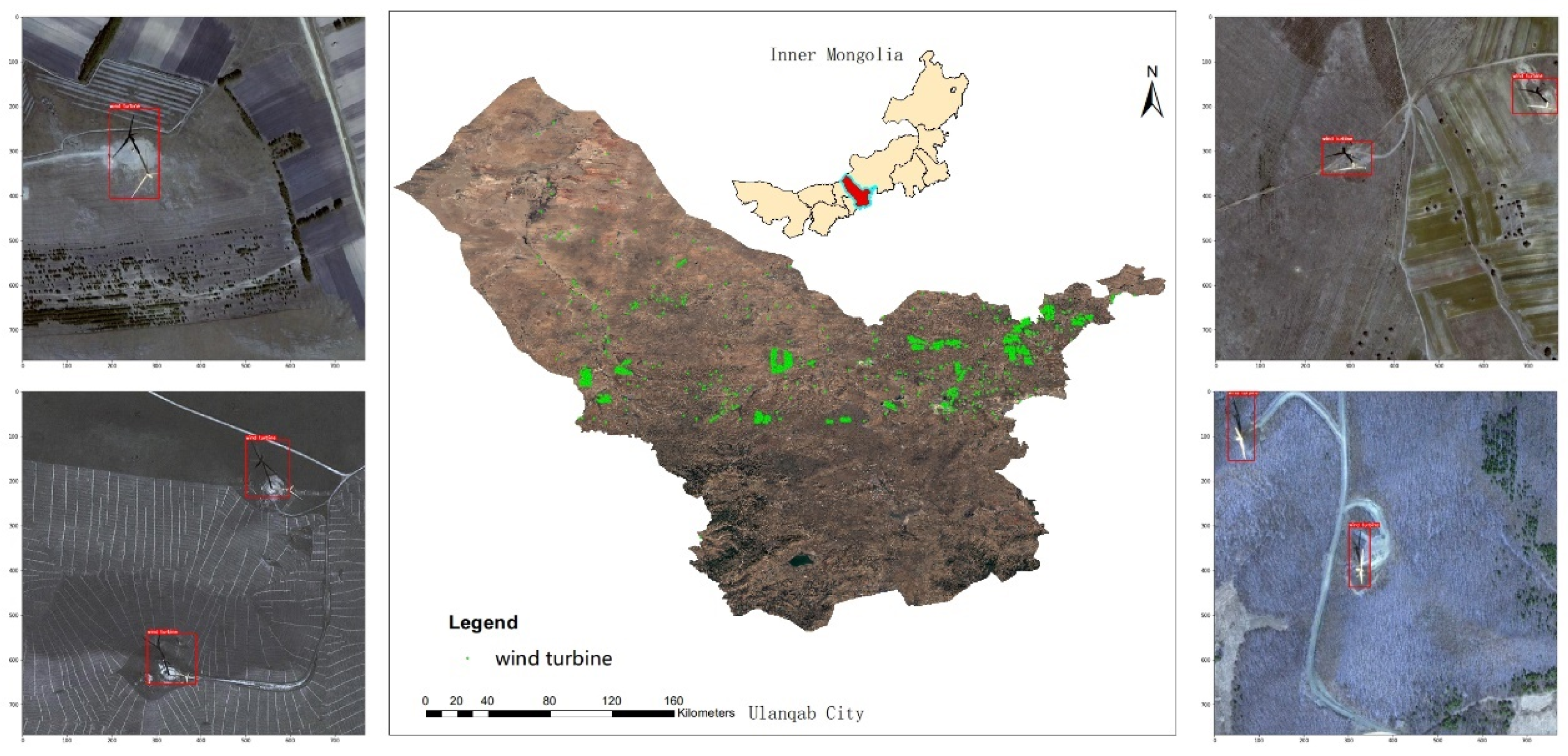
Due to the rapid expansion of demand for energy and the rapid development of wind power facility in recent years, a great number of wind turbines have been built in China [132]. According to statistical results of the wind energy resource survey, China’s onshore wind power energy reserve from 10 m in height is about 4.35 billion kilowatts, ranked first in the world [133]. Inner Mongolia is located in the north of the country. It occupies approximately 1,183,000 km 2 , which is the third largest Chinese subdivision in China. Inner Mongolia’s exploitable wind resources account for about half of the country’s total amount, and its wind energy utilisation area accounts for 80% of the total area. In this paper, Inner Mongolia was selected as the study area.

3.2.2. Data Description

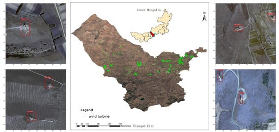
The size of the wind turbine determines that only high-resolution remote sensing data can be used for identification. The WorldView image with the spatial resolutions ranging from 0.5 m to 2 m in whole Inner Mongolia were captured from Google Earth images. Due to technical limitations, only visible RGB bands were acquired for this work. We labelled the locations of a total of 13,391 wind turbines in the Ulanqab city through the Google Earth pro [134]. The bound box of each wind turbine was annotated by LabelMe [135]. Some examples of labelled images are shown in Figure 9.

3.2.3. Performance Evaluation Metric

The commonly used metric for object detection challenges is the mean average precision (mAP). It is the mean of the average precisions (APs) for all classes. The AP is computed as the average of maximum precision at 11 recall levels of 0.0, 0.1 m, , 1.0, defined as:
m A P = 1 11 × A P r 0 + A P r 0.1 + A P r 0.2 + + A P r 1 ,
where A P r 0 means the maximum precision at the recall level of 0. Only one class (wind turbine) was required for identification, and AP was selected for evaluating the wind turbine performance. If the AP matched the ground truth, and intersection over union (IOU) was above 0.5, then the object detection detection was considered successful. Meanwhile, when detecting the object went across the whole study area with high resolution images, more than 1,300,000 images with 512 × 512 resolution need to be inferred. Therefore, the inference time (fps) indicating how many images can be inferred per second was also selected as a metric for performance evaluation.

3.2.4. Experimental Evaluation

The same data preprocessing as used in Section 3.1 was performed, including sliding window and data augmentation. The high-resolution images from Google Earth were cut into 512 × 512 as the model input. All the models were trained and validated on a dataset of 8738 images, with 13,391 wind turbines. We randomly selected 80% of samples for training and used the rest to evaluate the performance of the deep learning-based object detection network.

Model Training

All the object detection models, including two multi-stage detection models (faster and cascade R-CNN) and two single stage detection models (SSD and RetinaNet) were implemented and trained with mmdetection, an open source object detection toolbox based on PyTorch [136]. The Resnet50 with pretrained weights from ImageNet was set as the backbone in detection models. The stochastic gradient descent (SGD) with a batch size of eight was used for optimisation. We initially set a base learning rate of 1 × 10 3 . The base learning rate was finally decreased to 1 × 10 6 following the iterations, and each model was trained for 24 epochs.

Post Processing

An aggregated polygon method was used after the prediction. As shown in Figure 10, multiple overlapping detected bounding boxes appear on images for one object after sliding window operations. On one hand, we used the slide window method with an overlap rate of 0.5 in the prediction stage to make each wind turbine appear on the input images completely; hence, one wind turbine appearing on multiple images could be identified multiple times. On the other hand, the model might also identify parts of a wind turbine as an object. An aggregated algorithm was used to merge the overlapping and closed detected bounding boxes.

Experimental Results

Table 1 lists a performance comparison of different methods. In terms of detection accuracy measured by the AP value, the four models are close; all have a value of above 0.90. The model based on Cascade R-CNN has the highest AP value before and after polygon aggregation. After aggregating the closed and overlapping detected bounding boxes, the AP values from all models are increased significantly. For the cascade-R-CNN, the AP value reaches to 0.988. In terms of inference speed measured by impressive frame per second (FPS) and inference time, the single-stage detectors, SSD and RetinaNet, perform better than the two multi-stage detectors, faster R-CNN and cascade R-CNN. The SSD based model can infer 29.5 images per second and is 0.5 times faster than the cascade R-CNN based model, even if their AP performance values are close.
Figure 11 shows typical object detection results in different areas with the Cascade R-CNN approach. A green colour box represents a correctly detected object and a red box represents a false detection. All the object detection models in this work show a high AP accuracy, and almost all the wind turbine can be well detected. However, the current trained models still falsely detect some objects with similar morphological and texture features (such as light and crossroads) as wind turbines. Although we can increase the detection precision of models by raising the detection threshold, it will cause some omissions. If the goal of remote sensing object detection is to detect all targets, this strategy is not recommended.
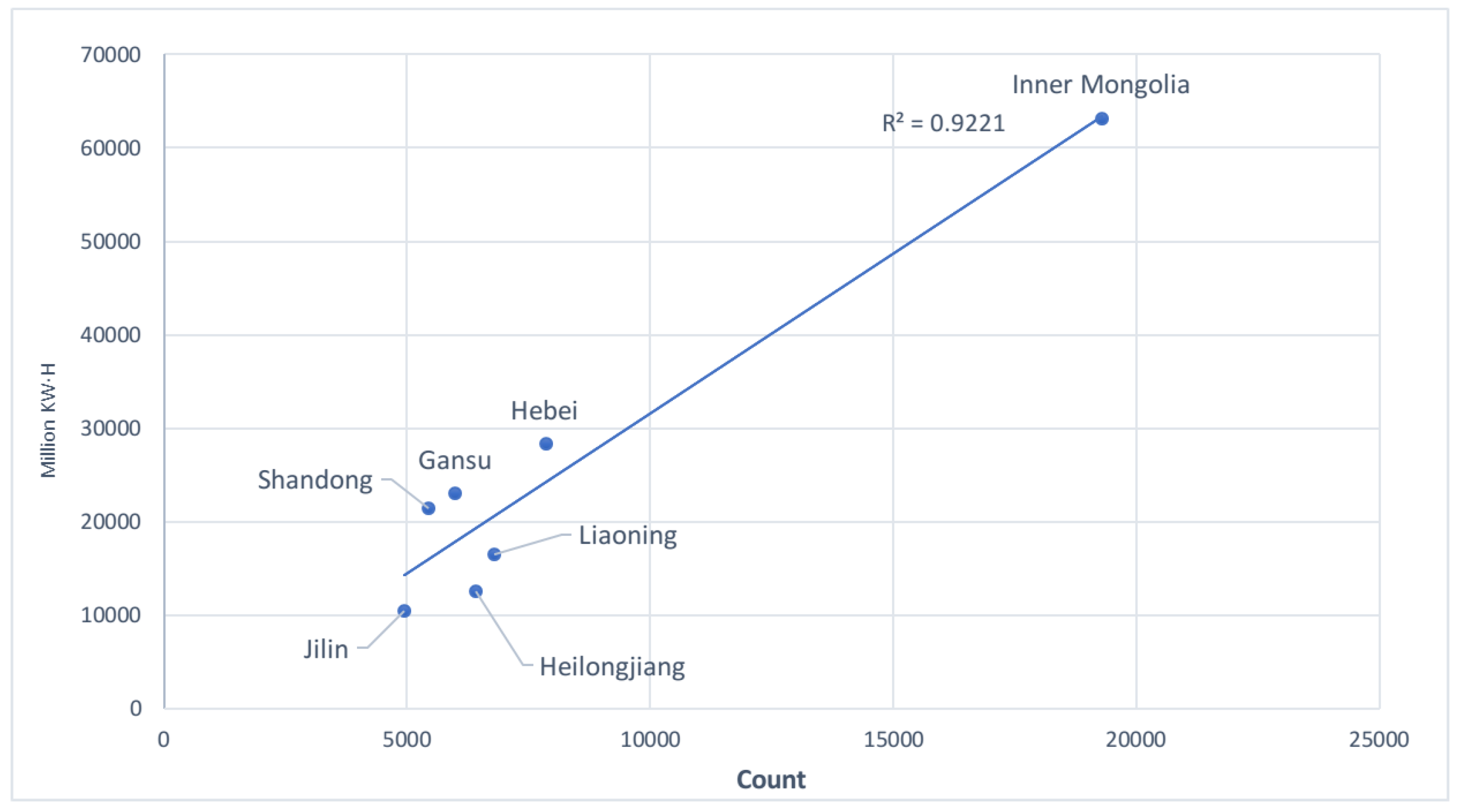
At last, we tested the robustness of the model in a large area. We applied the detection model to the seven largest power generation provinces in China, and compared the relationship between the wind power generation and the number of wind turbines (Inner Mongolia, Hebei, Gansu, Shandong, Liaoning, Heilongjiang, and Jilin). The data of wind power generation in 2018 were obtained from the National Bureau of Statistics (data available at: http://www.gov.cn/xinwen/2019-01/29/content_5361945.htm). The results are shown in Figure 12. There is a good correlation between the number of wind turbines and the wind power generation; the R 2 value reaches 0.92.

4. Discussion

In previous sections, we evaluated the performance of existing deep-learning-based approaches on high resolution images at both pixel and object levels using two case studies. Results showed that deep-learning-based methods in our cases performed better than traditional algorithms. In this section, we discuss the results and highlight the future trends.

4.1. Land Cover Classification

In traditional pixel-based classification methods, only spectral information of each pixel was used in classification. The categories with similar spectral information were difficult to classify. However, the convolution layer (see Figure 13) in all deep learning models can deal with joint spatial and spectral information with a convolution kernel. It has been proven to improve the accuracy of classification, especially in hyperspectral image classification [137,138,139]. As shown in Figure 14, the vegetation categories, including tree cover, grassland, and cropland, have similar/close spectral information. This can explain why the accuracy of deep-learning-based methods is higher than traditional methods in our land cover classification task.
Previous studies [140] showed that the classification results might appear messy visually when a pixel-based method was used for the land cover classification in medium to high resolutions. That was also true in this study. Figure 15 shows a comparison of land cover classification results between the random forest and the ensemble average of SegNet, U-Net, and PSPNet on the data at 5 m resolution. The classification results of the random forest, a traditional pixel-based method, visually, do not look good, and a severe “salt and pepper” effect appears. However, in deep learning-based classification methods, the effect can be reduced through the convolution and pooling layers. The pooling is a down-sampling process to extract the average or maximum value in an adjacent area [141] which can remove the anomalous pixels in a category. In this study, ensemble average results based on the three deep learning methods visually look much smoother, and are much closer to reality.
Further, we compared the segmentation results of a traditional segmentation method with an object-based approach and the deep learning-based method by making the ensemble of the SegNet, U-Net, and PSPNet, as shown in Figure 16. The multi-resolution segmentation algorithm [20] is the most widely used segmentation method dealing with high resolution remote sensing imagery and is integrated in eCognition Land Cover Mapping Software. In this paper, the multi-resolution segmentation algorithm was selected as a typical representative of traditional objective-based method. Considering the size of the remote sensing images and limitations of computing power, the scale level could not be too small to avoid producing too many objects; thus, a scale size of 30 for the 5 m resolution images was used. Figure 16 illustrates typical segmentation results of the two methods. As shown in the second column, the edge of each object segmented looks rough due to the scale effect of segmentation in the multi-resolution segmentation algorithm. However, the segmentation results of the deep learning-based method are smoother and more realistic from the visual aspect.
The semantic segmentation classification method showed good performance in our experiments because it can ease the limitations of current pixel-based and object-based classification methods when dealing with high-resolution images. Large-scale deep learning networks usually have over ten million parameters to be learned; Table 2 lists the parameters of the three deep learning models used in this study. Training a deep learning model with a small dataset often leads to over-fitting, decreasing the model’s generalisation ability. Although some works have chosen to use a shallow model to avoid over-fitting, this kind of choice inevitably makes the model orient toward the training data [142,143]. The transfer learning technology and a finely-tuned model can be used to reduce this effect [144]. However, the current transfer learning weights were mostly based on ImageNet, which was a regular electric-optical photo dataset [37]. Remote sensing data is often captured with multi-spectral sensors, making these weights meaningless. Although there are already some public high-resolution land cover productions for training [145,146], these public datasets are far from enough, given the complexities of remote sensing data, such as the various types of sensor, acquisition time, and spatial resolution.

4.2. Land Cover Object Detection

In object detection tasks, this the limitation of ImageNet for transfer learning can be alleviated because most of high-resolution images used in object detection work are in RGB bands. The transfer learning and fine-tune methods can be used to accelerate model fitting. In this study on object detection, parameters of Resnet50 pretrained on ImageNet were employed as initial parameters, and all the model converged in 12 epochs. By using the state-of-the-art deep learning-based object detection architectures and a GIS aggregate method, all the models achieved more than 98% accuracy. We predicted the numbers and the locations of wind turbines in seven largest power generation provinces in China in less than two weeks, including the time of removing misidentified data by visual interpretation, which was impossible with traditional methods. Meanwhile, thanks to the SpaceNet competition [147] which provides a corpus of labelled commercial satellite imagery in m-level solutions, the deep learning-based methods achieved great success on the building detection. Microsoft also used a deep-learning-based method to generate 125,192,184 building footprints in all 50 US states [148]. These results have proven that deep learning algorithms have great potential for object detection in remote sensing applications.

5. Conclusions

In this paper, we have reviewed the current, commonly used land cover mapping methods, including land cover classification and object detection methods based on high resolution images. We have examined the performance of existing state-of-the-art deep learning architectures on high resolution image for land cover classification and object detection tasks against traditional methods through two application case studies: land cover classification and wind turbine object detection. Based on the experimental evaluation, we conclude:
  • For land cover classification, the state of the art semantic segmentation deep-learning-based methods at a pixel level performed better than the pixel-based classification methods using traditional machine learning approaches through leveraging spatial information in convolution layer. Meanwhile, from the visual aspect, the segmentation results based on the deep learning method produced a visually appealing generalised appearance of land cover better than that from one of the most widely used object-based segmentation methods.
  • Considering the diversity of remote sensing data, most land cover studies on high-resolution imagery have limited training data sets, which reduces the robustness of a deep learning-based model. The deep learning-based model cannot completely replace the traditional pixel-based methods in practice.
  • A satisfying evaluation result was achieved for the current state-of-the-art deep learning-based models for a real object detection task. The deep learning-based models could relieve the burden of the traditional, labour-intensive objective detection task.

Author Contributions

Conceptualisation: all authors; methodology: X.Z. and L.H. (Liangxiu Han) and L.H. Lianghao Han); data acquisition: X.Z. and L.Z. (Liang Zhu); software: X.Z.; analysis: X.Z., L.H. (Liangxiu Han) and L.H. (Lianghao Han); writing—original draft preparation: X.Z.; writing—review and editing: all authors; supervision: L.H. (Liangxiu Han). All authors have read and agreed to the published version of the manuscript.

Funding

This research was supported Agri-Tech in the China Newton Network+ (ATCNN)—Quzhou Integrated Platform (QP003), BBSRC (BB/R019983/1), BBSRC (BB/S020969/1). The work is also supported by Newton Fund Institutional Links grant, ID 332438911, under the Newton-Ungku Omar Fund partnership (the grant is funded by the UK Department of Business, Energy, and Industrial Strategy (BEIS) and the Malaysian Industry-Government Group for High Technology and delivered by the British Council. For further information, please visit www.newtonfund.ac.uk).

Acknowledgments

We thank the anonymous reviewers for reviewing the manuscript and providing comments to improve the manuscript.

Conflicts of Interest

The authors declare no conflict of interest.

References

  1. Rawat, J.S.; Kumar, M. Monitoring land use/cover change using remote sensing and GIS techniques: A case study of Hawalbagh block, district Almora, Uttarakhand, India. Egypt. J. Remote Sens. Space Sci. 2015, 18, 77–84. [Google Scholar] [CrossRef] [Green Version]
  2. Ban, Y.; Gong, P.; Giri, C. Global land cover mapping using Earth observation satellite data: Recent progresses and challenges. ISPRS J. Photogramm. Remote Sens. 2015, 103, 1–6. [Google Scholar] [CrossRef] [Green Version]
  3. Feddema, J.J. The Importance of Land-Cover Change in Simulating Future Climates. Science 2005, 310, 1674–1678. [Google Scholar] [CrossRef] [Green Version]
  4. Duro, D.C.; Franklin, S.E.; Dubé, M.G. A comparison of pixel-based and object-based image analysis with selected machine learning algorithms for the classification of agricultural landscapes using SPOT-5 HRG imagery. Remote Sens. Environ. 2012, 118, 259–272. [Google Scholar] [CrossRef]
  5. Schowengerdt, R.A. CHAPTER 9—Thematic Classification. In Remote Sensing, 3rd ed.; Academic Press: Burlington, NJ, USA, 2007. [Google Scholar] [CrossRef]
  6. Chasmer, L.; Hopkinson, C.; Veness, T.; Quinton, W.; Baltzer, J. A decision-tree classification for low-lying complex land cover types within the zone of discontinuous permafrost. Remote Sens. Environ. 2014, 143, 73–84. [Google Scholar] [CrossRef]
  7. Friedl, M.A.; Brodley, C.E. Decision tree classification of land cover from remotely sensed data. Remote Sens. Environ. 1997, 61, 399–409. [Google Scholar] [CrossRef]
  8. Hua, L.; Zhang, X.; Chen, X.; Yin, K.; Tang, L. A Feature-Based Approach of Decision Tree Classification to Map Time Series Urban Land Use and Land Cover with Landsat 5 TM and Landsat 8 OLI in a Coastal City, China. Int. J. Geo-Inf. 2017, 6, 331. [Google Scholar] [CrossRef] [Green Version]
  9. Melgani, F.; Bruzzone, L. Classification of hyperspectral remote sensing images with support vector machines. IEEE Trans. Geosci. Remote Sens. 2004, 42, 1778–1790. [Google Scholar] [CrossRef] [Green Version]
  10. Benz, U.C.; Hofmann, P.; Willhauck, G.; Lingenfelder, I.; Heynen, M. Multi-resolution, object-oriented fuzzy analysis of remote sensing data for GIS-ready information. ISPRS J. Photogramm. Remote Sens. 2004, 58, 239–258. [Google Scholar] [CrossRef]
  11. Munoz-Mari, J.; Bovolo, F.; Gomez-Chova, L.; Bruzzone, L.; Camp-Valls, G. Semisupervised One-Class Support Vector Machines for Classification of Remote Sensing Data. IEEE Trans. Geosci. Remote Sens. 2010, 48, 3188–3197. [Google Scholar] [CrossRef] [Green Version]
  12. Beijma, S.V.; Comber, A.; Lamb, A. Random forest classification of salt marsh vegetation habitats using quad-polarimetric airborne SAR, elevation and optical RS data. Remote Sens. Environ. 2014, 149, 118–129. [Google Scholar] [CrossRef]
  13. Khatami, R.; Mountrakis, G.; Stehman, S.V. A meta-analysis of remote sensing research on supervised pixel-based land-cover image classification processes: General guidelines for practitioners and future research. Remote Sens. Environ. 2016, 177, 89–100. [Google Scholar] [CrossRef] [Green Version]
  14. Dean, A.M.; Smith, G.M. An evaluation of per-parcel land cover mapping using maximum likelihood class probabilities. Int. J. Remote Sens. 2003, 24, 2905–2920. [Google Scholar] [CrossRef]
  15. Blaschke, T.; Lang, S.; Lorup, E.; Strobl, J.; Zeil, P. Object-Oriented Image Processing in an Integrated GIS/Remote Sensing Environment and Perspectives for Environmental Applications. Environ. Inf. Plan. Politics Public 2000, 2, 555–570. [Google Scholar]
  16. Blaschke, T. Object based image analysis for remote sensing. ISPRS J. Photogramm. Remote Sens. 2010, 65, 2–16. [Google Scholar] [CrossRef] [Green Version]
  17. Weih, R.C.; Riggan, N.D. Object-Based Classification vs. Pixel-Based Classification: Comparitive Importance of Multi-Resolution Imagery. Int. Arch. Photogramm. Remote Sens. Spat. Inf. Sci. 2010, 38, C7. [Google Scholar]
  18. Whiteside, T.G.; Boggs, G.S.; Maier, S.W. Comparing object-based and pixel-based classifications for mapping savannas. Int. J. Appl. Earth Obs. Geoinf. 2011, 13, 884–893. [Google Scholar] [CrossRef]
  19. Zhang, L.; Li, X.; Yuan, Q.; Liu, Y. Object-based approach to national land cover mapping using HJ satellite imagery. J. Appl. Remote Sens. 2014, 8, 083686. [Google Scholar] [CrossRef]
  20. Ding, X.Y. The Application of eCognition in Land Use Projects. Geomat. Spat. Inf. Technol. 2005, 28, 116–120. [Google Scholar]
  21. Blaschke, T.; Burnett, C.; Pekkarinen, A. Image segmentation methods for object-based analysis and classification. In Remote Sensing Image Analysis: Including the Spatial Domain; Springer: Dordrecht, The Netherlands, 2004; pp. 211–236. [Google Scholar]
  22. Burnett, C.; Blaschke, T. A multi-scale segmentation/object relationship modelling methodology for landscape analysis. Ecol. Model. 2003, 168, 233–249. [Google Scholar] [CrossRef]
  23. Adams, R.; Bischof, L. Seeded Region Growing. IEEE Trans. Pattern Anal. Mach. Intell. 1994, 16, 641–647. [Google Scholar] [CrossRef] [Green Version]
  24. Tilton, J.C. Image segmentation by region growing and spectral clustering with a natural convergence criterion. In Proceedings of the IGARSS’98. Sensing and Managing the Environment. 1998 IEEE International Geoscience and Remote Sensing. Symposium Proceedings. (Cat. No.98CH36174), Seattle, WA, USA, 6–10 July 1998; Volume 4, pp. 1766–1768. [Google Scholar]
  25. Baatz, M.; Schäpe, A. An optimization approach for high quality multi-scale image segmentation. In Proceedings of the Beiträge zum AGIT-Symposium, Salzburg, Austria, July 2000; pp. 12–23. [Google Scholar]
  26. Roerdink, J.B.; Meijster, A. The watershed transform: Definitions, algorithms and parallelization strategies. Fundam. Inform. 2000, 41, 187–228. [Google Scholar] [CrossRef] [Green Version]
  27. Audebert, N.; Boulch, A.; Randrianarivo, H.; Le Saux, B.; Ferecatu, M.; Lefevre, S.; Marlet, R. Deep learning for urban remote sensing. In Proceedings of the 2017 Joint Urban Remote Sensing Event (JURSE), Dubai, UAE, 6–8 March 2017; IEEE: Dubai, UAE, 2017; pp. 1–4. [Google Scholar]
  28. Contreras, D.; Blaschke, T.; Tiede, D.; Jilge, M. Monitoring recovery after earthquakes through the integration of remote sensing, GIS, and ground observations: The case of L’Aquila (Italy). Cartogr. Geogr. Inf. Sci. 2016, 43, 115–133. [Google Scholar] [CrossRef]
  29. Nebiker, S.; Lack, N.; Deuber, M. Building Change Detection from Historical Aerial Photographs Using Dense Image Matching and Object-Based Image Analysis. Remote Sens. 2014, 6, 8310–8336. [Google Scholar] [CrossRef] [Green Version]
  30. Li, X.; Myint, S.W.; Zhang, Y.; Galletti, C.; Zhang, X.; Turner, B.L. Object-based land-cover classification for metropolitan Phoenix, Arizona, using aerial photography. Int. J. Appl. Earth Obs. Geoinf. 2014, 33, 321–330. [Google Scholar] [CrossRef]
  31. He, K.; Zhang, X.; Ren, S.; Sun, J. Deep residual learning for image recognition. In Proceedings of the IEEE Conference on Computer Vision and Pattern Recognition, Las Vegas, NV, USA, 26 June–1 July 2016; pp. 770–778. [Google Scholar]
  32. Szegedy, C.; Ioffe, S.; Vanhoucke, V.; Alemi, A.A. Inception-v4, inception-resnet and the impact of residual connections on learning. In Proceedings of the Thirty-First AAAI Conference on Artificial Intelligence, San Francisco, CA, USA, 4–10 February 2017. [Google Scholar]
  33. Ren, S.; He, K.; Girshick, R.; Sun, J. Faster R-CNN: Towards Real-Time Object Detection with Region Proposal Networks. arXiv 2015, arXiv:1506.01497. [Google Scholar] [CrossRef] [Green Version]
  34. Redmon, J.; Divvala, S.; Girshick, R.; Farhadi, A. You only look once: Unified, real-time object detection. In Proceedings of the IEEE Conference on Computer Vision and Pattern Recognition, Las Vegas, NV, USA, 26 June–1 July 2016; pp. 779–788. [Google Scholar]
  35. Ronneberger, O.; Fischer, P.; Brox, T. U-Net: Convolutional Networks for Biomedical Image Segmentation. In International Conference on Medical Image Computing and Computer-Assisted Intervention; Springer: Cham, Switzerland, 2015; pp. 234–241. [Google Scholar]
  36. Zhao, H.; Shi, J.; Qi, X.; Wang, X.; Jia, J. Pyramid Scene Parsing Network. In Proceedings of the IEEE Conference on Computer Vision and Pattern Recognition, Las Vegas, NV, USA, 26 June–1 July 2016. [Google Scholar]
  37. Krizhevsky, A.; Sutskever, I.; Hinton, G.E. ImageNet classification with deep convolutional neural networks. In Proceedings of the Advances in Neural Information Processing Systems, Lake Tahoe, NV, USA, 3–6 December 2012; pp. 1097–1105. [Google Scholar]
  38. Audebert, N.; Saux, B.L.; Lefèvre, S. Semantic Segmentation of Earth Observation Data Using Multimodal and Multi-scale Deep Networks. arXiv 2016, arXiv:1609.06846. [Google Scholar]
  39. Huang, B.; Zhao, B.; Song, Y. Urban land-use mapping using a deep convolutional neural network with high spatial resolution multispectral remote sensing imagery. Remote Sens. Environ. 2018, 214, 73–86. [Google Scholar] [CrossRef]
  40. Kemker, R.; Salvaggio, C.; Kanan, C. Algorithms for Semantic Segmentation of Multispectral Remote Sensing Imagery using Deep Learning. ISPRS J. Photogramm. Remote Sens. 2018, 145, 60–77. [Google Scholar] [CrossRef] [Green Version]
  41. Zheng, C.; Wang, L. Semantic Segmentation of Remote Sensing Imagery Using Object-Based Markov Random Field Model With Regional Penalties. IEEE J. Sel. Top. Appl. Earth Obs. Remote Sens. 2015, 8, 1924–1935. [Google Scholar] [CrossRef]
  42. Van Etten, A. You Only Look Twice: Rapid Multi-Scale Object Detection In Satellite Imagery. arXiv 2018, arXiv:1805.09512. [Google Scholar]
  43. Van Etten, A. Satellite Imagery Multiscale Rapid Detection with Windowed Networks. arXiv 2018, arXiv:1809.09978. [Google Scholar]
  44. Congalton, R.G.; Gu, J.; Yadav, K.; Thenkabail, P.; Ozdogan, M. Global Land Cover Mapping: A Review and Uncertainty Analysis. Remote Sens. 2014, 6, 12070–12093. [Google Scholar] [CrossRef] [Green Version]
  45. Rogan, J.; Chen, D. Remote sensing technology for mapping and monitoring land-cover and land-use change. Prog. Plan. 2004, 61, 301–325. [Google Scholar] [CrossRef]
  46. Bartholome, E.; Belward, A.S. GLC2000: A new approach to global land cover mapping from Earth observation data. Int. J. Remote Sens. 2005, 26, 1959–1977. [Google Scholar] [CrossRef]
  47. Bontemps, S.; Defourny, P.; Bogaert, E.V.; Arino, O.; Kalogirou, V.; Perez, J.R. GLOBCOVER 2009-Products Description and Validation Report. 2011. Available online: https://epic.awi.de/id/eprint/31014/16/GLOBCOVER2009_Validation_Report_2-2.pdf (accessed on 28 April 2019).
  48. Hansen, M.C.; Defries, R.S.; Townshend, J.R.G.; Sohlberg, R. Global land cover classification at 1 km spatial resolution using a classification tree approach. Int. J. Remote Sens. 2000, 21, 1331–1364. [Google Scholar] [CrossRef]
  49. Li, W.; Ciais, P.; MacBean, N.; Peng, S.; Defourny, P.; Bontemps, S. Major forest changes and land cover transitions based on plant functional types derived from the ESA CCI Land Cover product. Int. J. Appl. Earth Obs. Geoinf. 2016, 47, 30–39. [Google Scholar] [CrossRef]
  50. Mora, B.; Tsendbazar, N.E.; Herold, M.; Arino, O. Global Land Cover Mapping: Current Status and Future Trends; Springer: Dordrecht, The Netherlands, 2014. [Google Scholar]
  51. Fritz, S.; See, L. Identifying and quantifying uncertainty and spatial disagreement in the comparison of Global Land Cover for different applications. Glob. Chang. Biol. 2008, 14, 1057–1075. [Google Scholar] [CrossRef]
  52. Herold, M.; Mayaux, P.; Woodcock, C.E.; Baccini, A.; Schmullius, C. Some challenges in global land cover mapping: An assessment of agreement and accuracy in existing 1 km datasets. Remote Sens. Environ. 2008, 112, 2538–2556. [Google Scholar] [CrossRef]
  53. Latifovic, R.; Olthof, I. Accuracy assessment using sub-pixel fractional error matrices of global land cover products derived from satellite data. Remote Sens. Environ. 2004, 90, 153–165. [Google Scholar] [CrossRef]
  54. Hansen, M.C.; Loveland, T.R. A review of large area monitoring of land cover change using Landsat data. Remote Sens. Environ. 2012, 122, 66–74. [Google Scholar] [CrossRef]
  55. Malenovskỳ, Z.; Rott, H.; Cihlar, J.; Schaepman, M.E.; García-Santos, G.; Fernandes, R.; Berger, M. Sentinels for science: Potential of Sentinel-1,-2, and-3 missions for scientific observations of ocean, cryosphere, and land. Remote Sens. Environ. 2012, 120, 91–101. [Google Scholar] [CrossRef]
  56. Dial, G.; Bowen, H.; Gerlach, F.; Grodecki, J.; Oleszczuk, R. IKONOS satellite, imagery, and products. Remote Sens. Environ. 2003, 88, 23–36. [Google Scholar] [CrossRef]
  57. Chevrel, M.; Courtois, M.; Weill, G. The SPOT satellite remote sensing mission. Photogramm. Eng. Remote Sens. 1981, 47, 1163–1171. [Google Scholar]
  58. Pádua, L.; Vanko, J.; Hruška, J.; Ad ao, T.; Sousa, J.J.; Peres, E.; Morais, R. UAS, sensors, and data processing in agroforestry: A review towards practical applications. Int. J. Remote Sens. 2017, 38, 2349–2391. [Google Scholar] [CrossRef]
  59. Feng, Q.; Liu, J.; Gong, J. UAV Remote Sensing for Urban Vegetation Mapping Using Random Forest and Texture Analysis. Remote Sens. 2015, 7, 1074–1094. [Google Scholar] [CrossRef] [Green Version]
  60. Bruzzone, L.; Prieto, D.F. Unsupervised retraining of a maximum likelihood classifier for the analysis of multitemporal remote sensing images. IEEE Trans. Geosci. Remote Sens. 2001, 39, 456–460. [Google Scholar] [CrossRef] [Green Version]
  61. Congalton, R.G. A review of assessing the accuracy of classifications of remotely sensed data. Remote Sens. Environ. 1991, 37, 35–46. [Google Scholar] [CrossRef]
  62. Ball, G.H.; Hall, J. ISODATA: A Novel Method for Data Analysis and Pattern Classification; Stanford Research Institute: Menlo Park, CA, USA, 1965. [Google Scholar]
  63. Kanungo, T.; Mount, D.; Netanyahu, N.; Piatko, C.; Silverman, R.; Wu, A. An efficient k-means clustering algorithm: Analysis and implementation. IEEE Trans. Pattern Anal. Mach. Intell. 2002, 24, 881–892. [Google Scholar] [CrossRef]
  64. ENVI. ENVI User’s Guide. In ITT Visual Information Solutions; ENVI, 2008; Available online: http://www.harrisgeospatial.com/portals/0/pdfs/envi/ENVI_User_Guide.pdf (accessed on 28 April 2019).
  65. Melesse, A.M.; Jordan, J.D. A comparison of fuzzy vs. augmented-ISODATA classification algorithms for cloud-shadow discrimination from Landsat images. Photogramm. Eng. Remote Sens. 2002, 68, 905–912. [Google Scholar]
  66. Zhang, X.; Zhang, M.; Zheng, Y.; Wu, B. Crop Mapping Using PROBA-V Time Series Data at the Yucheng and Hongxing Farm in China. Remote Sens. 2016, 8, 915. [Google Scholar] [CrossRef] [Green Version]
  67. Celik, T. Unsupervised Change Detection in Satellite Images Using Principal Component Analysis and k-Means Clustering. IEEE Geosci. Remote Sens. Lett. 2009, 6, 772–776. [Google Scholar] [CrossRef]
  68. Kotsiantis, S.B.; Zaharakis, I.; Pintelas, P. Supervised machine learning: A review of classification techniques. Emerg. Artif. Intell. Appl. Comput. Eng. 2007, 160, 3–24. [Google Scholar]
  69. Bondell, H. Minimum distance estimation for the logistic regression model. Biometrika 2005, 92, 724–731. [Google Scholar] [CrossRef]
  70. Wacker, A.G.; Landgrebe, D.A. Minimum distance classification in remote sensing. LARS Tech. Rep. 1972, 25. Available online: https://docs.lib.purdue.edu/cgi/viewcontent.cgi?article=1024&context=larstech (accessed on 28 April 2019).
  71. Xiang, S.; Nie, F.; Zhang, C. Learning a Mahalanobis distance metric for data clustering and classification. Pattern Recognit. 2008, 41, 3600–3612. [Google Scholar] [CrossRef]
  72. Pal, M.; Mather, P.M. An assessment of the effectiveness of decision tree methods for land cover classification. Remote Sens. Environ. 2003, 86, 554–565. [Google Scholar] [CrossRef]
  73. Cortes, C.; Vapnik, V. Support-vector networks. Mach. Learn. 1995, 20, 273–297. [Google Scholar] [CrossRef]
  74. Breiman, L. Random Forests. Mach. Learn. 2001, 45, 5–32. [Google Scholar] [CrossRef] [Green Version]
  75. Adelabu, S.; Mutanga, O.; Adam, E. Evaluating the impact of red-edge band from Rapideye image for classifying insect defoliation levels. ISPRS J. Photogramm. Remote Sens. 2014, 95, 34–41. [Google Scholar] [CrossRef]
  76. Belgiu, M.; Drăguţ, L. Random forest in remote sensing: A review of applications and future directions. ISPRS J. Photogramm. Remote Sens. 2016, 114, 24–31. [Google Scholar] [CrossRef]
  77. Foody, G.M.; Mathur, A. A relative evaluation of multiclass image classification by support vector machines. IEEE Trans. Geosci. Remote Sens. 2004, 42, 1335–1343. [Google Scholar] [CrossRef] [Green Version]
  78. Foody, G.M.; Mathur, A. The use of small training sets containing mixed pixels for accurate hard image classification: Training on mixed spectral responses for classification by a SVM. Remote Sens. Environ. 2006, 103, 179–189. [Google Scholar] [CrossRef]
  79. Liu, D.; Kelly, M.; Gong, P. A spatial–temporal approach to monitoring forest disease spread using multi-temporal high spatial resolution imagery. Remote Sens. Environ. 2006, 101, 167–180. [Google Scholar] [CrossRef]
  80. Van der Linden, S.; Hostert, P. The influence of urban structures on impervious surface maps from airborne hyperspectral data. Remote Sens. Environ. 2009, 113, 2298–2305. [Google Scholar] [CrossRef]
  81. Mountrakis, G.; Im, J.; Ogole, C. Support vector machines in remote sensing: A review. ISPRS J. Photogramm. Remote Sens. 2011, 66, 247–259. [Google Scholar] [CrossRef]
  82. Long, J.; Shelhamer, E.; Darrell, T. Fully convolutional networks for semantic segmentation. In Proceedings of the IEEE Conference on Computer Vision and Pattern Recognition, Boston, MA, USA, 7–12 June 2015; pp. 3431–3440. [Google Scholar]
  83. Liu, C.; Chen, L.C.; Schroff, F.; Adam, H.; Hua, W.; Yuille, A.; Fei-Fei, L. Auto-deeplab: Hierarchical neural architecture search for semantic image segmentation. arXiv 2019, arXiv:1901.02985. [Google Scholar]
  84. Badrinarayanan, V.; Kendall, A.; Cipolla, R. SegNet: A Deep Convolutional Encoder-Decoder Architecture for Image Segmentation. arXiv 2015, arXiv:1511.00561. [Google Scholar] [CrossRef]
  85. Dumoulin, V.; Visin, F. A guide to convolution arithmetic for deep learning. arXiv 2016, arXiv:1603.07285. [Google Scholar]
  86. Sugawara, Y.; Shiota, S.; Kiya, H. Super-resolution using convolutional neural networks without any checkerboard artifacts. In Proceedings of the 2018 25th IEEE International Conference on Image Processing (ICIP), Athens, Greece, 7–10 October 2018; pp. 66–70. [Google Scholar]
  87. Shi, W.; Caballero, J.; Huszár, F.; Totz, J.; Aitken, A.P.; Bishop, R.; Rueckert, D.; Wang, Z. Real-time single image and video super-resolution using an efficient sub-pixel convolutional neural network. In Proceedings of the IEEE Conference on Computer Vision and Pattern Recognition, Las Vegas, NV, USA, 26 June–1 July 2016; pp. 1874–1883. [Google Scholar]
  88. Abrar, W. Baysian Segnet Review. 2016. Available online: https://www.researchgate.net/publication/306033567_Baysian_Segnet_review (accessed on 28 April 2019).
  89. He, K.; Zhang, X.; Ren, S.; Sun, J. Deep Residual Learning for Image Recognition. arXiv 2015, arXiv:1512.03385. [Google Scholar]
  90. Li, R.; Liu, W.; Yang, L.; Sun, S.; Hu, W.; Zhang, F.; Li, W. DeepUNet: A Deep Fully Convolutional Network for Pixel-level Sea-Land Segmentation. arXiv 2017, arXiv:1709.00201. [Google Scholar] [CrossRef] [Green Version]
  91. Ozaki, K. Winning Solution for the Spacenet Challenge: Joint Learning with OpenStreetMap. 2017. Available online: https://i.ho.lc/winning-solution-for-the-spacenet-challenge-joint-learning-with-openstreetmap.html (accessed on 28 April 2019).
  92. Cordts, M.; Omran, M.; Ramos, S.; Rehfeld, T.; Enzweiler, M.; Benenson, R.; Franke, U.; Roth, S.; Schiele, B. The Cityscapes Dataset for Semantic Urban Scene Understanding. arXiv 2016, arXiv:1604.01685. [Google Scholar]
  93. Everingham, M.; Eslami, S.M.A.; Van Gool, L.; Williams, C.K.I.; Winn, J.; Zisserman, A. The Pascal Visual Object Classes Challenge: A Retrospective. Int. J. Comput. Vis. 2015, 111, 98–136. [Google Scholar] [CrossRef]
  94. Russakovsky, O.; Deng, J.; Su, H.; Krause, J.; Satheesh, S.; Ma, S.; Huang, Z.; Karpathy, A.; Khosla, A.; Bernstein, M.; et al. ImageNet Large Scale Visual Recognition Challenge. arXiv 2014, arXiv:1409.0575. [Google Scholar] [CrossRef] [Green Version]
  95. Zhao, H.; Qi, X.; Shen, X.; Shi, J.; Jia, J. ICNet for Real-Time Semantic Segmentation on High-Resolution Images. In Proceedings of the European Conference on Computer Vision (ECCV), Munich, Germany, 8–14 September 2018; pp. 405–420. [Google Scholar]
  96. Tian, C.; Li, C.; Shi, J. Dense Fusion Classmate Network for Land Cover Classification. In Proceedings of the 2018 IEEE/CVF Conference on Computer Vision and Pattern Recognition Workshops (CVPRW), Salt Lake City, UT, USA, 18–22 June 2018. [Google Scholar]
  97. Zhao, X.; Gao, L.; Chen, Z.; Zhang, B.; Liao, W. CNN-based Large Scale Landsat Image Classification. In Proceedings of the 2018 Asia-Pacific Signal and Information Processing Association Annual Summit and Conference (APSIPA ASC), Honolulu, HI, USA, 12–15 November 2018; IEEE: Honolulu, HI, USA, 2018; pp. 611–617. [Google Scholar]
  98. Airbus. Airbus Ship Detection Challenge. Available online: https://www.kaggle.com/c/airbus-ship-detection (accessed on 28 April 2019).
  99. Cai, Z.; Vasconcelos, N. Cascade r-cnn: Delving into high quality object detection. In Proceedings of the IEEE Conference on Computer Vision and Pattern Recognition, Salt Lake City, UT, USA, 18–23 June 2018; pp. 6154–6162. [Google Scholar]
  100. Redmon, J.; Divvala, S.; Girshick, R.; Farhadi, A. You Only Look Once: Unified, Real-Time Object Detection. arXiv 2015, arXiv:1506.02640. [Google Scholar]
  101. Redmon, J.; Farhadi, A. YOLO9000: Better, Faster, Stronger. arXiv 2016, arXiv:1612.08242. [Google Scholar]
  102. Redmon, J.; Farhadi, A. YOLOv3: An Incremental Improvement. arXiv 2018, arXiv:1804.02767. [Google Scholar]
  103. Liu, W.; Anguelov, D.; Erhan, D.; Szegedy, C.; Reed, S.; Fu, C.Y.; Berg, A.C. SSD: Single Shot MultiBox Detector. arXiv 2016, arXiv:1512.02325. [Google Scholar]
  104. Lin, T.Y.; Goyal, P.; Girshick, R.; He, K.; Dollár, P. Focal loss for dense object detection. In Proceedings of the IEEE International Conference on Computer Vision, Venice, Italy, 22–29 October 2017; pp. 2980–2988. [Google Scholar]
  105. Ren, Y.; Zhu, C.; Xiao, S. Small Object Detection in Optical Remote Sensing Images via Modified Faster R-CNN. Appl. Sci. 2018, 8, 813. [Google Scholar] [CrossRef] [Green Version]
  106. Han, X.; Zhong, Y.; Zhang, L. An Efficient and Robust Integrated Geospatial Object Detection Framework for High Spatial Resolution Remote Sensing Imagery. Remote Sens. 2017, 9, 666. [Google Scholar] [CrossRef] [Green Version]
  107. Chen, F.; Ren, R.; Van de Voorde, T.; Xu, W.; Zhou, G.; Zhou, Y. Fast Automatic Airport Detection in Remote Sensing Images Using Convolutional Neural Networks. Remote Sens. 2018, 10, 443. [Google Scholar] [CrossRef] [Green Version]
  108. Ding, P.; Zhang, Y.; Deng, W.J.; Jia, P.; Kuijper, A. A light and faster regional convolutional neural network for object detection in optical remote sensing images. ISPRS J. Photogramm. Remote Sens. 2018, 141, 208–218. [Google Scholar] [CrossRef]
  109. Xu, Y.; Yu, G.; Wang, Y.; Wu, X.; Ma, Y. Car Detection from Low-Altitude UAV Imagery with the Faster R-CNN. J. Adv. Transp. 2017. [Google Scholar] [CrossRef] [Green Version]
  110. Yao, Y.; Jiang, Z.; Zhang, H.; Zhao, D.; Cai, B. Ship detection in optical remote sensing images based on deep convolutional neural networks. J. Appl. Remote Sens. 2017, 11, 042611. [Google Scholar] [CrossRef]
  111. Lin, T.Y.; Maire, M.; Belongie, S.; Bourdev, L.; Girshick, R.; Hays, J.; Perona, P.; Ramanan, D.; Zitnick, C.L.; Dollár, P. Microsoft COCO: Common Objects in Context. arXiv 2014, arXiv:1405.0312. [Google Scholar]
  112. Wan, L.; Liu, N.; Huo, H.; Fang, T. Selective convolutional neural networks and cascade classifiers for remote sensing image classification. Remote Sens. Lett. 2017, 8, 917–926. [Google Scholar] [CrossRef]
  113. Xu, X.; Li, W.; Ran, Q.; Du, Q.; Gao, L.; Zhang, B. Multisource Remote Sensing Data Classification Based on Convolutional Neural Network. IEEE Trans. Geosci. Remote Sens. 2018, 56, 937–949. [Google Scholar] [CrossRef]
  114. Pan, B.; Tai, J.; Zheng, Q.; Zhao, S. Cascade Convolutional Neural Network Based on Transfer-Learning for Aircraft Detection on High-Resolution Remote Sensing Images. J. Sens. 2017. [Google Scholar] [CrossRef] [Green Version]
  115. Zhong, J.; Lei, T.; Yao, G. Robust Vehicle Detection in Aerial Images Based on Cascaded Convolutional Neural Networks. Sensors 2017, 17, 2720. [Google Scholar] [CrossRef] [Green Version]
  116. Nie, G.H.; Zhang, P.; Niu, X.; Dou, Y.; Xia, F. Ship Detection Using Transfer Learned Single Shot Multi Box Detector. ITM Web Conf. 2017, 12, 01006. [Google Scholar] [CrossRef] [Green Version]
  117. Qifang, X.; Guoqing, Y.; Pin, L. Aircraft Detection of High-Resolution Remote Sensing Image Based on Faster R-CNN Model and SSD Model. In Proceedings of the 2018 International Conference, Hong Kong, China, 24–26 February 2018; pp. 133–137. [Google Scholar]
  118. Xia, F.; Li, H. Fast Detection of Airports on Remote Sensing Images with Single Shot MultiBox Detector. J. Phys. Conf. Ser. 2018, 960, 012024. [Google Scholar] [CrossRef]
  119. Tayara, H.; Chong, K.T. Object Detection in Very High-Resolution Aerial Images Using One-Stage Densely Connected Feature Pyramid Network. Sensors 2018, 18, 3341. [Google Scholar] [CrossRef] [Green Version]
  120. Wang, Y.; Wang, C.; Zhang, H.; Dong, Y.; Wei, S. Automatic Ship Detection Based on RetinaNet Using Multi-Resolution Gaofen-3 Imagery. Remote Sens. 2019, 11, 531. [Google Scholar] [CrossRef] [Green Version]
  121. Esri. Esri Data Science Challenge 2019. 2019. Available online: https://www.hackerearth.com/en-us/challenges/hiring/esri-data-science-challenge-2019/ (accessed on 28 April 2019).
  122. Ma, L.; Li, M.; Ma, X.; Cheng, L.; Du, P.; Liu, Y. A review of supervised object-based land-cover image classification. ISPRS J. Photogramm. Remote Sens. 2017, 130, 277–293. [Google Scholar] [CrossRef]
  123. Sousa, C.H.R.D.; Souza, C.G.; Zanella, L.; Carvalho, L.M.T.D. Analysis of Rapideye’s Red Edge Band for Image Segmentation and Classification. In Proceedings of the 4th GEOBIA, Rio de Janeiro, Brazil, 7–9 May 2012. [Google Scholar]
  124. Zhu, W.; Huang, Y.; Zeng, L.; Chen, X.; Liu, Y.; Qian, Z.; Du, N.; Fan, W.; Xie, X. AnatomyNet: Deep Learning for Fast and Fully Automated Whole-volume Segmentation of Head and Neck Anatomy. Med. Phys. 2019, 46, 576–589. [Google Scholar] [CrossRef] [Green Version]
  125. Milletari, F.; Navab, N.; Ahmadi, S.A. V-Net: Fully Convolutional Neural Networks for Volumetric Medical Image Segmentation. In Proceedings of the 2016 Fourth International Conference on 3D Vision (3DV), Stanford, CA, USA, 25–28 October 2016; pp. 565–571. [Google Scholar]
  126. Clemen, R.T. Combining forecasts: A review and annotated bibliography. Int. J. Forecast. 1989, 5, 559–583. [Google Scholar] [CrossRef]
  127. Tang, B.; Wu, D.; Zhao, X.; Zhou, T.; Zhao, W.; Wei, H. The Observed Impacts of Wind Farms on Local Vegetation Growth in Northern China. Remote Sens. 2017, 9, 332. [Google Scholar] [CrossRef] [Green Version]
  128. Vautard, R.; Thais, F.; Tobin, I.; Bréon, F.M.; De Lavergne, J.G.D.; Colette, A.; Yiou, P.; Ruti, P.M. Regional climate model simulations indicate limited climatic impacts by operational and planned European wind farms. Nat. Commun. 2014, 5, 3196. [Google Scholar] [CrossRef]
  129. Zhou, L.; Tian, Y.; Baidya Roy, S.; Thorncroft, C.; Bosart, L.F.; Hu, Y. Impacts of wind farms on land surface temperature. Nat. Clim. Chang. 2012, 2, 539–543. [Google Scholar] [CrossRef]
  130. Baerwald, E.F.; D’Amours, G.H.; Klug, B.J.; Barclay, R.M.R. Barotrauma is a significant cause of bat fatalities at wind turbines. Curr. Biol. 2008, 18, R695–R696. [Google Scholar] [CrossRef]
  131. Łopucki, R.; Klich, D.; Ścibior, A.; Gołębiowska, D.; Perzanowski, K. Living in habitats affected by wind turbines may result in an increase in corticosterone levels in ground dwelling animals. Ecol. Indic. 2018, 84, 165–171. [Google Scholar] [CrossRef]
  132. Dong, Y.; Wang, J.; Jiang, H.; Shi, X. Intelligent optimized wind resource assessment and wind turbines selection in Huitengxile of Inner Mongolia, China. Appl. Energy 2013, 109, 239–253. [Google Scholar] [CrossRef]
  133. Kuan-yu, S. Wind energy resources and wind power generation in China. Northwest Hydropower 2010, 1, 76–81. [Google Scholar]
  134. Yu, L.; Gong, P. Google Earth as a virtual globe tool for Earth science applications at the global scale: Progress and perspectives. Int. J. Remote Sens. 2012, 33, 3966–3986. [Google Scholar] [CrossRef]
  135. Russell, B.C.; Torralba, A.; Murphy, K.P.; Freeman, W.T. LabelMe: A database and web-based tool for image annotation. Int. J. Comput. Vis. 2008, 77, 157–173. [Google Scholar] [CrossRef]
  136. Chen, K.; Pang, J.; Wang, J.; Xiong, Y.; Li, X.; Sun, S.; Feng, W.; Liu, Z.; Shi, J.; Ouyang, W.; et al. MMDetection: Open MMLab Detection Toolbox and Benchmark. arXiv 2019, arXiv:1906.07155. [Google Scholar]
  137. Bernabé, S.; Marpu, P.R.; Plaza, A.; Dalla Mura, M.; Benediktsson, J.A. Spectral–spatial classification of multispectral images using kernel feature space representation. IEEE Geosci. Remote Sens. Lett. 2014, 11, 288–292. [Google Scholar] [CrossRef]
  138. Li, Y.; Zhang, H.; Shen, Q. Spectral–spatial classification of hyperspectral imagery with 3D convolutional neural network. Remote Sens. 2017, 9, 67. [Google Scholar] [CrossRef] [Green Version]
  139. Luo, Y.; Zou, J.; Yao, C.; Zhao, X.; Li, T.; Bai, G. Hsi-cnn: A novel convolution neural network for hyperspectral image. In Proceedings of the 2018 International Conference on Audio, Language and Image Processing (ICALIP), Shanghai, China, 16–17 July 2018; pp. 464–469. [Google Scholar]
  140. Xiong, J.; Thenkabail, P.S.; Gumma, M.K.; Teluguntla, P.; Poehnelt, J.; Congalton, R.G.; Yadav, K.; Thau, D. Automated cropland mapping of continental Africa using Google Earth Engine cloud computing. ISPRS J. Photogramm. Remote Sens. 2017, 126, 225–244. [Google Scholar] [CrossRef] [Green Version]
  141. Scherer, D.; Müller, A.; Behnke, S. Evaluation of pooling operations in convolutional architectures for object recognition. In International Conference on Artificial Neural Networks; Springer: Berlin/Heidelberg, Germany, 2010; pp. 92–101. [Google Scholar]
  142. Zhang, F.; Du, B.; Zhang, L. Scene classification via a gradient boosting random convolutional network framework. IEEE Trans. Geosci. Remote Sens. 2016, 54, 1793–1802. [Google Scholar] [CrossRef]
  143. Zou, Q.; Ni, L.; Zhang, T.; Wang, Q. Deep Learning Based Feature Selection for Remote Sensing Scene Classification. IEEE Geosci. Remote Sens. Lett. 2015, 12, 2321–2325. [Google Scholar] [CrossRef]
  144. Maskey, M.; Ramachandran, R.; Miller, J. Deep learning for phenomena-based classification of Earth science images. J. Appl. Remote Sens. 2017, 11, 042608. [Google Scholar] [CrossRef]
  145. Rottensteiner, F.; Sohn, G.; Gerke, M.; Wegner, J.D. ISPRS Semantic Labeling Contest; ISPRS: Leopoldshöhe, Germany, 2014. [Google Scholar]
  146. Volpi, M.; Ferrari, V. Semantic segmentation of urban scenes by learning local class interactions. In Proceedings of the IEEE Conference on Computer Vision and Pattern Recognition Workshops, Boston, MA, USA, 7–12 June 2015; pp. 1–9. [Google Scholar]
  147. Van Etten, A.; Lindenbaum, D.; Bacastow, T.M. SpaceNet: A Remote Sensing Dataset and Challenge Series. arXiv 2018, arXiv:1807.01232. [Google Scholar]
  148. Lin, G.; Milan, A.; Shen, C.; Reid, I. Refinenet: Multi-path refinement networks for high-resolution semantic segmentation. In Proceedings of the IEEE Conference on Computer Vision and Pattern Recognition, Honolulu, HI, USA, 21–26 July 2017; pp. 1925–1934. [Google Scholar]
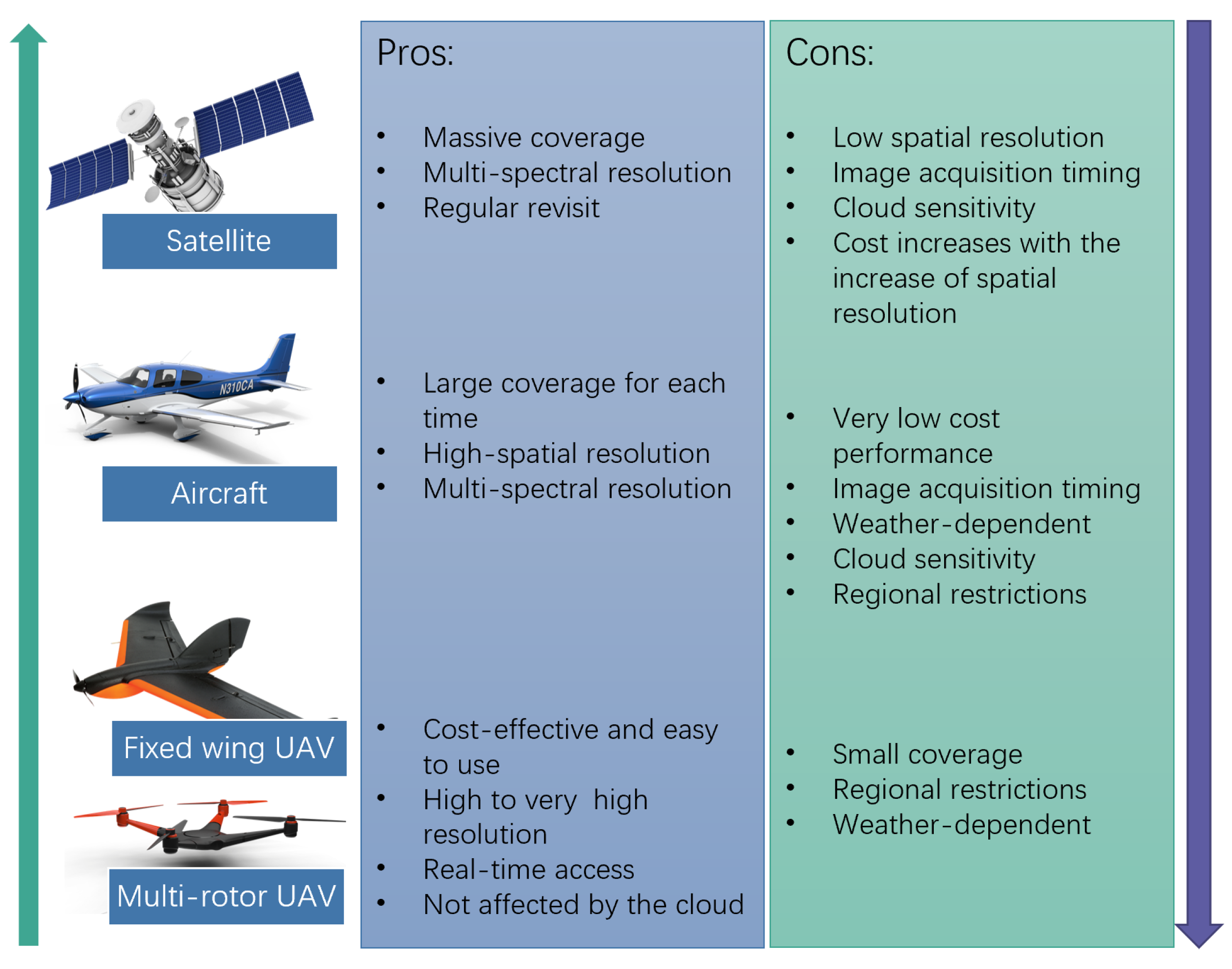
Figure 1. Pros and cons of the existing remote-sensing technologies.
Remotesensing 12 00417 g001
Figure 2. Architectures of three semantic segmentation classification models: (a) SegNet, (b) U-Net, (c) PSPNet.
Remotesensing 12 00417 g002
Figure 3. The architectures of four deep-learning-based object detection models: (a) Faster R-CNN and (b) cascade R-CNN are multi-stage detection models with two or more RPN modules; (c) SSD and (d) RetinaNet are single-stage detection models.
Remotesensing 12 00417 g003
Figure 4. The study area, Wushan county; the right figure shows the five data bands from visible (RGB) to near infrared (Nir) and the land cover labels used for model training.
Remotesensing 12 00417 g004
Figure 5. Sliding window method used for data preprocessing: 512 × 512 pixel moving window slides through the image with a setting distance (half of the sample size) each time to get a sample.
Remotesensing 12 00417 g005
Figure 6. Training images’ augmentation result after rotating, flipping, and mirroring.
Remotesensing 12 00417 g006
Figure 7. F1 score for each method across categories.
Remotesensing 12 00417 g007
Figure 8. Confusion matrices of the classification results achieved by the Segnet, U-net, PspNet, and merged methods based on the validation dataset.
Remotesensing 12 00417 g008
Figure 9. Wind turbine distribution in Inner Mongolia. The red box is the labelled bounding box for wind turbines, and the green points present the wind turbines’ locations on the map.
Remotesensing 12 00417 g009
Figure 10. Aggregated polygons on the initial result. The overlapping and closed objects were merged.
Remotesensing 12 00417 g010
Figure 11. Typical object detection results. Green box means the right detection results; otherwise, the red box shows the wrong results.
Remotesensing 12 00417 g011
Figure 12. The relationship between wind power generation in 2018 and the statistical number of wind turbines detected in seven provinces in China.
Remotesensing 12 00417 g012
Figure 13. The schematic diagram of the convolution and pooling layers.
Remotesensing 12 00417 g013
Figure 14. The spectral information of all categories.
Remotesensing 12 00417 g014
Figure 15. A comparison of random forest and the ensemble average of SegNet, U-Net, and PSPNet on land cover classification. The first column shows the RGB image, the second column shows the ground truth label, the third column shows the classification results from random forest, and the fourth column shows the classification results from the ensemble average of SegNet, U-Net, and PSPNet models.
Remotesensing 12 00417 g015
Figure 16. Typical results of a traditional multi-resolution segmentation method and two deep-learning- based semantic segmentation methods used in this study.
Remotesensing 12 00417 g016
Table 1. A comparison of average precision (AP) and inference speed of four different models. The bold numbers denote the optimal values in each column.
Model TypeModel NameBackboneAPAP after *Inf Speed (fps)
Multi-stageFaster R-CNNResnet500.9007530.98614224.6
Cascade R-CNN0.9035490.98830720.7
Single-stageSSD0.9034710.98745929.5
RetinaNet0.9034420.98548727.2
* AP after means the AP after polygon aggregation.
Table 2. The parameters of each semantic segmentation method learned in this work.
SegNetU-NetPSPNet
Input512 × 512 × 7512 × 512 × 7512 × 512 × 7
Layer94103293
Total params29,461,73634,615,75251,818,112
Trainable params29,445,84834,601,73651,759,872