Abstract
Hydrological models are usually calibrated against observed streamflow (Qobs), which is not applicable for ungauged river basins. A few studies have exploited remotely sensed evapotranspiration (ETRS) for model calibration but their effectiveness on streamflow simulation remains uncertain. This paper investigates the use of ETRS in the hydrological calibration of a widely used land surface model coupled with a source–sink routing scheme and global optimization algorithm for 28 natural river basins. A baseline simulation is a setup based on the latest model developments and inputs. Sensitive parameters are determined for Qobs and ETRS-based model calibrations, respectively, through comprehensive sensitivity tests. The ETRS-based model calibration results in a mean Kling–Gupta Efficiency (KGE) value of 0.54 for streamflow simulation; 61% of the river basins have KGE > 0.5 in the validation period, which is consistent with the calibration period and provides a significant improvement over the baseline. Compared to Qobs, the ETRS calibration produces better or similar streamflow simulations in 29% of the basins, while further significant improvements are achieved when either better ET or precipitation observations are used. Furthermore, the model results show better or similar performance in 68% of the basins and outperform the baseline simulations in 90% of the river basins using model parameters from the best ETRS calibration runs. This study confirms that with reasonable precipitation input, the ETRS-based spatially distributed calibration can efficiently tune parameters for better ET and streamflow simulations. The application of ETRS for global scale hydrological model calibration promises even better streamflow accuracy as the satellite-based ETRS observations continue to improve.
1. Introduction
Physically-based hydrological models are an essential tool for water resources planning, drought, and flood prediction, climate change assessment, and many other precipitation-runoff related applications. To achieve optimized performance, hydrological models are often calibrated against streamflow observations (hereafter termed Qobs), which measure integrated runoff fluxes [1,2,3]. However, Qobs may not always be the best applicable option for hydrological model calibration in various circumstances. Firstly, streamflow prediction in ungauged basins often uses the regionalization approach which transfers hydrological parameters from Qobs-based calibrations developed from donor gauged basins. Such regionalization methods tend to lose efficiency during the transfer process because the assumptions of spatial proximity and physical similarity are not always valid [4,5,6] Secondly, Qobs-based calibration has long been criticized for its equifinality problem, i.e., different parameter sets can satisfy the objective functions during the calibration period, while the model performance deteriorates significantly in the validation period [7,8]. Thirdly, Qobs calibration models tend to derive spatially homogeneous parameters across the river basin which neglects characteristic landscape heterogeneity [9]. Furthermore, to accomplish the “goodness-of-fit” between simulated and observed streamflow, Qobs calibration models are computationally time-consuming in routing spatially distributed runoff through complex drainage networks to produce estimated streamflow at the river basin outlet for each model time step [10].
Research has been conducted to calibrate hydrological models using observations of other water balance variables, such as soil moisture and evapotranspiration (ET) with or without observed streamflow [2]. Satellite-based estimations of these water balance variables have demonstrated value in providing spatially distributed observations with large geographical coverage at regular time intervals and with sufficient record length. For example, several remotely sensed ET records (hereafter referred to as ETRS) have been developed in recent years which differ in their governing equations, forcing data, and spatial and temporal scales of operation [11,12,13,14,15]. Many studies on the use of ETRS for hydrological model calibration have also been conducted ([16,17,18,19,20,21,22,23,24,25,26,27,28,29,30,31,32,33,34], see Table 1). As one of the pioneering studies in this field, Immerzeel and Droogers [16] optimized the parameters of the Soil and Water Assessment Tool (SWAT) model by tuning the modeled ET against ETRS for a human-regulated catchment in India. Their results showed close correspondence between the calibrated model ET and ETRS, although they were not able to provide direct validation of the model streamflow simulations due to heavy human-regulation of the study area. Subsequent studies modified the calibration approach by taking Qobs or ETRS as the calibration target independently using a single objective function or calibrating against both “Qobs + ETRS” simultaneously using a multi-objective function. Most of these studies concluded that, compared to the Qobs calibration scheme, the “Qobs + ETRS” calibration was able to improve the ET simulation while maintaining suitable model streamflow performance [18,19,20,21,24,25,26,28,29,30,31]. However, compared to the Qobs calibration model, some recent ETRS calibration models seem to result in a significant reduction in streamflow simulation accuracy [19,20,24,25], while the improvement of streamflow prediction skill is very low [21,22,26].

Table 1.
Literature reviews on integrating ETRS in hydrological model calibration. In the “ETRS*” column, either available ETRS products or user calculated ET using a specific equation with remote sensing data input are shown. In the “Model Configuration” column, the number of parameters involved in the calibration process is also included in the bracket for each study. The study of Nijzink et al. [27] employed five different conceptual models with multiple parameters; readers are recommended to investigate the original literature if interested; we used (*) to represent this complex case in the “Model Configuration” column.
As a critical hydrological component, ET represents moisture lost to the atmosphere from plants and soil, and thus significantly impacts the precipitation partitioning into different water balance components, particularly for runoff estimation. Hence, hydrological model performance should benefit from better ET accuracy by calibrating model parameters against high-quality ET observations. Previous studies using the ETRS calibration method have generally not demonstrated corresponding improvements in streamflow prediction performance. The lack of progress in this area reflects the need for a systematic investigation of the effectiveness of ETRS calibration and greater attention to the uncertainties in model inputs and model structure. The uncertainties in the ETRS estimations over space and time will directly influence the efficiency of the ETRS calibration method. Error in the input data, limitation of the algorithm in representing biophysical processes, and the uncertainty of biophysical and environmental parameters will together contribute to the biases in the ETRS estimations. When precipitation uncertainty is unknown or significant for hydrological model calibration [17,22,23,27,29,35], the optimization algorithm will be forced to adjust ET to compensate for errors in the precipitation inputs, rather than reducing parametric uncertainty. The lumped or oversimplified representation of hydrological processes and storages may be the main reason for poor streamflow performance [18,19,20,27]. The model structure limitation can cause serious difficulties in the attribution of the model performance to the ETRS calibration method, particularly in study areas with significant anthropogenic activities [16,17]. Furthermore, most prior studies have focused on only one small catchment, with the representativeness and transferability of the ETRS calibration results remaining unknown [23,24,25,30].
Given the significant improvement in ETRS estimation accuracy [36,37] and foreseeably higher-quality global ET products to be available in the near future, the ETRS calibration method may provide a viable approach for large scale or global hydrological modeling. For example, the need for better calibration is one of the major challenges of large scale hydrological modeling for global flood and drought prediction [38,39,40,41]. Therefore, the purpose of this study is to investigate the utility of remote sensing-based ET estimation in hydrological model calibration, emphasizing the evaluation of ETRS calibration impacts on streamflow simulation.
The following sections describe the methodology for this study, including the detailed calibration experimental design and a brief introduction of the hydrological model (Section 2); a description of the study area and datasets used (Section 3); a presentation of the major results (Section 4); followed by the conclusions of the implications of this work (Section 5).
2. Methodology
Previous studies involving ETRS calibration for hydrological modeling have largely adopted a lumped calibration method, whereby the modeled basin average ET is tuned toward spatially averaged ETRS observations. Relatively few studies have used the spatially distributed ETRS calibration method with all grid cells or sub-basins being treated individually [30,32,33]. The lumped ETRS calibration method relies heavily on the seasonal pattern of ETRS observations. The ETRS based spatially distributed calibration takes a further step than the lumped calibration by deriving an optimized spatially distributed model parameter set that accounts for the ETRS spatial patterns [9]. It is technically convenient to implement parallel computing for spatially distributed ETRS calibration on a per grid cell basis to reduce the computational load. For global applications and ungauged basins, this study tests the efficiency and effectiveness of the spatial ETRS calibration method based on the large-scale, semi-distributed, Variable Infiltration Capacity (VIC) model [42], coupled with a dominant river-tracing-based source-sink hydrologic routing scheme [43]. A total of 28 natural river basins (with negligible human interference) across a diversity of hydroclimate in the Pacific Northwest region are selected. The model simulations start on 1 January 1999, and end on 31 December 2013. The years 2004–2008 are used as the calibration period, while the 2009–2013 period is used for validation.
2.1. Hydrological Model
The VIC is a semi-distributed, physically-based hydrological model, and has been extensively used in studies involving water resources management, land-atmosphere interactions, and climate change [3,35,40,44,45,46,47,48,49,50]. A key challenge in the application of the VIC model in many large-scale applications has involved the need for automated calibration. Therefore, the VIC model has been tested, improved, and optimized for many regional river basins, resulting in relatively less uncertainty in various model inputs and predictions. Wu et al. [3] developed dominant river-tracing-based streamflow and temperature model, integrated with the VIC model, and successfully produced streamflow and temperature predictions at 1/16 degree resolution for the Pacific Northwest (PNW) domain. Here, we implement a similar modeling framework as Wu et al. [3], including the same VIC model components for ET and runoff simulations, the runoff-routing model, and calibration algorithms. The VIC model balances both the water and energy fluxes at the grid cell scale at each time step. While a sub-daily time step water-and-energy balance simulation is crucial in land-atmosphere studies, satisfying surface energy budgets requires substantial computational time, but has little influence on streamflow or ET simulations [51]. Therefore, we chose the VIC model running in the water balance mode at a daily time step for this study, similar to Wu et al. [3].
Based on Wu et al. [3], we set the VIC model run at 1/16-degree spatial resolution with subgrid spatial variability in vegetation and soil [48]. Vegetation parameters profoundly affect all components of the water cycle in the VIC model. The predefined subgrid vegetation parameters (e.g., land cover types, root depths) are set generally identical to those in previous studies [3,48,52], which were derived from the 1-km-resolution University of Maryland land cover database [53]. The subgrid soil parameters (e.g., bulk density, field capacity) are obtained from previous studies [3,48,52], which were derived from the 1-km-resolution Pennsylvania State University database [54]. The VIC model calibration processes for the streamflow simulation involves six parameters (Table 2). A primary effort of calibrating the VIC model for the major river basins over the Continental United States at the 1/8 degree resolution was made by Maurer et al. [48] by matching the simulated streamflow to available observations. The resulting parameters were used in the study of Wu et al. [3] for the Columbia River Basin. Livneh et al. [52] further refined the parameters B, Dsmax, and D3 at the 1/16-degree resolution using a similar method as Troy et al. [1] from which the resulting parameter set is taken as the baseline soil information input for this study.
Table 2.
The six soil parameters calibrated for the Variable Infiltration Capacity (VIC) model simulations in this study.
2.2. Model Calibration Experiments
A four-step workflow (Figure 1) was developed to perform the ETRS based spatially distributed calibration in this study and evaluate the impact of the ETRS calibration on the VIC model streamflow simulations. Major uncertainties for the model streamflow simulations are contributed from the model inputs (e.g., vegetation, soil, and precipitation inputs) and the simplified model structure that generally underrepresents the complexity of human-regulated river basins. Only upstream or headwater river basins without dams are selected for this study to emphasize natural flow conditions while minimizing model uncertainty impacts from river regulation.
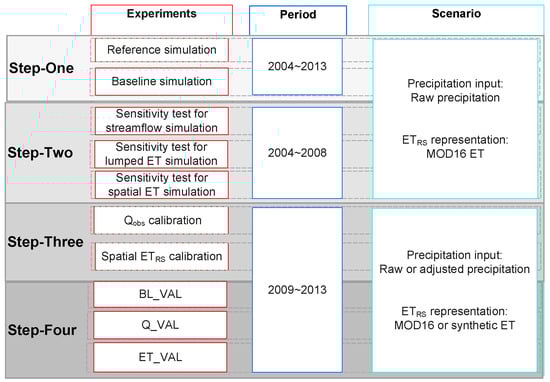
Figure 1.
The four-step scheme used to improve VIC model performance. In Step-One, reference and baseline simulations are performed to quantitatively evaluate the impact of different LAI inputs (Default LAI and Updated LAI) on modeled streamflow. In Step-Two, parameter sensitivity analysis tests for streamflow and ET are conducted to identify the most significant parameters in the calibration process. In Step-Three, the VIC model is calibrated against Qobs and the spatial ETRS target separately. In Step-Four, streamflow predictability skill is validated using baseline soil information (BL_VAL), soil information from Qobs (Q_VAL), and the spatial ET calibration model (ET_VAL). The uncertainties of precipitation and ETRS are considered in Step-Three and Step-Four, as listed in the Scenario column.
2.2.1. Updating Model Vegetation Inputs
We first evaluate and update the VIC model vegetation inputs using a satellite observation-based updated Leaf Area Index (LAI) dataset to define variations in canopy cover influencing the model ET calculations. Two widely used LAI climatology datasets are evaluated by comparing their corresponding streamflow prediction skills. The first LAI product is monthly averaged from a quarter-degree resolution monthly global LAI database [55] based on Advanced Very High-Resolution Radiometer (AVHRR) observations extending from 1981 to 1994. The AVHRR LAI record has been used for delineating vegetation cover in the VIC model in many prior studies [48,52] and is still widely used in VIC and other hydrological modeling applications [56,57,58,59,60,61,62]. The AVHRR LAI dataset is therefore referred to as the Default LAI record for this study. However, recent studies have found that temporally updated LAI inputs, rather than an outdated LAI monthly climatology, can improve VIC model performance [51,63,64,65]. Therefore, we adopted the 8-day, 1-km resolution GLASS/MODIS LAI record [66] as an additional model LAI input in this study, which extends over the 2004 to 2013 period and is monthly averaged as the Updated LAI record. The VIC model was then configured with the up-to-date vegetation information-based on the comparison of the streamflow simulations using the Default LAI and Updated LAI datasets.
2.2.2. Identifying Sensitive Parameters for Model Calibration
In the second step, we identified key model parameters influencing the resulting streamflow and spatial ET simulations. Given the up-to-date vegetation information used in the model, spatially distributed soil parameters are of critical importance. The model sensitivity tests are performed both at the river basin level and on a per grid cell basis, by separately varying each parameter equally over 100 intervals throughout the predefined parameter space (Table 2). This setting is useful for conducting a local sensitivity analysis, providing diagnostic insights on the model’s behavior around a point [67].
The Nash–Sutcliffe coefficient (NSC) [68] is used to evaluate the monthly streamflow simulation. The absolute Percent Bias (PBIAS) [69] is adopted to measure the 8-day spatial ET simulation and abbreviated as APBIAS hereafter.
where and are the monthly time series of streamflow observations and simulations respectively, and is the mean streamflow observation. and are the 8-day time series for the spatial ETRS observations and model ET simulations, respectively. The sensitivity index is then defined as the ratio between the difference and the sum of the maximum and minimum NSC (streamflow) per catchment or APBIAS (spatial ET) per grid cell among each parameter space setting (Equation (3)). A parameter is considered as more sensitive if the sensitivity index is closer to 1 than other parameters.
2.2.3. Calibration Model
In the third step, the spatial ETRS observations and Qobs calibration model are executed respectively using the Shuffled Complex Evolution (SCE-UA) global optimization method [70], which follows the modeling framework developed by Wu et al. [3]. The SCE-UA parameters (e.g., the number of complexes, the number of points in each complex) are recommended by [70] and 500 minimum iterations are set unless the parameters or objective function reach convergence prior to this threshold, within a ±1% level of further performance improvement. The objective functions of the Qobs and spatial ETRS calibration schemes are NSC (streamflow) and APBIAS (spatial ET), respectively.
The uncertainties in the ETRS and precipitation inputs were investigated; whereby, a synthetic ET calculation was derived from the simulation using the Qobs calibration optimized model parameters. A similar approach was used by [21] with favorable results. The synthetic ET results were then used for the spatially distributed model calibration, providing a reference to evaluate uncertainty contributed by the ETRS observations. A high-quality precipitation dataset is used in this study [52], and a simple correction approach is applied to further refine the precipitation product according to [35]. Specifically, annual reference precipitation at the basin scale is defined as the sum of the observed streamflow and ETRS for each hydrological year, assuming negligible annual soil water storage change for a water-budget closed river basin between hydrological years. The raw daily precipitation used in this study is then bias corrected by the annual reference precipitation. Such annual bias correction for precipitation input is proven to have positive impacts on streamflow simulations [35]. The further bias-corrected precipitation is then used to drive the model simulations for the comparison, and help understand the uncertainty contributed from the precipitation inputs.
2.2.4. Model Validation and Evaluation
In the fourth step, the effectiveness of the ETRS calibration on the streamflow simulation is evaluated by comparing the model results against independent observations, and through inter-comparison of outputs from different model experiments. Three model validation runs were performed for evaluating the Qobs calibration model (Q_VAL); spatial ETRS calibration model (ET_VAL); the baseline simulation model with the latest community efforts optimized soil information (BL_VAL).
The Kling–Gupta Efficiency (KGE) metric [71] was used to measure the agreement between observed and simulated monthly streamflow time series. The value of KGE ranges from negative infinity (no agreement) to one (perfect agreement).
where and are the mean and standard deviation of the streamflow observations; and are the mean and standard deviation of the streamflow simulations. We defined three general performance categories for the ET_VAL results, as improved (KGE improvement for streamflow > +10%) comparable (KGE improvement for streamflow within ± 10%), or degraded (KGE improvement for streamflow < −10% ) of their counterparts, respectively.
3. The Test Area and Datasets
The Columbia River Basin (CRB) encompasses approximately 668,000 km2 of the Pacific Northwest region of North America including portions of the Rocky Mountains in British Columbia, Canada. The CRB encompasses a wide range of physical and ecological environments ranging from semiarid and desert areas of the central plateaus to relatively wet forests in the Cascade Mountains [72]. The Columbia River drains the CRB and represents the fourth largest river in the continental United States. The water resources in the CRB have been extensively exploited in the past 70 years to meet various needs such as hydropower production, flood control, agricultural withdrawals, instream flow requirements for fish, and recreational needs [73].
River gauges in the CRB domain maintained by the U.S. Geological Survey (USGS) are selected for this study and used for model calibration and validation. Three general criteria were used for stream gauge selection, including (1) having continuous monthly discharge records from January 2004 to December 2013; (2) being identified as “reference gauges” (least-disturbed by human activities) in the Geospatial Attributes of Gages for Evaluating Streamflow (GAGES-II) database [74,75]; and (3) having dimensional consistency with the dominant river tracing (DRT) hydrography dataset defined at 1/16-degree spatial resolution [76]. The DRT river network upscaling algorithm, utilized 1-km-resolution HydroSHEDS (Hydrological data and maps based on SHuttle Elevation Derivatives at multiple Scales) baseline hydrography inputs, and successfully preserves critical sub-grid scale basin attributes affecting runoff and river flows [77,78]. To meet the requirements for criteria (3) above, the absolute relative difference between drainage areas derived from the DRT datasets and reported by the USGS has to be less than 20%, while visual inspection is also used to ensure geolocation accuracy. As a result, a total of 28 sub-basins in the CRB were selected for this study with sizes ranging from 325.70 km2 to 14,331.70 km2 (Figure 2). Detailed characteristics of the 28 basins can be found in Table 3.
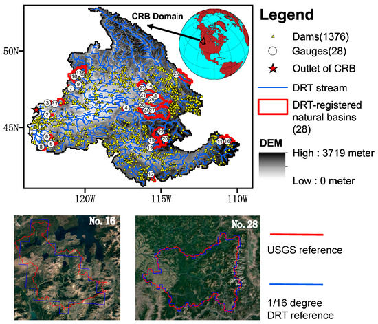
Figure 2.
The Columbia River Basin in the Pacific Northwest (PNW) of North America, which encompasses the 28 natural catchments examined in this study (numbered below). The DRT stream networks (1/16 degree spatial resolution) and the 28 DRT-registered unregulated catchments are overlaid on the HydroSHEDS DEM. River basin No.16 and No.28 plotted at the bottom of the figure are examples of the excellent co-geolocation between the DRT-registered upstream area and the USGS reference. The locations of major dams (yellow triangles) are obtained from the USGS National Hydrography Dataset.
Table 3.
Gauge information and basin characteristics of the 28 natural catchments examined in this study. Gauge information is retrieved from the USGS database, while basin characteristics are obtained from the GAGE-II database.
A recently updated gridded meteorological dataset for the Continental United States by Livneh et al. [52] is adopted for this study, which is an extended work of Maurer et al. [48] but has longer temporal coverage (1950 to 2013) and finer spatial resolution (1/16-degree). The quality-controlled dataset contains gridded precipitation, daily maximum and minimum temperature aggregated from point observations at National Weather Service Cooperative Observer (NWS COOP) stations, and surface winds from the National Centers for Environmental Prediction (NCEP)/ National Centers for Atmospheric Research (NCAR) reanalysis products. The gridded precipitation data are interpolated using the synergraphic mapping system (SYMAP) [79] and are scaled to match the Parameter-Elevation Regressions on Independent Slopes Model (PRISM) 1981–2010 precipitation climatology for topographic correction.
The widely used 8-day, 1-km resolution MODIS (MODerate resolution imaging spectroradiometer) MOD16 ETRS operational product [12] was used in this study. The MOD16 ET algorithm uses a modified Penman–Monteith algorithm driven by daily meteorological inputs from the NASA Global Modeling and Assimilation Office (GMAO) reanalysis, along with MODIS derived land cover, albedo, LAI, and enhanced vegetation index observations for global ET mapping and monitoring. The quality of the MOD16 ET record has been validated using tower eddy covariance-based daily ET measurements over North America [12,80,81,82]. Like other ETRS estimations, validation results of MOD16 products showed positive and negative bias in different places. Several studies have also used the MOD16 ET record for hydrological model calibration [20,27,30,31] and data assimilation [83]. For this investigation, the MOD16 ET record was geo-referenced and spatially aggregated to the 1/16-degree resolution PNW model grid.
4. Results
4.1. The Baseline Simulation
The hydrological model produced generally improved streamflow simulations in 68% (19 out of 28) of the test river basins when using the Updated LAI (mean KGE: 0.52) rather than the Default LAI (mean KGE: 0.45) as model inputs (Figure 3a). The differences in numerical streamflow modeling between the Default LAI and Updated LAI derived results can be large for some river basins. For river basin No.28, for example, Evergreen Needleleaf forest presents the highest LAI (Figure 3b,c), followed by Mixed Cover and Woodland vegetation types from both Default LAI and Updated LAI records. Significant discrepancies exist between the two LAI products, especially for the Evergreen Needleleaf class. The Default LAI fails to capture monthly variations in Evergreen Needleleaf forest, but generally captures similar monthly variations as the Updated LAI record for other land cover types, but with significant value differences, particularly for Mixed Cover. The LAI values are smaller and more spatially variable in the Updated LAI record than in the Default LAI for all the three major land cover classes, which is consistent with previous studies [84,85]. Lower LAI reduces transpiration from vegetation and evaporative losses from canopy interception, which promotes wetter soil conditions and greater surface and sub-surface runoff in the model [85].
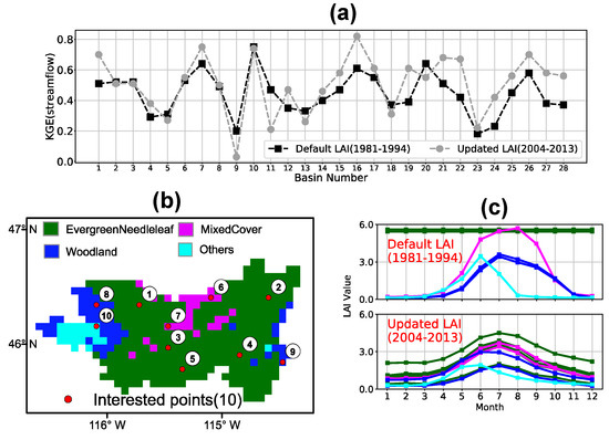
Figure 3.
Results of the reference and baseline simulations (Step-One). (a) Comparisons of streamflow simulation performances between Default and Updated LAI monthly climatology in the 28 catchments. (b) Land cover patterns for selected Basin No. 28; (c) monthly climatology between Default and Updated LAI for ten randomly selected locations within the basin (numbered in (b)) and representing different vegetation types distinguished by the same color scheme as (b).
Using a more temporally updated LAI record and more heterogeneous LAI data results in a marked improvement in the model streamflow predictions, as the seasonal LAI record is significant in the role of partitioning rainfall to runoff and ET in the VIC module. All of the following sections are based on model simulations using the Updated LAI record as a key input, allowing this study to build on recent advances in landscape parameterization.
4.2. Sensitivity Analysis of Soil Parameters
Model sensitivity tests were performed to identify the important parameters affecting both streamflow and the spatial ET simulations. Figure 4a suggests that all six of the soil parameters examined (Table 2) are essential for accurate streamflow simulations across all 28 study catchments, though the relative importance of the parameters varies across basins. However, the Ws and Ds parameters show the most significant individual influence on ET at the river basin scale (Figure 4b). The Dsmax and D3 parameters tend to have lower model sensitivity but are more effective than parameter D2. The model ET seems to show little sensitivity to parameter B in most of the test river basins.
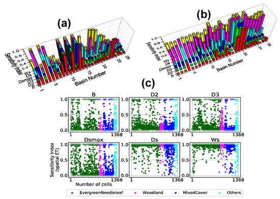
Figure 4.
Results of model sensitivity tests for streamflow and ET (Step-Two). (a) Sensitivity indices (Z-axis) of the six model soil parameters (Y-axis) adjusted for the streamflow simulation in each catchment (X-axis). (b) Sensitivity indices (Z-axis) of the six parameters (Y-axis) for the lumped ET simulation in each catchment (X-axis). (c) Sensitivity indices of the six parameters for the ET simulation of each grid cell classified by different land cover types.
Plots showing the sensitivity of the six model parameters at each individual grid cell in the four landscape groups are presented in Figure 4c; these results show the relative model sensitivity to the six parameters, which is consistent with the river basin scale results (Figure 4b). Most of the grid cell points are at the top of the Ws and Ds plots, indicating that the model ET calculations are highly sensitive to both parameters for all land cover classes (Figure 4c). The model is also sensitive to the other four parameters, but the sensitivity is more geolocation dependent. However, there were no significant differences in the model ET sensitivities to the model parameters among the four main landcover classes. However, the D2 parameter showed relatively less impact on the model ET calculation in woodlands due to the relatively thinner soil layer represented by this land cover class. Therefore, we allowed all six model parameters to vary in the Qobs calibration consistent with the majority of previous studies, while assuming B and D2 have no substantial impact on spatial ETRS calibration. Further research is warranted to investigate the validity of this assumption for other areas.
4.3. Uncertainty in the Calibrated Model Parameters
The model parameter ensembles paired with the NSC (streamflow) values from Qobs calibration are shown in Figure 5, six significant basins are selected to show the uncertainties in the calibrated model parameters against Qobs. For each of the six selected river basins, grey points denote all 500 evolutions in the Qobs calibration runtime; the 25 black points in each plot refer to equifinal simulations with NSC values very close to each other (within 1% difference), while the red point denotes the best streamflow prediction. The distribution of black points in the figure plots shows that Qobs calibration can yield very good streamflow predictions in most cases, with generally narrow ranges in the model parameter values. However, a lack of convergence in the calibrated parameters can be found in some river basins, indicating that “seemingly right” answers could be produced for the wrong reasons [30]. For example, at river basin No.16, all six model parameters except Ds, show large variations, indicating the low quality of model inputs (precipitation in particular), which may give the optimization algorithm more freedom to fit the objective function.
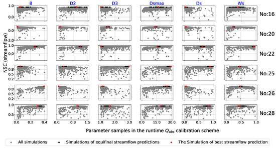
Figure 5.
The uncertainty associated with the parameters (X-axis) in the runtime Qobs calibration scheme and the propagation to streamflow simulations (Y-axis) (in Step-Three). For each basin, grey points are parameter ensembles for all iterations paired with the NSC (streamflow) in the runtime Qobs calibration scheme; black points refer to equifinal simulations, and the red point is the simulation of best streamflow prediction.
Keeping water balance closure can help ensure that a model with parameters constrained by reliable ETRS observations yields favorable runoff and streamflow predictions [17]. As shown in Figure 6, a number of river basins (e.g., No.2, 5, 7, 9, 10, 15, 16) show that improved ET prediction propagates to more accurate streamflow simulations. The model parameter set resulting in the best streamflow prediction (green star) is not (even close to) the one with the best ET simulation in many cases (except No. 15). This reflects both the limitations in the ETRS observations used for model ET calibration and the precipitation inputs. Effective spatial calibration of the parameter fields will be constrained as long as the errors in ETRS and the precipitation inputs remain larger than the variability in the calibrating parameters [32]. However, in all river basins, the model streamflow performance (i.e., KGE metrics) increases or decreases consistently with the gradient in ET bias. The calibration scheme steadily modulates the interplay of the errors in precipitation and ETRS, resulting in progressive changes of KGE values for streamflow simulation. For instance, if precipitation is biased high and ETRS biased low, a larger positive bias in ET would lead to a high KGE value for the streamflow simulation, while a successful ET calibration based on a relatively low biased ETRS would not necessarily produce a favorable streamflow simulation KGE result.
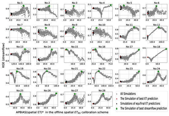
Figure 6.
The uncertainty associated with the parameters in the spatial ETRS calibration scheme and its propagation to streamflow simulations (in Step-Three). For each basin, the APBIAS (spatial ET)* (X-axis) is defined as the sum of the APBIAS (spatial ET) of all grid cells in each iteration, then sorted offline in ascending order (from smallest to largest bias between simulated ET and ETRS). The grey, black, and red points share similar references as Figure 5 but show spatial ET simulation performance. The green stars denote the locations of the best streamflow simulation performance.
As shown in Figure 6, when the ET and streamflow simulations simultaneously achieve good calibration performance (i.e., KGE for streamflow greater than 0.7), APBIAS for ET is less than 10% and the KGE value is very close to the best run (green star) result, which would also indicate good quality ETRS and precipitation inputs (e.g., the No. 15 river basin). On the other hand, if both the best run (green star) and corresponding streamflow simulation using the optimized model ET have a negative KGE value, the precipitation input may be considered as very low quality (see No.9 and 13). All of the rest (90%) of the test river basins in Figure 6 achieve positive KGE values with a mean of 0.50 for the model streamflow simulations after the ET calibration, indicating that the ETRS observations and precipitation inputs are of reasonable quality for most of the study basins. However, the distance between the actual (red point) and best run (green star) KGE results indicates potential room for further model improvements using better quality precipitation and/or ETRS records.
It is worth noting that incorporating the spatial distribution of the estimated parameters in the model calibration is a distinct advantage of the spatial ETRS calibration, which is considered a major challenge for large-domain hydrological modeling [9]. As shown in Figure 7, taking river basin No.28 as an example, the spatial ETRS optimized parameters show large spatial variability, while the Dsmax and Ds spatial distributions are similar and generally congruent with the pattern of soil texture (bulk density) across the catchment.
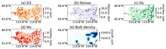
Figure 7.
The distributed soil parameters obtained from the spatial ETRS calibration model for selected Basin No.28 (in Step-Three) are depicted in (a–e) The “bulk density” from the defined soil information is used to represent soil texture.
4.4. Validation and Evaluation
As shown in Table 4, in the “Raw Precipitation” setup, KGE metrics from the validation simulations derived using model parameters from the ETRS calibration range from −0.11 to 0.95 (mean: 0.54). Approximately 61% of the study basins have KGE > 0.5, which is consistent with the calibration period results. Compared to the baseline validation, BL_VAL, in which the KGE values are between −0.12 and 0.85 (mean: 0.53).
Table 4.
The KGE metrics of streamflow predictability in BL_VAL, ET_VAL, and Q_VAL setups over the 28 study basins (involved in Step-Four). The basins No. 16, 20, 22, 25, 26, and 28 are illustrated in Figure 9 and highlighted below (in bold). The “MOD16 ET*” represents the optimum parameter set retrieved offline when observed and simulated streamflow fit best (green star in Figure 6).
The ET_VAL results show significant improvements in streamflow simulation, with 50% and 25% of the river basins showing improved and comparable performance, respectively. When compared to the Q_VAL, the ET_VAL results show improved and comparable performance for 18% and 11% of river basins, respectively, while 71% of the river basins show degraded performance (Figure 8a).
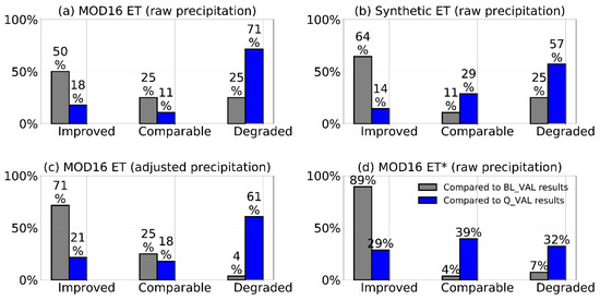
Figure 8.
Frequency histograms (cumulative percentage distributions over the 28 study basins) of ET_VAL efficiency in the categories of improved, comparable, and degraded) (in Step-Four). (a): Raw precipitation input is used to drive the calibration and validation schemes, and the ET_VAL uses the parameter set obtained when MOD16 ET and simulated ET fit to the global optimum (red points in Figure 6). (b) same as (a) but MOD16 ET is replaced by synthetic ET. (c) same as (a) but adjusted precipitation is used as the meteorological forcings of the model. (d) same as (a) but the optimum parameter set is retrieved offline when observed and simulated streamflow fit best (green star in Figure 6).
Using synthetic ET data for the model calibration causes significant improvements in model performance, with improved or comparable performance to BL_VAL for 64% and 11% of the study basins, respectively (Figure 8b). Thus, relatively closer model performance to Q_VAL is achieved using synthetic ET for the calibration, with a total of 43% of the river basins showing improved (14%) or comparable (29%) performance to Q_VAL. Using simply corrected precipitation in the ETRS calibration and validation, the streamflow simulations are also improved significantly over the ET_VAL results, with 39% of the study basins showing improved (21%) or comparable (18%) KGE metrics against Q_VAL (Figure 8c). Surprisingly, the simply corrected precipitation causes further marked improvement in the model performance, with 96% of the total river basins showing improved (71%) and comparable (25%) performance than the BL_VAL results. Further improvements in the model performance for both ET and streamflow simulations are also expected with better quality ET or precipitation inputs as shown in Figure 8b,c.
Furthermore, almost all the best model performances (in terms of streamflow) are achieved by using the parameter sets from the best KGE runs (i.e., green stars in Figure 6) using the ETRS calibration without involving streamflow observations. The best model runs represent 89% and 4% of the total study basins with improved and comparable performance to BL_VAL, respectively, and only 7% of the river basins with degraded metrics (Figure 8d). Interestingly, the ET_VAL results appear to be even better than the Q_VAL results, with 29% and 39% of the study basins showing improved and comparable KGE values, respectively. These results promote additional questions regarding how the best model runs can perform better than Q_VAL given the same maximum time of optimizing evolutions for the calibrations, and why the ETRS calibration approach can achieve very good streamflow simulations more efficiently than the Qobs calibration. Such improvements are likely due to the spatial distribution of ETRS, which may help the calibration scheme efficiently tune the model ET calculations at each grid cell toward optimal magnitudes, thereby improving the spatial distribution of runoff relative to the Qobs based model calibration. Understanding the internal processing structure to identify the best model run and optimal outputs under a diversity of climate and landscape conditions remains challenging and is warranted in future studies.
As shown in Figure 9, six river basins were selected to illustrate the ET_VAL simulated monthly hydrograph comparisons with Q_VAL, including two improved (No.20 and No.22), two comparable (No.16 and No.26), and two degraded (No.25 and No.28) basins from the adjusted precipitation setup (see Figure 8c). In the CRB domain, the snow melts in spring and accumulates in winter; thus, seasonal variations of modeled hydrograph are all well captured without consideration of parameter optimization method. For Basin No.20 and No.22 with improved performances of streamflow prediction, the ET_VAL results generally capture more flows than the Q_VAL results. For Basin No.16 and No.26 with comparable performances of streamflow prediction, the ET_VAL results for Basin No.16 overestimate flows in general and capture high flows well but fail in simulating low flow for Basin No.26. For both Basin No.25 and No.28 with degraded performances of streamflow prediction, ET_VAL underestimates high flows but overestimates low flows. All streamflow simulations do not capture the peak flows in the wet seasons of 2010 of all six basins. It is probable that the adjusted precipitation input here is insufficient to reflect discharge magnitudes.
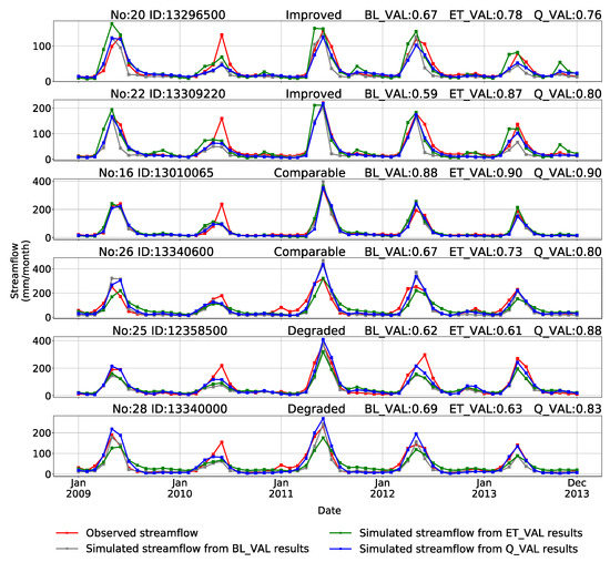
Figure 9.
Selected examples of simulated monthly streamflow derived from BL_VAL, ET_VAL, Q_VAL setups against monthly observed streamflow (involved in Step-Four). Of the six selected basins, two are improved (basin No.20 and No.22), two are comparable (basin No.16 and No.26), and two are degraded (basin No.25 and No.28) from the results obtained from the ET_VAL setup compared to the Q_VAL setup (see Figure 8c where adjusted precipitation setup is used). The X-axis is the monthly time series from 2009 to 2013; the Y-axis is the monthly observed and simulated streamflow.
5. Conclusions
In this study, we hypothesized that hydrological models calibrated against improved ETRS observations would lead to better streamflow predictions. A modeling framework developed by Wu et al. [3], including the widely used Variable Infiltration Capacity (VIC) model [42], the dominant river-tracing-based source-sink hydrologic routing model [43] and the SCE-UA global optimization algorithm [70] was adopted for model calibration, validation, and evaluation for 28 natural river basins in the Pacific Northwest region of the continental United States. The widely used MODIS MOD16 operational ET product [12] provided a spatially and temporally dynamic ET observational record (ETRS) for this study. A four-step workflow was designed to evaluate the impacts of the ETRS based spatially distributed model calibration for the streamflow simulations, and to clarify how the model parameters determine reasonable ET estimates coherent with other water budget components including precipitation, soil moisture, and runoff.
The baseline model simulations for this study used the latest VIC model inputs including precipitation, vegetation, and soil datasets. The resulting model simulations showed significant improvement in ET and streamflow simulations using a recently updated Leaf Area Index (LAI) climatology [66] as a critical input. Comprehensive model sensitivity tests were performed indicating a set of six critical model parameters for calibrating against Qobs, and four parameters for calibrating against ETRS (Table 2). Qobs based lumped calibration and ETRS based spatially distributed calibration were designed for this study, while uncertainties of precipitation and ET were considered to improve model performances (Figure 1). The validation results show that the model using the optimized parameters from the ETRS calibration results in a mean KGE value of 0.54, while 61% of the 28 natural river basins tested had KGE values exceeding 0.5. Importantly, the ETRS calibration scheme not only resulted in significant improvements over the baseline model, with 75% of the basins showing improved or comparable KGE metrics, but also resulted in consistent performance between model calibration and validation periods. Our results also indicate that either improved ET observations (indicated from a synthetic ET calibration experiment) or better precipitation inputs (through further bias correction) can provide further improvements to the effectiveness of the ET based calibration for better streamflow simulation. Compared to the Qobs calibration-based results, the synthetic ET based calibration produces better or comparable performance in 43% of the study basins, while the ETRS calibration using further annual bias-corrected precipitation produced better or comparable performance in 39% of the basins.
Interestingly, using the parameter sets from the best model calibration runs also produced the best overall model performance, with 93% and 68% of the study basins showing improved or close performance compared to the baseline simulations and the Qobs calibration-based results, respectively. Given reasonably accurate precipitation and ETRS records, the spatially distributed calibration scheme can be efficient in parameter optimization and effective in tuning the model for accurate streamflow calculations. However, if the precipitation inputs have a significant bias, the model calibration may still provide accurate streamflow simulations, but at the expense of degraded ET performance as the model ET parameters may be adversely adjusted to compensate for the bias in precipitation.
Our validation and evaluation results show that the ETRS calibration can efficiently tune the relevant model parameters for better ET and streamflow simulations within their physically meaningful ranges and with reasonable spatial distribution (e.g., consistent with soil texture patterns), which is likely due to the positive contribution from the spatial distribution information of ETRS. In gauged river basins with reliable Qobs data, the utility of ETRS in hydrological model calibration can further improve model performance by providing additional observational information to constrain the calibration. Moreover, our results demonstrate efficient and effective model calibrations using ET observations from global satellite records. These results are expected to be particularly beneficial for global-scale applications and natural basins lacking river gauge networks. The relative effectiveness of the model calibrations is expected to improve further as the quality of the ETRS observations continue to improve. A similar model calibration framework may apply to other satellite-based hydrological observations including soil moisture, surface inundation, snow cover, and river discharge. Further studies are needed to test the value of these observations for enabling further model calibration and performance enhancements.
Author Contributions
H.W. conceived the idea of the experiments, L.J. proposed the main structure of this study and performed the experiments; J.T. provided advice for the preparation of the original draft; J.S.K., L.A., and X.C. gave valuable advice on revising the manuscript. All authors have read and agreed to the published version of the manuscript.
Funding
This study was supported by National Natural Science Foundation of China (Grants 41775106, 41861144014, U1811464 and 41905101), the National Key R&D Program of China (grant no.2017YFA0604300), and also partially by Natural Science Foundation of Guangdong Province (grant no.2017A030313221) and the Program for Guangdong Introducing Innovative and Entrepreneurial Teams (No.2017ZT07X355). The authors also want to thank the anonymous reviewers for their constructive comments/suggestions.
Conflicts of Interest
The authors declare no conflict of interest.
References
- Troy, T.J.; Wood, E.F.; Sheffield, J. An efficient calibration method for continental-scale land surface modeling. Water Resour. Res. 2008, 44. [Google Scholar] [CrossRef]
- Arnold, J.G.; Youssef, M.A.; Yen, H.; White, M.J.; Sheshukov, A.Y.; Sadeghi, A.M.; Moriasi, D.N.; Steiner, J.L.; Amatya, D.M.; Skaggs, R.W.; et al. Hydrological processes and model representation: Impact of soft data on calibration. Trans. ASABE 2015, 58, 1637–1660. [Google Scholar] [CrossRef]
- Wu, H.; Kimball, J.S.; Elsner, M.M.; Mantua, N.; Adler, R.F.; Stanford, J. Projected climate change impacts on the hydrology and temperature of Pacific Northwest rivers. Water Resour. Res. 2012, 48. [Google Scholar] [CrossRef]
- Hrachowitz, M.; Savenije, H.H.G.; Blöschl, G.; McDonnell, J.J.; Sivapalan, M.; Pomeroy, J.W.; Arheimer, B.; Blume, T.; Clark, M.P.; Ehret, U.; et al. A decade of Predictions in Ungauged Basins (PUB)—A review. Hydrol. Sci. J. 2013, 58, 1198–1255. [Google Scholar] [CrossRef]
- Razavi, T.; Coulibaly, P. Streamflow prediction in ungauged basins: Review of regionalization methods. J. Hydrol. Eng. 2013, 18, 958–975. [Google Scholar] [CrossRef]
- Blöschl, G.; Sivapalan, M. Scale issues in hydrological modelling: A review. Hydrol. Process. 1995, 9, 251–290. [Google Scholar] [CrossRef]
- Beven, K.; Freer, J. Equifinality, data assimilation, and uncertainty estimation in mechanistic modelling of complex environmental systems using the GLUE methodology. J. Hydrol. 2001, 249, 11–29. [Google Scholar] [CrossRef]
- Beven, K. A manifesto for the equifinality thesis. J. Hydrol. 2006, 320, 18–36. [Google Scholar] [CrossRef]
- Mendiguren, G.; Koch, J.; Stisen, S. Spatial pattern evaluation of a calibrated national hydrological model—A remote-sensing-based diagnostic approach. Hydrol. Earth Syst. Sci. 2017, 21, 5987–6005. [Google Scholar] [CrossRef]
- Wi, S.; Yang, Y.C.E.; Steinschneider, S.; Khalil, A.; Brown, C.M. Calibration approaches for distributed hydrologic models in poorly gaged basins: Implication for streamflow projections under climate change. Hydrol. Earth Syst. Sci. 2015, 19, 857–876. [Google Scholar] [CrossRef]
- Glenn, E.P.; Neale, C.M.U.; Hunsaker, D.J.; Nagler, P.L. Vegetation index-based crop coefficients to estimate evapotranspiration by remote sensing in agricultural and natural ecosystems. Hydrol. Process. 2011, 25, 4050–4062. [Google Scholar] [CrossRef]
- Mu, Q.; Zhao, M.; Running, S.W. Improvements to a MODIS global terrestrial evapotranspiration algorithm. Remote Sens. Environ. 2011, 115, 1781–1800. [Google Scholar] [CrossRef]
- Anderson, M.C.; Allen, R.G.; Morse, A.; Kustas, W.P. Use of Landsat thermal imagery in monitoring evapotranspiration and managing water resources. Remote Sens. Environ. 2012, 122, 50–65. [Google Scholar] [CrossRef]
- Yan, H.; Wang, S.Q.; Billesbach, D.; Oechel, W.; Zhang, J.H.; Meyers, T.; Martin, T.A.; Matamala, R.; Baldocchi, D.; Bohrer, G.; et al. Global estimation of evapotranspiration using a leaf area index-based surface energy and water balance model. Remote Sens. Environ. 2012, 124, 581–595. [Google Scholar] [CrossRef]
- Yebra, M.; Van Dijk, A.; Leuning, R.; Huete, A.; Guerschman, J.P. Evaluation of optical remote sensing to estimate actual evapotranspiration and canopy conductance. Remote Sens. Environ. 2013, 129, 250–261. [Google Scholar] [CrossRef]
- Immerzeel, W.W.; Droogers, P. Calibration of a distributed hydrological model based on satellite evapotranspiration. J. Hydrol. 2008, 349, 411–424. [Google Scholar] [CrossRef]
- Winsemius, H.C.; Savenije, H.H.G.; Bastiaanssen, W.G.M. Constraining model parameters on remotely sensed evaporation: Justification for distribution in ungauged basins? Hydrol. Earth Syst. Sci. 2008, 12, 1403–1413. [Google Scholar] [CrossRef]
- Zhang, Y.; Chiew, F.H.S.; Zhang, L.; Li, H. Use of remotely sensed actual evapotranspiration to improve rainfall-runoff modeling in Southeast Australia. J. Hydrometeorol. 2009, 10, 969–980. [Google Scholar] [CrossRef]
- Rientjes, T.H.M.; Muthuwatta, L.P.; Bos, M.G.; Booij, M.J.; Bhatti, H.A. Multi-variable calibration of a semi-distributed hydrological model using streamflow data and satellite-based evapotranspiration. J. Hydrol. 2013, 505, 276–290. [Google Scholar] [CrossRef]
- Vervoort, R.W.; Miechels, S.F.; van Ogtrop, F.F.; Guillaume, J.H.A. Remotely sensed evapotranspiration to calibrate a lumped conceptual model: Pitfalls and opportunities. J. Hydrol. 2014, 519, 3223–3236. [Google Scholar] [CrossRef]
- Kunnath-Poovakka, A.; Ryu, D.; Renzullo, L.J.; George, B. The efficacy of calibrating hydrologic model using remotely sensed evapotranspiration and soil moisture for streamflow prediction. J. Hydrol. 2016, 535, 509–524. [Google Scholar] [CrossRef]
- López, P.L.; Sutanudjaja, E.H.; Schellekens, J.; Sterk, G.; Bierkens, M.F.P. Calibration of a large-scale hydrological model using satellite-based soil moisture and evapotranspiration products. Hydrol. Earth Syst. Sci. 2017, 21, 3125–3144. [Google Scholar] [CrossRef]
- Tobin, K.J.; Bennett, M.E. Constraining SWAT Calibration with Remotely Sensed Evapotranspiration Data. J. Am. Water Resour. Assoc. 2017, 53, 593–604. [Google Scholar] [CrossRef]
- Demirel, M.C.; Mai, J.; Mendiguren, G.; Koch, J.; Samaniego, L.; Stisen, S. Combining satellite data and appropriate objective functions for improved spatial pattern performance of a distributed hydrologic model. Hydrol. Earth Syst. Sci. 2018, 22, 1299–1315. [Google Scholar] [CrossRef]
- Herman, M.R.; Nejadhashemi, A.P.; Abouali, M.; Hernandez-Suarez, J.S.; Daneshvar, F.; Zhang, Z.; Anderson, M.C.; Sadeghi, A.M.; Hain, C.R.; Sharifi, A. Evaluating the role of evapotranspiration remote sensing data in improving hydrological modeling predictability. J. Hydrol. 2018, 556, 39–49. [Google Scholar] [CrossRef]
- Kunnath-Poovakka, A.; Ryu, D.; Renzullo, L.J.; George, B. Remotely sensed ET for streamflow modelling in catchments with contrasting flow characteristics: An attempt to improve efficiency. Stoch. Environ. Res. Risk Assess. 2018, 32, 1973–1992. [Google Scholar] [CrossRef]
- Nijzink, R.C.; Almeida, S.; Pechlivanidis, I.G.; Capell, R.; Gustafssons, D.; Arheimer, B.; Parajka, J.; Freer, J.; Han, D.; Wagener, T.; et al. Constraining Conceptual Hydrological Models with Multiple Information Sources. Water Resour. Res. 2018, 54, 8332–8362. [Google Scholar] [CrossRef]
- Pan, S.; Liu, L.; Bai, Z.; Xu, Y.P. Integration of remote sensing evapotranspiration into multi-objective calibration of distributed hydrology-soil-vegetation model (DHSVM) in a humid region of China. Water 2018, 10. [Google Scholar] [CrossRef]
- Poméon, T.; Diekkrüger, B.; Kumar, R. Computationally efficient multivariate calibration and validation of a grid-based hydrologic model in sparsely gauged West African river basins. Water 2018, 10. [Google Scholar] [CrossRef]
- Rajib, A.; Evenson, G.R.; Golden, H.E.; Lane, C.R. Hydrologic model predictability improves with spatially explicit calibration using remotely sensed evapotranspiration and biophysical parameters. J. Hydrol. 2018, 567, 668–683. [Google Scholar] [CrossRef] [PubMed]
- Wambura, F.J.; Dietrich, O.; Lischeid, G. Improving a distributed hydrological model using evapotranspiration-related boundary conditions as additional constraints in a data-scarce river basin. Hydrol. Process. 2018, 32, 759–775. [Google Scholar] [CrossRef]
- Becker, R.; Koppa, A.; Schulz, S.; Usman, M.; aus der Beek, T.; Schüth, C. Spatially distributed model calibration of a highly managed hydrological system using remote sensing-derived ET data. J. Hydrol. 2019, 577. [Google Scholar] [CrossRef]
- Odusanya, A.E.; Mehdi, B.; Schürz, C.; Oke, A.O.; Awokola, O.S.; Awomeso, J.A.; Adejuwon, J.O.; Schulz, K. Multi-site calibration and validation of SWAT with satellite-based evapotranspiration in a data-sparse catchment in southwestern Nigeria. Hydrol. Earth Syst. Sci. 2019, 23, 1113–1144. [Google Scholar] [CrossRef]
- Tobin, K.J.; Bennett, M.E. Improving alpine summertime streamflow simulations by the incorporation of evapotranspiration data. Water 2019, 11. [Google Scholar] [CrossRef]
- Wu, H.; Adler, R.; Tian, Y.; Gu, G.; Huffman, G. Evaluation of Quantitative Precipitation Estimations through Hydrological Modeling in IFloodS River Basins. J. Hydrometeorol. 2017, 18, 529–553. [Google Scholar] [CrossRef]
- Wang, K.; Dickinson, R.E. A review of global terrestrial evapotranspiration: Observation, modeling, climatology, and climatic variability. Rev. Geophys. 2012, 50. [Google Scholar] [CrossRef]
- Zhang, K.; Kimball, J.S.; Running, S.W. A review of remote sensing based actual evapotranspiration estimation. WIREs Water 2016, 3, 834–853. [Google Scholar] [CrossRef]
- Sheffield, J.; Wood, E.F.; Roderick, M.L. Little change in global drought over the past 60 years. Nature 2012, 491, 435–438. [Google Scholar] [CrossRef]
- Prudhomme, C.; Giuntoli, I.; Robinson, E.L.; Clark, D.B.; Arnell, N.W.; Dankers, R.; Fekete, B.M.; Franssen, W.; Gerten, D.; Gosling, S.N.; et al. Hydrological droughts in the 21st century, hotspots and uncertainties from a global multimodel ensemble experiment. Proc. Natl. Acad. Sci. USA 2014, 111, 3262–3267. [Google Scholar] [CrossRef]
- Wu, H.; Adler, R.F.; Tian, Y.; Huffman, G.J.; Li, H.; Wang, J. Real-time global flood estimation using satellite-based precipitation and a coupled land surface and routing model. Water Resour. Res. 2014, 50, 2693–2717. [Google Scholar] [CrossRef]
- Hirpa, F.A.; Salamon, P.; Beck, H.E.; Lorini, V.; Alfieri, L.; Zsoter, E.; Dadson, S.J. Calibration of the Global Flood Awareness System (GloFAS) using daily streamflow data. J. Hydrol. 2018, 566, 595–606. [Google Scholar] [CrossRef]
- Liang, X.; Lettenmaier, D.P.; Wood, E.F.; Burges, S.J. A simple hydrologically based model of land surface water and energy fluxes for general circulation models. J. Geophys. Res. 1994, 99, 14415–14428. [Google Scholar] [CrossRef]
- Olivera, F.; Famiglietti, J.; Asante, K. Global-scale flow routing using a source-to-sink algorithm. Water Resour. Res. 2000, 36, 2197–2207. [Google Scholar] [CrossRef]
- Xia, Y.; Mitchell, K.; Ek, M.; Sheffield, J.; Cosgrove, B.; Wood, E.; Luo, L.; Alonge, C.; Wei, H.; Meng, J.; et al. Continental-scale water and energy flux analysis and validation for the North American Land Data Assimilation System project phase 2 (NLDAS-2): 1. Intercomparison and application of model products. J. Geophys. Res. Atmos. 2012, 117. [Google Scholar] [CrossRef]
- Wood, A.W.; Leung, L.R.; Sridhar, V.; Lettenmaier, D.P. Hydrologic implications of dynamical and statistical approaches to downscaling climate model outputs. Clim. Change 2004, 62, 189–216. [Google Scholar] [CrossRef]
- Van Vliet, M.T.H.; Wiberg, D.; Leduc, S.; Riahi, K. Power-generation system vulnerability and adaptation to changes in climate and water resources. Nat. Clim. Change 2016, 6, 375–380. [Google Scholar] [CrossRef]
- Mote, P.W.; Hamlet, A.F.; Clark, M.P.; Lettenmaier, D.P. Declining mountain snowpack in western north America. Bull. Am. Meteorol. Soc. 2005, 86, 39–49. [Google Scholar] [CrossRef]
- Maurer, E.P.; Wood, A.W.; Adam, J.C.; Lettenmaier, D.P.; Nijssen, B. A long-term hydrologically based dataset of land surface fluxes and states for the conterminous United States. J. Clim. 2002, 15, 3237–3251. [Google Scholar] [CrossRef]
- Christensen, N.S.; Wood, A.W.; Voisin, N.; Lettenmaier, D.P.; Palmer, R.N. The effects of climate change on the hydrology and water resources of the Colorado River basin. Clim. Change 2004, 62, 337–363. [Google Scholar] [CrossRef]
- Barnett, T.P.; Pierce, D.W.; Hidalgo, H.G.; Bonfils, C.; Santer, B.D.; Das, T.; Bala, G.; Wood, A.W.; Nozawa, T.; Mirin, A.A.; et al. Human-induced changes in the hydrology of the Western United States. Science 2008, 319, 1080–1083. [Google Scholar] [CrossRef]
- Tang, Q.; Vivoni, E.R.; MuñOz-Arriola, F.; Lettenmaier, D.P. Predictability of evapotranspiration patterns using remotely sensed vegetation dynamics during the North American Monsoon. J. Hydrometeorol. 2012, 13, 103–121. [Google Scholar] [CrossRef]
- Livneh, B.; Bohn, T.J.; Pierce, D.W.; Munoz-Arriola, F.; Nijssen, B.; Vose, R.; Cayan, D.R.; Brekke, L. A spatially comprehensive, hydrometeorological data set for Mexico, the U.S., and Southern Canada 1950–2013. Sci. Data 2015, 2. [Google Scholar] [CrossRef] [PubMed]
- Hansen, M.C.; Sohlberg, R.; Defries, R.S.; Townshend, J.R.G. Global land cover classification at 1 km spatial resolution using a classification tree approach. Int. J. Remote Sens. 2000, 21, 1331–1364. [Google Scholar] [CrossRef]
- Miller, D.A.; White, R.A. A conterminous United States multilayer soil characteristics dataset for regional climate and hydrology modeling. Earth Interactions 1998, 2. [Google Scholar] [CrossRef]
- Myneni, R.B.; Ramakrishna, R.; Nemani, R.; Running, S.W. Estimation of global leaf area index and absorbed PAR using radiative transfer models. IEEE Trans. Geosci. Remote Sens. 1997, 35, 1380–1393. [Google Scholar] [CrossRef]
- Rajsekhar, D.; Mishra, A.K.; Singh, V.P. Regionalization of drought characteristics using an entropy approach. J. Hydrol. Eng. 2013, 18, 870–887. [Google Scholar] [CrossRef]
- Shukla, S.; McNally, A.; Husak, G.; Funk, C. A seasonal agricultural drought forecast system for food-insecure regions of East Africa. Hydrol. Earth Syst. Sci. 2014, 18, 3907–3921. [Google Scholar] [CrossRef]
- Lievens, H.; Al Bitar, A.; Verhoest, N.E.C.; Cabot, F.; de Lannoy, G.J.M.; Drusch, M.; Dumedah, G.; Hendricks Franssen, H.J.; Kerr, Y.; Tomer, S.K.; et al. Optimization of a radiative transfer forward operator for simulating SMOS brightness temperatures over the upper Mississippi basin. J. Hydrometeorol. 2015, 16, 1109–1134. [Google Scholar] [CrossRef]
- Rajsekhar, D.; Singh, V.P.; Mishra, A.K. Hydrologic drought atlas for Texas. J. Hydrol. Eng. 2015, 20. [Google Scholar] [CrossRef]
- Naz, B.S.; Kao, S.C.; Ashfaq, M.; Rastogi, D.; Mei, R.; Bowling, L.C. Regional hydrologic response to climate change in the conterminous United States using high-resolution hydroclimate simulations. Glob. Planet. Chang. 2016, 143, 100–117. [Google Scholar] [CrossRef]
- McNally, A.; Arsenault, K.; Kumar, S.; Shukla, S.; Peterson, P.; Wang, S.; Funk, C.; Peters-Lidard, C.D.; Verdin, J.P. A land data assimilation system for sub-Saharan Africa food and water security applications. Sci. Data 2017, 4. [Google Scholar] [CrossRef] [PubMed]
- Park, D.; Markus, M. A new method for establishing hydrologic fidelity of snow depth measurements based on snowmelt–runoff hydrographs. Hydrol. Sci. J. 2018, 63, 369–385. [Google Scholar] [CrossRef]
- Ford, T.W.; Quiring, S.M. Influence of MODIS-derived dynamic vegetation on VIC-simulated soil moisture in oklahoma. J. Hydrometeorol. 2013, 14, 1910–1921. [Google Scholar] [CrossRef]
- Parr, D.; Wang, G.; Bjerklie, D. Integrating remote sensing data on evapotranspiration and leaf area index with hydrological modeling: Impacts on model performance and future predictions. J. Hydrometeorol. 2015, 16, 2086–2100. [Google Scholar] [CrossRef]
- Bohn, T.J.; Vivoni, E.R. Process-based characterization of evapotranspiration sources over the North American monsoon region. Water Resour. Res. 2016, 52, 358–384. [Google Scholar] [CrossRef]
- Xiao, Z.; Liang, S.; Wang, J.; Chen, P.; Yin, X.; Zhang, L.; Song, J. Use of general regression neural networks for generating the GLASS leaf area index product from time-series MODIS surface reflectance. IEEE Trans. Geosci. Remote Sens. 2014, 52, 209–223. [Google Scholar] [CrossRef]
- Song, X.; Zhang, J.; Zhan, C.; Xuan, Y.; Ye, M.; Xu, C. Global sensitivity analysis in hydrological modeling: Review of concepts, methods, theoretical framework, and applications. J. Hydrol. 2015, 523, 739–757. [Google Scholar] [CrossRef]
- Nash, J.E.; Sutcliffe, J.V. River flow forecasting through conceptual models part I—A discussion of principles. J. Hydrol. 1970, 10, 282–290. [Google Scholar] [CrossRef]
- Gupta, H.V.; Sorooshian, S.; Yapo, P.O. Status of automatic calibration for hydrologic models: Comparison with multilevel expert calibration. J. Hydrol. Eng. 1999, 4, 135–143. [Google Scholar] [CrossRef]
- Duan, Q.; Sorooshian, S.; Gupta, V.K. Optimal use of the SCE-UA global optimization method for calibrating watershed models. J. Hydrol. 1994, 158, 265–284. [Google Scholar] [CrossRef]
- Gupta, H.V.; Kling, H.; Yilmaz, K.K.; Martinez, G.F. Decomposition of the mean squared error and NSE performance criteria: Implications for improving hydrological modelling. J. Hydrol. 2009, 377, 80–91. [Google Scholar] [CrossRef]
- Beechie, T.; Imaki, H. Predicting natural channel patterns based on landscape and geomorphic controls in the Columbia River basin, USA. Water Resour. Res. 2014, 50, 39–57. [Google Scholar] [CrossRef]
- Rajagopalan, K.; Chinnayakanahalli, K.J.; Stockle, C.O.; Nelson, R.L.; Kruger, C.E.; Brady, M.P.; Malek, K.; Dinesh, S.T.; Barber, M.E.; Hamlet, A.F.; et al. Impacts of Near-Term Climate Change on Irrigation Demands and Crop Yields in the Columbia River Basin. Water Resour. Res. 2018, 54, 2152–2182. [Google Scholar] [CrossRef]
- Falcone, J.A. GAGES-II: Geospatial Attributes of Gages for Evaluating Streamflow; US Geological Survey, 2011.
- Falcone, J.A.; Carlisle, D.M.; Wolock, D.M.; Meador, M.R. GAGES: A stream gage database for evaluating natural and altered flow conditions in the conterminous United States: Ecological archives E091-045. Ecology 2010, 91, 621. [Google Scholar] [CrossRef]
- Wu, H.; Kimball, J.S.; Mantua, N.; Stanford, J. Automated upscaling of river networks for macroscale hydrological modeling. Water Resour. Res. 2011, 47. [Google Scholar] [CrossRef]
- Kauffeldt, A.; Halldin, S.; Rodhe, A.; Xu, C.Y.; Westerberg, I.K. Disinformative data in large-scale hydrological modelling. Hydrol. Earth Syst. Sci. 2013, 17, 2845–2857. [Google Scholar] [CrossRef]
- Bisselink, B.; Zambrano-Bigiarini, M.; Burek, P.; de Roo, A. Assessing the role of uncertain precipitation estimates on the robustness of hydrological model parameters under highly variable climate conditions. J. Hydrol. Reg. Stud. 2016, 8, 112–129. [Google Scholar] [CrossRef]
- Shepard, D.S. Computer mapping: The SYMAP interpolation algorithm. In Spatial Statistics and Models; Springer, 1984; pp. 133–145. [Google Scholar]
- Velpuri, N.M.; Senay, G.B.; Singh, R.K.; Bohms, S.; Verdin, J.P. A comprehensive evaluation of two MODIS evapotranspiration products over the conterminous United States: Using point and gridded FLUXNET and water balance ET. Remote Sens. Environ. 2013, 139, 35–49. [Google Scholar] [CrossRef]
- Peters-Lidard, C.D.; Kumar, S.V.; Mocko, D.M.; Tian, Y. Estimating evapotranspiration with land data assimilation systems. Hydrol. Process. 2011, 25, 3979–3992. [Google Scholar] [CrossRef]
- Kumar, S.V.; Zaitchik, B.F.; Peters-Lidard, C.D.; Rodell, M.; Reichle, R.; Li, B.; Jasinski, M.; Mocko, D.; Getirana, A.; De Lannoy, G.; et al. Assimilation of Gridded GRACE terrestrial water storage estimates in the North American land data assimilation system. J. Hydrometeorol. 2016, 17, 1951–1972. [Google Scholar] [CrossRef]
- Zou, L.; Zhan, C.; Xia, J.; Wang, T.; Gippel, C.J. Implementation of evapotranspiration data assimilation with catchment scale distributed hydrological model via an ensemble Kalman Filter. J. Hydrol. 2017, 549, 685–702. [Google Scholar] [CrossRef]
- Peng, J.; Dan, L.; Dong, W. Estimate of extended long-term LAI data set derived from AVHRR and MODIS based on the correlations between LAI and key variables of the climate system from 1982 to 2009. Int. J. Remote Sens. 2013, 34, 7761–7778. [Google Scholar] [CrossRef]
- Xu, M.; Liang, X.Z.; Samel, A.; Gao, W. MODIS consistent vegetation parameter specifications and their impacts on regional climate simulations. J. Clim. 2014, 27, 8578–8596. [Google Scholar] [CrossRef]


© 2020 by the authors. Licensee MDPI, Basel, Switzerland. This article is an open access article distributed under the terms and conditions of the Creative Commons Attribution (CC BY) license (http://creativecommons.org/licenses/by/4.0/).