Abstract
Airborne hyper-spectral imaging has been proven to be an efficient means to provide new insights for the retrieval of biophysical variables. However, quantitative estimates of unbiased information derived from airborne hyperspectral measurements primarily require a correction of the anisotropic scattering properties of the land surface depicted by the bidirectional reflectance distribution function (BRDF). Hitherto, angular BRDF correction methods rarely combined viewing-illumination geometry and topographic information to achieve a comprehensive understanding and quantification of the BRDF effects. This is in particular the case for forested areas, frequently underlaid by rugged topography. This paper describes a method to correct the BRDF effects of airborne hyperspectral imagery over forested areas overlying rugged topography, referred in the reminder of the paper as rugged topography-BRDF (RT-BRDF) correction. The local viewing and illumination geometry are calculated for each pixel based on the characteristics of the airborne scanner and the local topography, and these two variables are used to adapt the Ross-Thick-Maignan and Li-Transit-Reciprocal kernels in the case of rugged topography. The new BRDF model is fitted to the anisotropy of multi-line airborne hyperspectral data. The number of pixels is set at 35,000 in this study, based on a stratified random sampling method to ensure a comprehensive coverage of the viewing and illumination angles and to minimize the fitting error of the BRDF model for all bands. Based on multi-line airborne hyperspectral data acquired with the Chinese Academy of Forestry’s LiDAR, CCD, and Hyperspectral system (CAF-LiCHy) in the Pu’er region (China), the results applying the RT-BRDF correction are compared with results from current empirical (C, and sun-canopy-sensor (SCS) adds C (SCS+C)) and semi-physical (SCS) topographic correction methods. Both quantitative assessment and visual inspection indicate that RT-BRDF, C, and SCS+C correction methods all reduce the topographic effects. However, the RT-BRDF method appears more efficient in reducing the variability in reflectance of overlapping areas in multiple flight-lines, with the advantage of reducing the BRDF effects caused by the combination of wide field of view (FOV) airborne scanner, rugged topography, and varying solar illumination angle over long flight time. Specifically, the average decrease in coefficient of variation (CV) is 3% and 3.5% for coniferous forest and broadleaved forest, respectively. This improvement is particularly marked in the near infrared (NIR) region (i.e., >750 nm). This finding opens new possible applications of airborne hyperspectral surveys over large areas.
1. Introduction
Airborne hyperspectral remote sensing technology improved significantly during the past decades, permitting a wide range and increasing number of applications such as land-cover type classification, forest biodiversity assessment, and quantitative estimation of land surface parameters [1,2,3,4,5]. Airborne scanners equipped with a wide field of view (FOV) provide a sampling of the bidirectional reflectance distribution function (BRDF) for very high spatial resolution (VHR) imagery [6,7]. Multiple angular scans associated with various solar irradiance for the same survey, together with the rugged topography of the area, results in strong anisotropic scattering effects for the studied area even for the same land-cover type, which is represented by the BRDF [8,9,10,11,12,13,14]. BRDF features can either be treated as perturbing effects or as additional information, this depending on the targeted objectives and applications [15,16,17,18]. BRDF correction is advised when mosaicking multiple hyperspectral scenes of a region, resulting in a spectrally homogeneous analysis-ready mosaic [19,20]. It is worth mentioning that an angular normalization procedure is mandatory to reduce the confounding non-biophysical signals and to sustain the interpretation of the airborne imagery in respect to land surface properties. VHR airborne hyperspectral images acquired over a rugged topography requires disentanglement of soil, vegetation canopy, and relief BRDFs, which remains challenging [21,22,23]. The problem is even more complex with airborne data due to the strong influence of the local slope and aspect.
A correct understanding of the BRDF effects is crucial for reflectance-based quantitative remote sensing inversion models [24,25]. Previous studies developed various statistical correction methods to remove the BRDF effects from satellite and airborne images (e.g., [20,26,27,28,29]). However, since these methods are not based on physical mechanisms of reflected light, they cannot be universally applied. Physical-based BRDF corrections usually require more detailed surface characteristics like the canopy structure and the ratio of direct and diffuse radiation for each pixel in order to simulate the radiative transfer mechanisms. This can be a time consuming procedure, which clearly limits its large scale use [30,31,32,33], while it remains still a challenging approach for even VHR airborne hyperspectral imagery. In this paper, the BRDF-RT model presented is based on a semi-empirical kernel-driven BRDF approach (e.g., [34]) utilizing the Ross-Li-Reciprocal model employed for Moderate Resolution Imaging Spectroradiometer (MODIS) BRDF/Albedo product suite (e.g., [35,36,37,38]) to normalize the off-nadir viewing directional reflectance to nadir BRDF adjusted reflectance. The MODIS BRDF algorithm and its physical basis have demonstrated to be a robust method and it has been widely used for BRDF correction of satellite images, for example to map land-cover types at the global scale [39,40,41].
The kernel-driven BRDF approach offers a synthetic vision of the complex scattering mechanisms of land surfaces via the linear combination of an isotropic kernel, a geometric-optical kernel, and a volumetric kernel. Various geometric-optical kernels (e.g., Li-Sparse-Reciprocal, Li-Dense-Reciprocal, Li-Transit-Reciprocal) and volumetric kernels (e.g., Ross-Thick, Ross-Thin, Ross-Thick-Maignan) having different mathematical expressions were proposed to optimally correct the observed scene. The prevalent combination of kernels in the literature is Ross-Thick and Li-Sparse-Reciprocal which describes the scene with a thick vegetation layer for the canopy and a sparse horizontal distribution of the stems. Numerous studies have attempted to extend the applicability of the MODIS satellite-specific BRDF algorithm to airborne hyperspectral images (e.g., [7,31,42]). Found issues were that different spatial scales of the image result in different BRDF effects, which limits the general applicability of the MODIS BRDF algorithm [43,44]. Hyperspectral images acquired using wide FOV airborne scanners typically have high spatial and spectral resolution. At the opposite to moderate resolution satellite images, pixels of a VHR image composed of less heterogeneous thematically different land-cover types is not common [45,46] but more physically as the limited number of vegetation attributes [15] infers strong structure-induced mutual shadowing effects, with, in the case of forests, traditionally a high level of clumping [2]. This affects the geometric-optical canopy model initially assumed, as well as the volume scattering component depending on the scenes, i.e., the forest stand scale. Therefore, an approach similar to the MODIS BRDF algorithm could still be considered but the higher level of details of an aerial hyperspectral image requires attention to be paid towards which scale of the scene is observed for further interpretation kernel-driven BRDF parameters.
Another critical aspect to be taken into account is that most BRDF models for airborne imagery assume flat topography [19,22,25] and disregard the forest covered areas over rugged topography. Variations in topography, especially in forested areas, could significantly affect the reliability of the soil-vegetation BRDF retrieval [14,47]. In order to mitigate the effects due to changing viewing and illumination geometry, previous research [14,48,49] used the slope and aspect information derived from a digital elevation model (DEM) to develop kernel-driven BRDF correction methods for Landsat images over rugged topography. Other methods for topographic correction typically use semi-empirical approaches to correct for the incidence BRDF effects mostly in a land cover-independent way [50,51,52,53]. However, exclusively based on anisotropic datasets premeasured in a laboratory environment [54,55], limited research has attempted to correct the BRDF effects of VHR airborne hyperspectral images with rugged topography for both viewing-illumination geometry and topography effects. Previous studies confirmed the need for a high resolution DEM or a forest canopy surface model in order to quantitatively map spatial phenomena in the rugged terrain areas. Current airborne integrated sensor systems are capable of measuring both spectral and terrain information of a pixel simultaneously. Examples include the Carnegie Airborne Observatory system (CAO; [56]), the Airborne Observation Platform (AOP) of the National Ecological Observatory Network (NEON; [57]), NASA Goddard’s LiDAR, Hyperspectral and Thermal (G-LiHT; [58]), and the Chinese Academy of Forestry’s LiDAR, CCD and Hyperspectral system (CAF-LiCHy; [59]). In addition, recent studies explored the potential of integrated airborne LiDAR and hyperspectral data for vegetation classification and ecological applications integrating data from different platforms (e.g., [60,61,62,63,64]). Ultimately, the increasing accessibility to high resolution data sets provides the unique opportunity to improve our understanding of BRDF correction algorithms for airborne hyperspectral imagery.
This paper describes an improved kernel-driven algorithm for the correction of the BRDF effects in VHR airborne hyperspectral images acquired using a push-broom wide FOV airborne scanner over rugged topography, i.e., rugged topography-BRDF (RT-BRDF) algorithm. To do so, we calculate the local viewing and illumination geometry for each pixel based on the scanner FOV information and LiDAR-derived DEM data. We then propose a stratified random sampling method for single-band BRDF modeling, ultimately extended to all spectral bands. Finally, local viewing and illumination angles are introduced to the kernel functions, resulting in an improved kernel-driven BRDF correction method for the studied forested areas with rugged topography. To assess the performance of the proposed RT-BRDF method, multiple flight-lines hyperspectral imagery and LiDAR-derived DEM were obtained using the CAF-LiCHy system, with both visual inspection and quantitative assessment performed by comparison with the results obtained using other methods (i.e., C, sun-canopy-sensor (SCS), and SCS+C). In this paper, another objective is to analyze and physically explain the scattering component (i.e., isotropic, geometric and volume scattering components) variations with the different observing scales through the quantitative BRDF parameters issued by the airborne VHR hyperspectral image and MODIS.
2. Study Area and Materials
2.1. Study Area
The study area (approximate coordinates: 22°27′–23°06′N; 100°19′–101°27′E) is located near the city of Pu’er in the Yunnan province of China. This region is among the south subtropical monsoon climate zone, with an annual average temperature of 17.9 °C and approximately 1350 mm of precipitation per year. The vegetation in the region is dominated by Pinus kesiya var. langbianensis and Monsoon evergreen broadleaved tree species (e.g., Castanopsis echidnocarpa, Castanopsis hystrix, Schima wallichii, Betula alnoides Buch.-Ham. ex D. Don) [65]. The area surveyed for this study is characterized by mountainous topography, with altitude varying between 500 and 2200 m above sea level and an average slope of 27°.
2.2. Remote Sensing Data
The hyperspectral data were acquired, respectively, under cloud-free conditions on 04 April and 06 April 2014 using the CAF-LiCHy system [59] at a nominal flight altitude approximately of 1500 m above mean ground elevation. Figure 1 shows the position of the 10 flight-lines of 04 April 2014 flight (yellow) and the four flight-lines of 06 April 2014 flight (green). Each designed flight-line had an average overlap rate of 20% with the adjacent hyperspectral image tracks. Table 1 summarizes the operational parameters of the CAF-LiCHy system. In the 04 April 2014 flight, the acquisition time was between 9:41 and 12:16 local time (i.e., from 1:41 to 4:16 UTC, 24-hour clock). The solar zenith and azimuth angles for the time of the flight was in the (24.0°–53.6°) and (100.4°–133.1°) ranges, respectively. In the 06 April 2014 flight, the acquisition time was between 9:48 and 10:35 local time (i.e., from 1:48 to 2:35 UTC, 24-hour clock). The solar zenith and azimuth angles for the time of the flight was in the (42.0°–50.5°) and (100.8°–106.5°) ranges, respectively. In this paper, the data of 06 April 2014 flight were utilized to construct the RT-BRDF algorithm in Section 3 and the results analyzed in Section 4. Then we applied the approach to a larger area (04 April 2014 flight) to assess the repeatability of the RT-BRDF algorithm, with results shown in Section 4.6.
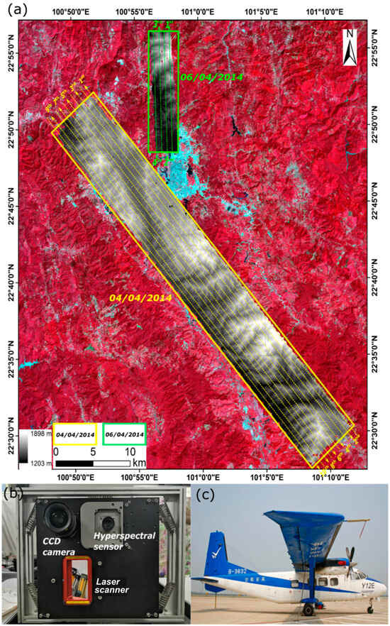
Figure 1.
(a) Location of the study area and schematic map of the 04 April 2014 (yellow) and 06 April 2014 (green) flight-lines overlying the 14 April 2014 false-color Landsat 8 OLI image (path/row = 130/044, bands 5, 4, 3) and airborne LiDAR-derived digital elevation model (DEM). (b) The CAF-LiCHy airborne system flown on the (c) Harbin Y-12E aircraft.

Table 1.
Parameters of the hyperspectral and LiDAR sensor of the CAF-LiCHy system.
The CAF-LiCHy system comprises an Airborne Imaging Spectrometer for Applications (AISA) Eagle II hyperspectral sensor (SPECIM Spectral Imaging Ltd., Oulu, Finland), an IGI DigiCAM-60 digital camera (Integrated Geospatial Innovations, Kreuztal, Germany), and a RIEGL LMS-Q680i Light Detection And Ranging (LiDAR) scanner (Riegl GmbH, Horn, Austria), providing hyperspectral images simultaneously with high resolution CCD images and LiDAR point cloud data [59]. The CCD images are orthorectified with 0.18 m spatial resolution.
The AISA Eagle II is a push broom imaging system with FOV of 37.7°. The hyperspectral images were obtained in 125/64 bands covering a spectral range spanning from 400 to 990 nm, with a spectral resolution of 4.6/9.2 nm. First, radiometric and geometric corrections of raw AISA Eagle II hyperspectral images were performed using CaligeoPRO v2.2.4 (SPECIM Limited, Oulu, Finland) which result in the radiance images with a ground sampling distance (GSD) of 1 m. Next, the hyperspectral images were atmospherically corrected using the ATCOR4 (ATmospheric CORrection 4) software (ReSe Applications LLC, Wil, Switzerland), to transform radiance into Bottom-Of-Atmosphere (BOA) apparent directional reflectance [7,66]. ATCOR4 calculates the database of atmospheric look-up table based on the MODTRAN5 (MODerate resolution atmospheric TRANsmission 5) code [67].
The LiDAR point cloud obtained has an average footprint density of 3 pts/m2. The LiDAR point cloud was separated into ground and non-ground return points data using the TerraScan software (Terrasolid, Helsinki, Finland) in order to generate a DEM and a digital surface model (DSM) with the resolution of 1 m. The DEM-derived slope and aspect were both calculated using a window size of 5 × 5 pixels in ENVI v5.3 (Exelis Visual Information Solutions, Boulder, CO, USA). The same GNSS and Inertial Navigation System (INS) module of the CAF-LiCHy leads to a high degree of geometric accuracy between the hyperspectral imagery and LiDAR-derived products.
To assess the performance of the RT-BRDF model for the VHR airborne hyperspectral images (AISA Eagle II hyperspectral data in this paper), the MODIS BRDF/Albedo Model Parameters and Nadir BRDF-Adjusted reflectance product (MCD43A1 and MCD43A4 Collection 6), corresponding to the flight date and location, were chosen for further comparison.
2.3. Field Data
A field survey was conducted from November 2013 to January 2014 in the study area to collect 61 circular sample plots with a radius of 15 m. A total of 30 plots were located in Pinus kesiya var. langbianensis dominated stands, and the remaining 31 plots in broadleaved forest stands. Within each plot, tree species, tree height, under-branch height, diameter at breast high (DBH), and crown diameter were measured for all the individual trees with DBH greater than 5 cm. Plot center location was recorded using a Trimble R4 Global Navigation Satellite Systems (GNSS) receiver (Trimble Navigation Limited, Sunnyvale, USA), with final post-differential processing position error resulting within 1 m.
3. Methodology
The procedure comprises the following three main steps: (i) calculate the rugged topography kernel functions based on local viewing and illumination geometry; (ii) calculate the kernel coefficients of the RT-BRDF model for each spectral band and each forest type; and (iii) apply the RT-BRDF model to correct for the anisotropy effects of airborne hyperspectral data. The detailed processing chain is described in Figure 2.
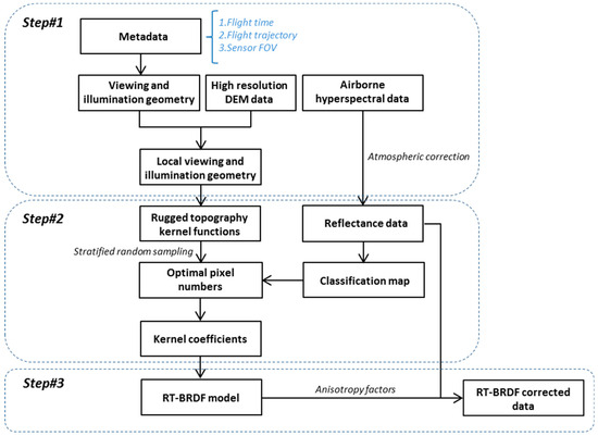
Figure 2.
Workflow of the rugged topography-bidirectional reflectance distribution function (RT-BRDF) correction method.
3.1. Land-Cover Stratification (Pre-Classification)
Different land-cover types present a priori different anisotropic properties. Therefore, a priori knowledge of the type is needed first to extract the BRDF characteristics pre land-cover type. Moreover, different canopy structure can impact the anisotropic properties even for forested areas. Studies in the literature (e.g., [68,69,70]) indicate that the texture information of VHR airborne optical images can represent a proxy to describe forest structure variables (e.g., crown diameter, tree height, tree density or spacing). For these reasons we applied a Support Vector Machine (SVM) classification method [71] to our hyperspectral images, using as input the BRDF cover index [7], the three most prominent components of the hyperspectral reflectance images obtained with the Principal Components Analysis method [72], and the Gray Level Co-occurrence Matrix (GLCM) texture features [73]. The GLCM texture features (i.e., mean, variance, homogeneity, contrast, dissimilarity, entropy, second moment, and correlation; [74]) are extracted based on the first principal component data with a window size of 9 × 9 pixels. In this study, coniferous forest, broadleaved forest, bare soil, urban, and unclassified were classified, with most unclassified pixels in our dataset represented by the cast-shaded areas in the deep gullies and canopy gaps [71].
3.2. Local Viewing and Illumination Geometry
In aerial hyperspectral imaging, each pixel has a different viewing and illumination geometry due to different scanning angles, imaging time, and topographic features. The relative sun-surface-sensor geometry is fundamental for the RT-BRDF method. In order to obtain this information, we developed a two-step process to calculate the local viewing and illumination geometry for each pixel of the airborne hyperspectral images, based on the characteristics of the wide FOV scanner utilized and the topographic features of the area surveyed, i.e., (i) calculate viewing and illumination geometry based on flat topography assumption; and (ii) transfer the viewing and illumination geometry to local viewing and illumination geometry based on a realistic topography issued from a high resolution DEM.
In the first step, the viewing and illumination geometries are calculated under the assumption of a flat topography. Since each flight-line is acquired in a relatively short period of time (i.e., approximately 10 min), the solar position within this time period is assumed to be constant here. Thus, both solar zenith and azimuth angles are calculated based on date, average latitude and longitude, and median acquisition time in each flight-line. For each pixel, the image space coordinates are converted into object space coordinates using the co-linearity equations in Equations (1) and (2) [75]:
where and represent the pixel vector in the object space coordinates and image space coordinates, respectively; is the rotation matrix calculated from the exterior orientation element , , and ; is the focal length of the optical camera; and is the principal point in image space coordinates.
View zenith and azimuth angles are calculated for each pixel using Equations (3) and (4):
where and are the view zenith and azimuth angle, respectively.
Due to the fact that the majority of the species in our study area grows vertically independently of the slope of the terrain, and in order to apply the Li-Strahler geometric-optical model to sloping terrain, the ellipsoidal tree crown is replaced by spheres casting the same shadow area. The slope is converted to the forest-adjusted slope (Equation (5)). In the second step, the global coordinates obtained as described in Equation (1) are transformed into local coordinates based on converted slope and aspect angle of each pixel (Equation (6); [76]):
where r/b represents the ratio of horizontal crown radius to vertical crown radius; is the pixel vector in local coordinates; and is the rotation matrix based on topographic features calculated from the converted slope and aspect angle of each pixel.
Then, real local view angles are calculated for each pixel using Equations (7) and (8). Similarly, real local solar zenith angle and solar azimuth angle can be calculated according to each pixel using Equation (6):
where and are the local view zenith and azimuth angle for each pixel, respectively.
Finally, the cosine of the local solar zenith angle can be referred as illumination conditions, and it is calculated as in Equation (9):
where and are the solar zenith angle and relative azimuth angle between the aspect and sun azimuth based on flat topography, respectively.
3.3. Rugged Topography BRDF Model and Kernel Selection
We assume that each land-cover type in the images presents a homogeneous structure and does not vary with the slope and aspect of the underlying topography (i.e., relatively uniform anisotropic properties). The local viewing and illumination geometry result in a multi-angular data set for each land-cover type [77]. A kernel-driven BRDF approach (e.g., [34]), used in literature from the canopy to the satellite scale (e.g., [24,78,79]), was adopted in this study. Specifically, this model is based on the linear combination of volumetric, geometric, and isotropic scattering effects. However, despite having similar fitting capability to the Li-Sparse kernel, the Li-Transit kernel has demonstrated to perform better in the case of high solar and/or view zenith angles [80]. Therefore, in this study the Li-Transit-Reciprocal (LTR) kernel [81,82] was used as geometric scattering kernel, and the hotspot-revised Ross-Thick-Maignan (RTM) kernel [83] as volumetric scattering kernel. Using the local viewing and illumination angles in the RTM and LTR kernel functions, the RT-BRDF model can be expressed as in Equation (10):
where:
where , , , , and are the local view zenith angle, local solar zenith angle, and local relative azimuth angle between the sun and the observer, land-cover type, and wavelength respectively; , , and are coefficients of isotropic scattering, volume scattering and geometric scattering, respectively; is the volume scattering kernel; and is the geometric scattering kernel. A constant value of is used to indicate the half-width of the hotspot for most of the targets [83]. The Li-Transit kernel requires to set the parameters for the tree crown geometry. In accordance with the field measurements, in this study we used h/b = 2 and b/r = 1 for coniferous forest; and h/b = 1.5 and b/r = 1 for broadleaved forest.
3.4. Determination of BRDF Model Coefficients
VHR airborne hyperspectral images generally contain a large number of pixels. For the purpose of an efficient processing and in order to obtain a comprehensive coverage of the viewing and illumination angles, a stratified random sampling method [84,85] was used to select a subset of pixels for the BRDF model fitting. For instance, under the assumption that the data set used in this study included a high number of pixels (N) in coniferous forest covered areas, a subset of n pixels were chosen from the N pixels (with n << N, with N ≈ 18,500,000 in this case) to build the BRDF model for coniferous forest in our study according to the following sampling rules (Figure 3):
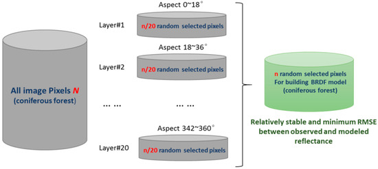
Figure 3.
Flowchart of the stratified random sampling method for coniferous forest pixel selection.
- n takes any values between 100 and 50,000, with step length of 100 pixels (i.e., 100, 200, 300, …, 49,900, 50,000);
- aspect values between 0° and 360° are divided into twenty 18° classes (i.e., 0°–18°, 18°–36°, …, 342°–360°);
- for each 18° class, n/20 coniferous pixels are chosen randomly;
- the root mean square errors (RMSE) between the observed band reflectance and the model fitted band reflectance is used to determine the optimal n (i.e., we define the optimal n here as the minimum n pixels with a relatively stable and minimum RMSE for the BRDF model fitting).
In order to obtain the optimal number of pixels for each spectral band (i.e., 125 bands, 400–990 nm), we developed an independent band normalized RMSE (Equation (22)) for each band:
where and indicate the minimum and maximum RMSE for the different set n pixels (i.e., from 100 to 50,000 in this study), respectively.
Once the optimal number of pixels n is determined for each class type, the kernel coefficients for each band can be determined using the least square method, which solution is shown in Equation (23):
in Equation (23), the , ,…, and , ,…, represent the volumetric and geometric scattering kernel for the 1st, 2nd,…,nth pixel, respectively; and , ,.., is the observed band reflectance for the 1st, 2nd,…, nth pixel. The Equation (23) can be written as a matrix form in Equation (24) and can be further expressed as a simplified form in Equation (25). Then the kernel coefficients can be calculated as .
3.5. BRDF Effects Correction for Image
The anisotropy factor (ANIF) is a ratio describing the relationship between directional reflectance and reference reflectance, and it is introduced to the BRDF correction model of the hyperspectral image. We followed the approach described in [31], and defined the ANIF with respect to the nadir reflectance as in Equation (26); therefore, the RT-BRDF corrected reflectance () can be calculated using Equation (27):
where is the simulated BOA apparent reflectance at nadir; and represent the fixed solar position; and is the ATCOR-corrected apparent directional reflectance as mentioned in Section 2.2.
3.6. RT-BRDF Performance Assessment
In order to evaluate the performance of the RT-BRDF method, three assessment strategies were used qualitatively and quantitatively [7,53,86,87], which included (a) comparisons of the results with other topographic correction approaches; (b) comparisons with the MODIS products; (c) utilizing the fitted RT-BRDF correction coefficient to another larger area for the robustness verification. The specific operations are as follows.
- (a)
- The results of three commonly used topographic correction approaches (i.e., C, SCS, and SCS+C, see Table 2) were compared to RT-BRDF. Specifically, we implemented the following goals:
Table 2. Topographic correction methods for RT-BRDF performance assessment.
- First, since an effective correction method can produce a highly homogeneous mosaic imagery without topographic and BRDF (solar-viewing geometry) effects, a visual inspection was performed focusing on the topographic correction results and the variability of the overlapped area of adjacent flight-line images.
- Previous studies [49,66,88] observed a positive linear relationship between surface reflectance and illumination conditions. An effective BRDF correction method can remove this relationship and result in the R2 and slope value of the linear function approaching zero.
- The terrain-induced canopy BRDF can lead to reflectance variations with slope and aspect (i.e., topographic conditions). Practically, sun-facing pixels would potentially have higher reflectance than pixels lying on shaded slopes. An effective BRDF correction method can weaken the influence of topographic conditions, resulting in a more homogeneous spectral balance between sunlit and shaded areas.
- Based on the assumption of homogeneous structure for each forest type, we followed the approach described in [87] focusing on the reflectance over the aspect of pixels perpendicular to the solar direction. An effective correction method can obtain a nearly perfect fit between uncorrected and corrected reflectance of these pixels.
- Finally, this mitigation effect can be further confirmed by the analysis of the RMSE of the reflectance variation in the forested pixels (i.e., coniferous and broadleaved forest) from overlapping pixels of two adjacent hyperspectral images. In fact, a further effect of the BRDF correction is to decrease the standard deviation of the reflectance spectra for each land-cover type [53]. The coefficient of variation (CV) defined in Equation (28) is utilized to evaluate the results obtained with the RT-BRDF method:
- (b)
- The weighting parameters of the MODIS BRDF/Albedo Model Parameters product were identified from the relatively pure forest pixels. Then we performed the comparison of the VHR pixel-based three BRDF model weighting parameters (, , and ) of AISA Eagle II bands (400–990 nm) with the coarse scale (500 m) weighting parameters of MODIS band1–4, respectively. Further, 500 × 500 AISA Eagle II pixels (500 × 500 m) were aggregated to match the MODIS pixel and to assess the difference of the nadir BRDF-adjusted forest reflectance between the aggregated AISA Eagle II data and MODIS data. Specifically, the AISA Eagle II band reflectance corresponding to the reflectance of MODIS band’s central wavelength (i.e., AISA Eagle II band54, 644.8 nm for MODIS band1, 620–670 nm; AISA Eagle II band98, 856.6 nm for MODIS band2, 841–876 nm; AISA Eagle II band16, 467.9 nm for MODIS band3, 459–479 nm; AISA Eagle II band35, 555.4 nm for MODIS band4, 545–565 nm).
- (c)
- In order to assess the repeatability of the algorithm, we applied the RT-BRDF method to a larger area (04 April 2014 flight campaign) to verify whether the BRDF effects of airborne hyperspectral imagery over forested areas with rugged topography can be corrected.
4. Results
4.1. Preprocessing Results
The training and test data for the forest type classification were obtained from field work (Section 2.3) and visual interpretation of high resolution CCD images. The overall classification accuracy and kappa coefficient of the airborne hyperspectral data are 94.9% and 0.93, respectively. Theoretical (i.e., flat topography hypothesis) and calculated viewing and illumination geometry from a selected region of the hyperspectral images are shown in Figure 4a–d and Figure 4e–h, respectively. When compared to the hypothetical case, the slope and aspect of the surveyed topography lead to a wider range of local viewing and illumination geometry and consequently a multi-angular observation data set for the same land-cover type.
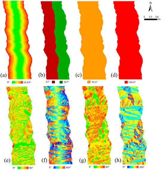
Figure 4.
Local viewing and illumination geometry for a hyperspectral sample extracted from the first (i.e., easternmost) flight-line (06/04/2014). (a)–(d) respectively show the theoretical view zenith angle (VZA), view azimuth angle (VAA), solar zenith angle (SZA), and solar azimuth angle (SAA) under the assumption of flat topography; (e)–(h) instead, respectively, show local VZA, local VAA, local SZA, and local SAA for the surveyed area.
4.2. Optimal Pixel Numbers for BRDF Modeling
In this study, the optimal number of pixels for the BRDF modeling is defined as the minimum number of pixels, and was selected using a stratified random sampling method, which is necessary to achieve minimum RMSE between observed and model simulated reflectance. The calculated RMSE for a reference near infrared (NIR) band (i.e., band 94, 837.19 nm) is shown in Figure 5a,b for coniferous and broadleaved forest, respectively. The results in Figure 5a,b show that the RMSE declines dramatically with the number of pixels increasing from 100 to 10,000, and especially below 1000. In contrast, the RMSE remains low with increasing number of pixels from 10,000 to 50,000, and especially greater than 35,000. For both coniferous and broadleaved forest, for each band, the independent band normalized RMSE with number of pixels from 100 to 50,000 is shown in Figure 5c,d. For band 94, the trend of RMSE (Figure 5a,b) can therefore be represented as a consistent trend of independent band normalized RMSE (Figure 5c,d). The independent band normalized RMSE show similar overall trends for the majority of bands and forest types: (i) a rapid decline of RMSE with number of pixels increasing from 100 to 10,000; (ii) stabilization with number of pixels greater around 10,000; and (iii) consistently low RMSE value (i.e., <0.001) with number of pixels greater than 35,000. Ultimately, in this study the number of pixels n is set at 35,000 to ensure a comprehensive coverage of the viewing and illumination angles and higher fitting accuracy of the BRDF model for all bands.
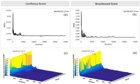
Figure 5.
Optimal number of selected pixels for BRDF model building of band 94 (837.19 nm). (a) and (b) show the root mean square error (RMSE) between observed and model simulated reflectance of coniferous and broadleaved forest, respectively; (c) and (d) respectively indicate the independent band normalized RMSE (corresponding to selected number of pixels n) for all the bands of coniferous and broadleaved forest, with independent band 94 normalized RMSE plotted in black.
4.3. BRDF Correction of Topographic Effect
Figure 6 shows a false-color composite (i.e., 837.19, 694.91, and 543.72 nm band for R, G, and B, respectively) close-up of the pre- (i.e., no terrain induced atmospheric effects corrected) and post-correction hyperspectral images. The overlaps between adjacent hyperspectral images and the final mosaic outline is displayed in Figure 6a. At a first visual inspection, it can be observed that the reflectance in the BRDF uncorrected mosaic (Figure 6b) is significantly affected by topographic effects (e.g., shaded pixels darker than illuminated pixels). However, it can be noticed that the RT-BRDF, C, and SCS+C correction method effectively reduce these topographic effects as shown in Figure 6c, Figure 6d,f, whereas the SCS correction in Figure 6e led to an obvious overcorrection in the weakly illuminated areas. Figure 6d,f also shows that both C and SCS+C corrected images still present a slight overcorrection in the backscattering regions (i.e., same observing direction and solar incidence direction [91] for each flight-line image). The full-sized RT-BRDF corrected and uncorrected images are displayed in the next with selected areas magnified to show significant differences (cfr. Figure 14).
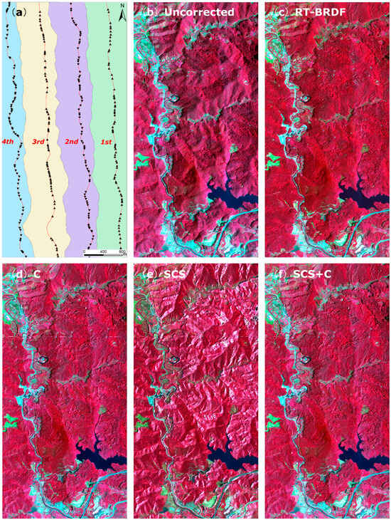
Figure 6.
Comparison between the pre-and post-corrected hyperspectral mosaics displayed as false-color composites (i.e., 837.19, 694.91, 543.72 nm band for the R, G, and B channels, respectively): (a) outline of hyperspectral flight-lines and mosaic; (b) pre-corrected (no terrain induced atmospheric effects corrected) mosaic; (c) RT-BRDF corrected mosaic; (d) C corrected mosaic; (e) Sun-canopy-sensor (SCS) corrected mosaic; (f) SCS+C corrected mosaic.
To quantitatively analyze the topographic correction effects under varying illumination conditions, the relationship between reflectance of a selected NIR band (i.e., 837.19 nm) and the cosine of the local solar incidence angle (i.e., illumination condition) is shown in Figure 7, where 500 non- shadowed pixels were randomly selected from the hyperspectral mosaic for both coniferous and broadleaved forest. Figure 7a,f show the relationship between illumination conditions and uncorrected reflectance at 837.19 nm for coniferous (R2 = 0.26) and broadleaved forest (R2 = 0.30). This moderate correlation is almost entirely removed by the RT-BRDF (R2 = 0.0014 and 0.000002, respectively; Figure 7b,g), the C correction (R2 = 0.0072 and 0.0014, respectively; Figure 7c,h), and the SCS+C correction (R2 = 0.0096 and 0.0038, respectively; Figure 7e,j). However, the SCS correction results in a stronger linear relationship between surface reflectance and illumination conditions for both coniferous and broadleaved forest (R2 = 0.34 and 0.54, respectively; Figure 7d,i), consistently with the visually overcorrected mosaic in Figure 6e. Similarly, compared to the RT-BRDF corrected mosaic, occurrences of slight overcorrection can also be noticed in both the C and SCS+C corrected mosaics (Figure 6d,f) for low illumination conditions (i.e., <0.2).
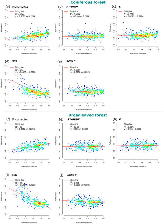
Figure 7.
Density scatterplots of the relationship between illumination conditions and reflectance at 837.19 nm for coniferous (a–e) and broadleaved (f–j) forest. (a) Uncorrected, (b) RT-BRDF, (c) C, (d) SCS, and (e) SCS+C corrected reflectance values of coniferous forest pixels; (f) uncorrected, (g) RT-BRDF, (h) C, (i) SCS, and (j) SCS+C corrected reflectance values of broadleaved forest pixels.
Figure 8 shows the variation of reflectance at 837.19 nm with slope and aspect (i.e., topographic conditions). Figure 8a,f show an overall higher uncorrected reflectance of the broadleaved forest pixels in a great majority of topographic conditions compared to the uncorrected reflectance of coniferous forest pixels. Consistently with the results in Figure 8a,f, sun-facing aspect classes (i.e., high illumination conditions) display higher uncorrected reflectance values for both forest types. Conversely, the RT-BRDF, C, and SCS+C corrected reflectance of both coniferous and broadleaved forest pixels show a significant reduction of this positive relationship with topographic conditions. However, the SCS correction resulted in higher reflectance values for the shaded aspect classes (i.e., overcorrection; Figure 8d,i).
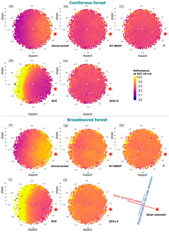
Figure 8.
Bottom-Of-Atmosphere (BOA) apparent reflectance of coniferous (a–e) and broadleaved (f–j) forest pixels at 837.19 nm as function of slope and aspect. Slope and aspect are shown in polar coordinates, with color coded reflectance values at 837.19 nm. The sun pattern denotes the solar azimuth of approximately 100.8°, with the sketch showing solar principle plane and its perpendicular. Blanks in the polar coordinate maps indicate missing reflectance values at the specific slope and aspect or invalid corrected reflectance values.
To assess the physical soundness of the results in Figure 8, we analyzed the relationship between uncorrected and corrected pixel reflectance at 837.19 nm and aspect perpendicular to the solar principle plane (i.e., approximately 10.8° and 190.8° for the first flight-line (06 April 2014)). Figure 9 confirms how pixels classified as broadleaved forest (Figure 9e–h) are generally characterized by higher reflectance than coniferous forest (Figure 9a–d). In addition, Figure 9 shows how the patterns of the relationships between corrected and uncorrected reflectance are similar in both forest types. The R2, RMSE, bias, and linear fitting function were analyzed to evaluate the physical soundness of correction methods. For the coniferous forest, RT-BRDF shows the highest R2 (0.97), lowest RMSE (0.013), and best linear fit with a bias of 0.002 (Figure 9a). Similarly, C (Figure 9b) and SCS+C (Figure 9d) show very similar distributions with observations clustered along the 1:1 line (R2 = 0.91, RMSE = 0.0023) but also a higher number of outliers. In contrast, SCS (Figure 9c) trends to overcorrect for low reflectance values (i.e., less than 0.2), consequently showing a lower R2 (0.64) and a higher RMSE (0.064).
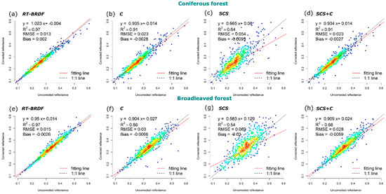
Figure 9.
Density scatterplots of the relationship between corrected and uncorrected BOA apparent reflectance at 837.19 nm for aspect perpendicular to the solar direction for coniferous (a–d) and broadleaved (e–h) forest. The best linear fit is in solid red, and the 1:1 line is in dashed blue.
4.4. BRDF Correction Assessment for Multiple-Flights
Although the C and SCS+C BRDF correction methods demonstrated to be able to effectively remove the topographic effects (Figure 9), RT-BRDF achieves a better correction of the BRDF effects between multiple flight-lines. For example, Figure 10a,b shows the difference between RT-BRDF corrected and C corrected reflectance at 837.19 nm for the third and second flight-line (06 April 2014), respectively. The RT-BRDF correction significantly reduced the back-scattering effects (i.e., west of the flight-line), whereas forward-scattering (i.e., east of the flight-line) reflectance is increased or maintained. In addition, differences in reflectance values are noticeable in the mosaicked difference image (Figure 10c) for regions overlapping adjacent flight-lines. Figure 10 provides an example of false color composite close ups of the results obtained with the different correction methods. Although SCS shows a tendency to overcorrect (i.e., bright pixels), all other correction methods are capable of removing the terrain-induced canopy BRDF distortions with varying degrees of success. However, the edge of a hyperspectral image is clearly noticeable in the uncorrected, C and SCS+C corrected mosaics, indicating a less than optimal compensation for the BRDF effects in overlapping regions. In contrast, the RT-BRDF corrected mosaic image shows a higher spectral homogeneity.
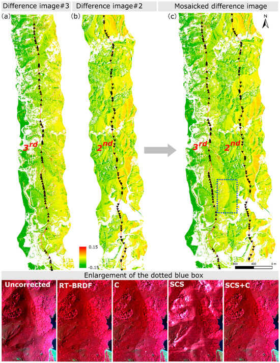
Figure 10.
Reflectance difference between RT-BRDF and C correction methods at 837.19 nm for (a) the third and (b) the second flight-lines (red line, with black arrows showing flight direction); (c) difference of mosaicked second and third flight-line and example close up (dotted blue box). Non-forested areas are in white. At the bottom, false-color composite close ups of the region delineated by the dotted blue box are shown.
This mitigation effect is further confirmed by the analysis of the RMSE of the variation in reflectance in the forested pixels (i.e., coniferous and broadleaved forest) from the overlap of two adjacent hyperspectral images. It clearly appears that the RMSE decreased post-RT-BRDF (Figure 11a,b), especially in the NIR region (i.e., >750 nm), implying that the selected forested areas shows more similar spectral values in the overlapped area of two images, and therefore an improvement in spectral homogeneity. The average decrease in RMSE of the spectra is 0.004 and 0.016 for coniferous forest and broadleaved forest, respectively.
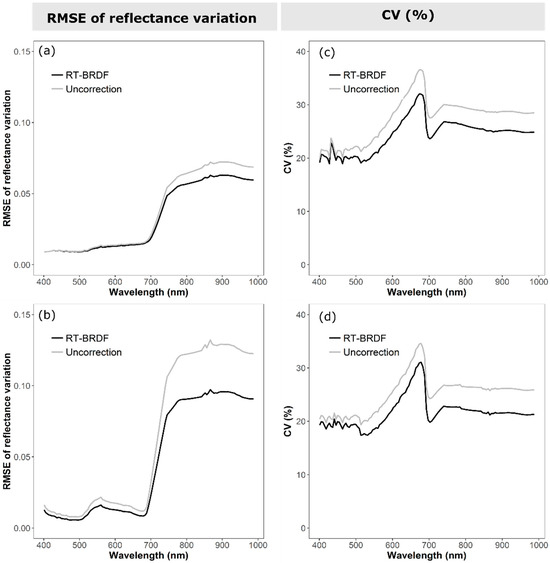
Figure 11.
Pre- and post-RT-BRDF RMSE of the reflectance values variability for (a) coniferous and (b) broadleaved forest pixels from adjacent and overlapping hyperspectral images. The coefficient of variation (CV) (%) of (c) coniferous and (d) broadleaved forest pre- and post-RT-BRDF.
A post-RT-BRDF reduction of the CV can also be observed for both coniferous (Figure 11c) and broadleaved forest (Figure 11d) at every wavelength. Specifically, the average decrease in CV is 3% and 3.5% for coniferous forest and broadleaved forest, respectively. In addition, it can be noticed that this reduction is more marked at longer wavelengths (i.e., NIR), and in particular in correspondence and after the characteristic green reflectance peak of vegetation (i.e., from ≈490 nm), with the exception of the maximum chlorophyll absorption wavelength (i.e., ≈680 nm; [7]).
4.5. MODIS BRDF Product Comparison
Figure 12a,b show the different sampling strategies of a multi-angle dataset for retrieving the kernel-based weighting parameters of AISA Eagle II and MODIS data, respectively. Then Figure 12c–e shows the comparison of the VHR pixel-based three BRDF model weighting parameters (, and ) of AISA Eagle II bands (400–990 nm) with the coarse scale (500 m) weighting parameters of MODIS bands 1–4, respectively. According to the strategies described in Section 3, the BRDF model weighting parameters of AISA Eagle II data are plotted for broadleaved forest and coniferous, respectively. Notably, all the BRDF model weighting parameters of broadleaved are slightly higher than those of coniferous in the visible (VIS) region but show much difference in the NIR region. The numerical ordering of the three weighting parameters is > > in each AISA Eagle II band for broadleaved forest and coniferous, respectively. A set of BRDF model weighting parameters for the corresponding MODIS bands 1–4 are generated, respectively, based on the relatively pure pixels with forest in the study area. The numerical ordering of the three weighting parameters is > > in each MODIS band. Generally, the of AISA Eagle II band is higher than the of MODIS band. Compared with the of AISA Eagle II band, the corresponding of MODIS band is slightly lower in the VIS region and significantly drops in the NIR region to be close to zero. Meanwhile, of AISA Eagle II band is nearly close to zero and much lower than the corresponding of MODIS band. The three weighting parameters present significant bias between AISA Eagle II and MODIS data in the NIR region but these are interestingly corrected.
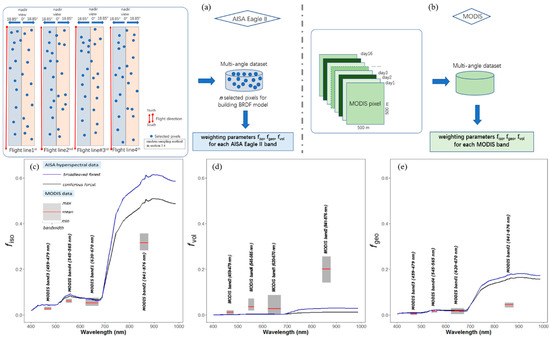
Figure 12.
Different sampling strategies of a multi-angle dataset for retrieval the kernel-based weighting parameters of Airborne Imaging Spectrometer for Applications (AISA) Eagle II (a) and Moderate Resolution Imaging Spectroradiometer (MODIS) (b) data. The comparison of the three BRDF model weighting parameters (c), (d), and (e) between AISA Eagle II and MODIS, respectively.
As illustrated in Figure 13a,c,d, both uncorrected and RT-BRDF corrected AISA Eagle II aggregated reflectance show similar correlations with the MODIS nadir BRDF-adjusted reflectance. In addition, these figures show both the uncorrected and RT-BRDF corrected AISA Eagle II aggregated reflectance are generally higher or lower than the MODIS reflectance. This may be caused by the lower signal-to-noise ratio of airborne hyperspectral images in the blue band or other upscaling issues which make reconstructing the BRDF accurately more challenging. Notably, the AISA Eagle II RT-BRDF corrected aggregated reflectance (Figure 13b) are more consistent with the MODIS nadir BRDF-adjusted reflectance in the NIR (MODIS band2; R2 = 0.83, RMSE = 0.007) showing a slightly higher consistency than the uncorrected scenario (R2 = 0.69, RMSE = 0.007).
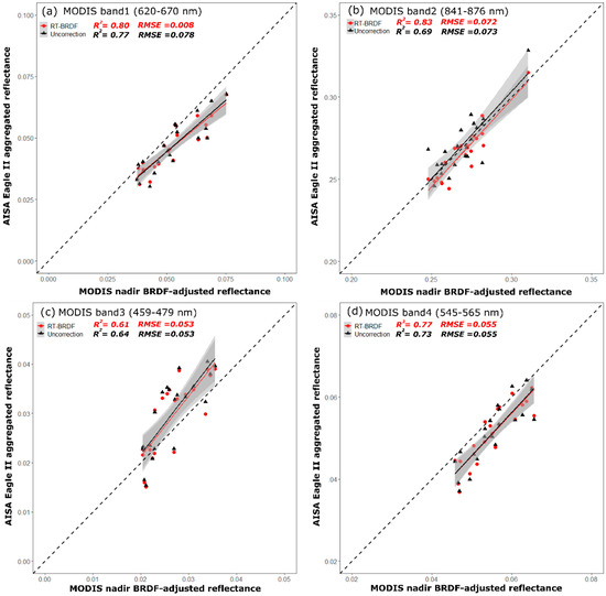
Figure 13.
Comparison between AISA Eagle II aggregated reflectance and MODIS nadir BRDF-adjusted reflectance corresponding band1-4 (a–d), respectively. The best linear fit is in solid red/black, and the 1:1 line is in dashed black.
4.6. Repeatability of the RT-BRDF Approach
Figure 14 shows the comparison of uncorrected and RT-BRDF corrected hyperspectral images of the 06 April 2014 flight campaign. Based on the full-sized observation of the image and the magnification of the selected areas, the RT-BRDF approach has the capability to reduce the BRDF effects caused by the combination of wide FOV airborne scanner and rugged topography in most forest covered areas. In addition, the RT-BRDF approach was utilized in another larger area hyperspectral images of the 04 April 2014 flight to verify the repeatability of the method. A cross-track brightness gradient is clearly discernible in the uncorrected data (Figure 15a) but it is almost entirely absent in the RT-BRDF corrected data (Figure 15b). The close-up areas (site A, B, and C) in Figure 15 show the goodness of the correction in greater detail.
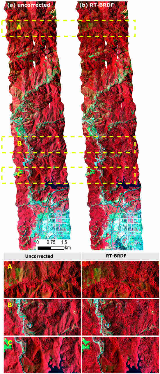
Figure 14.
The comparison of uncorrected and RT-BRDF corrected hyperspectral images of the 06/04/2014 flight mission displayed as false-color composites (i.e., 837.19, 694.91, 543.72 nm bands for the R, G, and B channels, respectively). (a) Uncorrected hyperspectral image; (b) post-RT-BRDF corrected hyperspectral image. The uncorrected and post-RT-BRDF corrected close-in images are shown for three selected sites (sites A, B, and C).
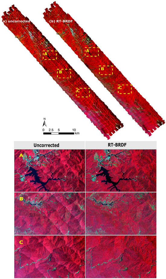
Figure 15.
The comparison of uncorrected and RT-BRDF corrected hyperspectral images of the 04/04/2014 flight mission displayed as false-color composites. (a) Uncorrected hyperspectral image; (b) post-RT-BRDF corrected hyperspectral image. The uncorrected and post-RT-BRDF corrected close-in images are shown for three selected sites (sites A, B, and C).
5. Discussion
The past two decades have seen significant advances in the use of airborne remote sensing data in the field of Earth system science and for ecosystem process modeling, from the canopy/stand level to more recently larger regions, increasing the demand for hyperspectral and LiDAR measurements. However, only few studies explored the applicability of BRDF correction methods to airborne hyperspectral imagery [6,7,92,93,94], especially for the forested areas with rugged topography. A better understanding of the BRDF effects on airborne hyperspectral imagery will provide clearer insights into their influence on remote sensing-based quantitative inversion products (e.g., LAI, PRI, canopy biochemistry parameters). In this study, we proposed an improved correction method for airborne hyperspectral imagery over rugged terrain with forest.
5.1. Inter-Comparison of BRDF Correction Methods
Several studies demonstrated how airborne imagery with high spatial resolution (i.e., 0.6–4.5 m) are significantly affected by BRDF effects and can only partly follow the standardized BRDF processing methods of satellite images (e.g., [7,15,42,95]). The results of our study further confirmed that slope-based volumetric and geometric kernels, which correct for both incident-angle-dependent and observation-angle-dependent BRDF effects, can be suitable for BRDF correction [47,48,76,77,96]. Especially, the improved RTM kernels (see Equation (11)) and LTR (see Equation (13)) demonstrated to be successful in BRDF correction for high resolution airborne imagery of forested areas with both flat [7] and rugged topography. With the exception of SCS, the topographic effects are effectively removed by RT-BRDF, C, and SCS+C (see Figure 6, Figure 7 and Figure 8). In fact, the SCS, which is a semi-physical method, failed in topographic correction under diffuse light conditions with an overcorrection of the reflectance [48,87,97]. Although the empirical, parameter-based C and SCS+C methods proved their effectiveness for topographic correction of satellite image, it remains challenging to utilize a universal empirical parameter C to correct images with varying topography and viewing-illumination geometries [48,87,98,99,100]. Both a visual inspection (Figure 6) and quantitative analysis (Figure 10) confirm that the empirical parameter-based methods are less than optimal for the BRDF correction of airborne images, especially for multiple flight-lines. In contrast, our results show that the physics-based RT-BRDF correction method can not only consistently compensate for terrain-induced but also for the viewing-illumination induced BRDF effects (Figure 11), which is supported by physical explanations (Figure 7 and Figure 9). Moreover, despite previous research based on the flat terrain hypothesis (e.g., [20,101,102]), it is demonstrated here the potential to correct the BRDF effects between multiple flight-lines images. The RT-BRDF approach opens the possibility of failures due to insufficient observations and/or poor angular sampling capability (e.g., [95]). Accounting for topography in the BRDF correction method still remains a largely unexplored task [7,19,42], but by design the limitations above do not affect the RT-BRDF method (Figure 4 and Figure 5).
5.2. Kernel-Driven BRDF Model Applied in Different Spatial Scales
Despite the spatial scaling assumptions underlying the semi-empirical kernel-driven BRDF approach for low spatial resolution [103], many studies demonstrated that it can be successful for reducing the BRDF effects of VHR airborne imagery [7,15,22,31,42]. However, only a few of these studies (i.e., [15]) give reasonable physical explanations for the applicability of the kernel-driven BRDF model with high spatial resolution imagery, which still needs further exploration. Results of Figure 12 show that for a coarse spatial resolution pixel such as 500 m of MODIS is dominated by the isotropic and volumetric scattering components. Likely, the geometric scattering component is inappropriate for the relief with a misrepresentation of shadowing effects in the observed scenes. It is reasonable that a MODIS pixel at this coarse-scale might contain many dense and continuous canopies in this study. Furthermore, a MODIS pixel contains both terrain-induced sunlit and shaded slope effects affecting the geometrical optics kernel in the kernel-driven BRDF modeling process (Figure 12b). Meanwhile, Figure 12 also reveals that a high spatial resolution pixel, such as for the VHR airborne imagery in this study (spatial resolution of 1 m), is more impacted by the isotropic and geometric components and less by the volumetric scattering component. A pixel of airborne image with ≈1 m resolution likely contains individual leaves and branches, and these physical attributes within the VHR pixels will lead to structure-induced mutual shadows within the canopy [15]. Moreover, topographic information, that differs from MODIS, was added to our RT-BRDF model which contributes to more geometric scattering effects of airborne imagery. It should be noticed that the cast-shaded pixels (deep gullies and canopy gaps) were ignored for the BRDF model reconstruction of airborne imagery in this study which could be the reason why of AISA Eagle II band has a higher value than of MODIS band. Ultimately, our results are consistent with other studies [43,104,105] suggesting that different scales can lead to different spatial and structural patterns containing different shadowing and clumping effects affecting the corresponding scattering component in the kernel-driven BRDF model.
Airborne hyperspectral images after RT-BRDF correction can reduce the reflectance in the back-scattering regions (or sunlit slope, if there is a mountain) and raise the reflectance in the forward-scattering regions (or shaded slope, if there is a mountain). While the RT-BRDF corrected airborne imagery performs better than the uncorrected images, there is no clear difference in Figure 13a,b. These results may be caused by the pixel aggregation process (500 m × 500 m) which averages the sunlit and shaded slope effects (swath width with ≈1000 m for one AISA Eagle II flight-line in this study). We therefore indicate that the airborne hyperspectral images under the acquisition conditions of this study have limited BRDF effects at course spatial resolutions (e.g., 500 m).
5.3. The Role of a Priori Knowledge on the BRDF Correction
Previous studies demonstrated that different land-cover types have different anisotropic properties and therefore different intrinsic BRDF characteristics [22,31,38,43]. Furthermore, the BRDF effects can vary with tree structure even within the same forest type [31,91]. While numerous studies use classification maps as a priori knowledge in the BRDF correction, this is by no means the only possible input [6,7,22]. A broader definition of a priori knowledge should contain external ancillary resources, such as field data, classification map, structure information, BRDF shapes from other products, topographic information, and ecological phenological season [38,86,106,107]. For example, for VHR airborne images, the structural information can be represented as texture based in algorithms such as GLCM, Sum Difference Histogram (SADH), and FOurier-based Textural Ordination (FOTO) [108,109]. Furthermore, the forest vertical and spatial structure can be derived from LiDAR data, such as canopy height, crown shape, as well as point cloud distribution of individual trees [110]. In this work, the general structure of the forest stand was investigated in the field, the classification map was produced using the SVM classification algorithm, and the high resolution DEM was derived directly from airborne LiDAR. Our results show that forest-type based reflectance is significantly different even for similar topographic conditions (Figure 8a,f), and as a consequence the BRDF models must be built separately. Due to the different structure of the coniferous and broadleaved forests in this study, it is possible to build accurate forest type-based BRDF models (Figure 5), leading to improved forest type-based correction results (Figure 7 and Figure 9). This further reinforces the fundamental role of a priori knowledge to describe the surface anisotropy based on multidimensional and temporal information in the BRDF correction.
5.4. Future Developments
Despite the RT-BRDF correction method for airborne hyperspectral imagery of forested areas with rugged topography was demonstrated to be successful across two study areas (Figure 14 and Figure 15), more investigations are needed to analyze how each factor affects the performance. Furthermore, additional research is needed to evaluate for sparse canopies and other land-cover types for different ecosystems. Although a combination of the RTM and LTR fixed kernels was chosen in our study, recent studies demonstrate that an adaptive kernels selection approach can improve the accuracy of BRDF models for different land-cover/structural types compared to fixed kernels [23,31]. In addition, the fitting method for BRDF modeling might also affect the correction result as mentioned in [22], especially for non-forest cover types such as wetlands and snow covered surfaces.
A typical hyperspectral flight has duration of 4-5 h and is influenced by varying sky conditions (i.e., the ratio of direct and diffuse radiation). However, because of the challenge to accurately describe the contribution of direct and diffuse irradiance to total irradiance in the actual operating process [32,33], in the RT-BRDF model we simplified this contribution by neglecting the influence of diffuse and adjacent surrounding radiance in the correction process. Another critical aspect of our study is that the CAF-LiCHy system was simultaneously acquired for both the airborne hyperspectral imagery and the LiDAR data, enabling the creation of an accurate high resolution LiDAR-derived DEM to describe the canopy and the underlying topography. In addition, the sensitivity analysis of the topographic correction with the DEM at different spatial scales highlighted the need for highly detailed DEMs to describe the physically based BRDF mechanism over rugged terrain [49,54]. This can be achieved using airborne systems integrating hyperspectral and LiDAR sensors. However, although the extremely high detail level of the DEM can trigger the characterization of fine scale topographic elements such as deep gullies and crags, it remains challenging to physically remove the shadow/cast-shadow effects due to varying irradiance.
Quantitative research on the correction of remotely sensed reflectance over rugged terrain has recently gained increasing attention, with the creation of new models such as the Kernel-Driven reflectance model for Sloping Terrain (KDST; [47]) and the Geometric-Optical model for Sloping Terrains (GOST; [111,112,113]). In addition, recent studies have worked towards a more accurate description of direct and diffuse irradiance components at the pixel level by considering a physically based approach with the combination of fine resolution DEM/DSM and the Discrete Anisotropic Radiative Transfer (DART) model [33,114].
6. Conclusions
In this study, we presented an improved kernel based BRDF correction operational framework for airborne hyperspectral images of forested areas with rugged topography (RT-BRDF). The RT-BRDF method is based on the multi-angular nature of aerial hyperspectral observations, caused by the combination of sensor scanning angles and topographic effects. In particular, the RT-BRDF method takes into account both the BRDF effects derived from topographic conditions and observation/solar incident angles, with the advantage of providing a physical meaning for the observed BRDF effects, differently from empirical and semi-physical topographic correction models. Additionally, a stratified random sampling method for the VHR airborne image with a large number of pixels can be an efficient way to ensure good representative of viewing and illumination angles through the minimum fitting error of the BRDF model for all bands (35,000 in this study). We demonstrated that, compared to other correction methods, RT-BRDF reduced the BRDF effects from multi-line aerial hyperspectral images of forested areas with rugged topography, and we believe that land-cover based models obtained using RT-BRDF have the potential to be applicable to large areas comprising numerous flight-lines. Results of this study can be used for reference in follow-up research and would contribute to reduce the limitation of large-scale applications of airborne hyperspectral data.
Author Contributions
Conceptualization, W.J. and Y.P.; Validation, W.J. and Y.P.; Investigation, W.J. and Y.P.; Writing—original draft preparation, W.J.; Writing—review and editing, W.J., Y.P., R.T., D.S., Z.L., J.-L.R.; Supervision, Y.P. and Z.L.; Project administration, Y.P. and Z.L. All authors have read and agreed to the published version of the manuscript.
Funding
This work was funded by the National Natural Science Foundation of China (31570546), Central Public-interest Scientific Institution Basal Research Found (No. CAFYBB2016ZD004) and the National High Technology Research and Development Program of China (No. 2012AA12A306).
Acknowledgments
We are particularly grateful to Zhihui Wang from Yellow River Institute of Hydraulic Research, Yellow River Conservancy Commission for his helpful discussions during the data processing. Thanks to Liangyun Liu, Jianguang Wen and Yadong Dong from Institute of Remote Sensing and Digital Earth (RADI), Chinese Academy of Sciences (CAS) for the assistance with writing of this article. We are thankful to the anonymous reviewers for valuable comments and suggestions to improve the manuscript.
Conflicts of Interest
The authors declare no conflict of interest.
References
- Chan, J.C.-W.; Paelinckx, D. Evaluation of Random Forest and Adaboost tree-based ensemble classification and spectral band selection for ecotope mapping using airborne hyperspectral imagery. Remote Sens. Environ. 2008, 112, 2999–3011. [Google Scholar] [CrossRef]
- Zhang, Y.; Chen, J.M.; Miller, J.R.; Noland, T.L. Leaf chlorophyll content retrieval from airborne hyperspectral remote sensing imagery. Remote Sens. Environ. 2008, 112, 3234–3247. [Google Scholar] [CrossRef]
- Goetz, A.F. Three decades of hyperspectral remote sensing of the Earth: A personal view. Remote Sens. Environ. 2009, 113, S5–S16. [Google Scholar] [CrossRef]
- Gatebe, C.K.; King, M.D. Airborne spectral BRDF of various surface types (ocean, vegetation, snow, desert, wetlands, cloud decks, smoke layers) for remote sensing applications. Remote Sens. Environ. 2016, 179, 131–148. [Google Scholar] [CrossRef]
- Schneider, F.D.; Morsdorf, F.; Schmid, B.; Petchey, O.L.; Hueni, A.; Schimel, D.S.; Schaepman, M.E. Mapping functional diversity from remotely sensed morphological and physiological forest traits. Nat. Commun. 2017, 8, 1441. [Google Scholar] [CrossRef] [PubMed]
- Weyermann, J.; Damm, A.; Kneubühler, M.; Schaepman, M.E. Correction of reflectance anisotropy effects of vegetation on airborne spectroscopy data and derived products. IEEE Trans. Geosci. Remote Sens. 2013, 52, 616–627. [Google Scholar] [CrossRef]
- Schläpfer, D.; Richter, R.; Feingersh, T. Operational BRDF effects correction for wide-field-of-view optical scanners (BREFCOR). IEEE Trans. Geosci. Remote Sens. 2014, 53, 1855–1864. [Google Scholar] [CrossRef]
- Ross, J.K. The Radiation Regime and Architecture of Plant Stands; Dr. W. Junk Publishers: Boston, UK, 1981; p. 392. [Google Scholar]
- Strahler, A.H.; Jupp, D.L. Modeling bidirectional reflectance of forests and woodlands using Boolean models and geometric optics. Remote Sens. Environ. 1990, 34, 153–166. [Google Scholar] [CrossRef]
- Liang, S.; Strahler, A.H. Retrieval of surface BRDF from multiangle remotely sensed data. Remote Sens. Environ. 1994, 50, 18–30. [Google Scholar] [CrossRef]
- Deering, D.W.; Eck, T.F.; Grier, T. Shinnery oak bidirectional reflectance properties and canopy model inversion. IEEE Trans. Geosci. Remote Sens. 1992, 30, 339–348. [Google Scholar] [CrossRef]
- Schaepman-Strub, G.; Schaepman, M.E.; Painter, T.H.; Dangel, S.; Martonchik, J.V. Reflectance quantities in optical remote sensing—Definitions and case studies. Remote Sens. Environ. 2006, 103, 27–42. [Google Scholar] [CrossRef]
- Nicodemus, F.E.; Richmond, J.C.; Hsia, J.J.; Ginsberg, I.; Limperis, T. Geometrical considerations and nomenclature for reflectance. NBS Monogr. 1992, 160, 4. [Google Scholar]
- Wen, J.; Liu, Q.; Xiao, Q.; Liu, Q.; You, D.; Hao, D.; Wu, S.; Lin, X. Characterizing land surface anisotropic reflectance over rugged terrain: A review of concepts and recent developments. Remote Sens. 2018, 10, 370. [Google Scholar] [CrossRef]
- Colgan, M.; Baldeck, C.; Féret, J.-B.; Asner, G. Mapping savanna tree species at ecosystem scales using support vector machine classification and BRDF correction on airborne hyperspectral and LiDAR data. Remote Sens. 2012, 4, 3462–3480. [Google Scholar] [CrossRef]
- Asner, G.P.; Wessman, C.A.; Privette, J.L. Unmixing the directional reflectances of AVHRR sub-pixel landcovers. IEEE Trans. Geosci. Remote Sens. 1997, 35, 868–878. [Google Scholar] [CrossRef]
- Asner, G.P.; Braswell, B.; Schimel, D.S.; Wessman, C.A. Ecological research needs from multiangle remote sensing data. Remote Sens. Environ. 1998, 63, 155–165. [Google Scholar] [CrossRef]
- Asner, G.P. Contributions of multi-view angle remote sensing to land-surface and biogeochemical research. Remote Sens. Rev. 2000, 18, 137–162. [Google Scholar] [CrossRef]
- Collings, S.; Caccetta, P.; Campbell, N.; Wu, X. Techniques for BRDF correction of hyperspectral mosaics. IEEE Trans. Geosci. Remote Sens. 2010, 48, 3733–3746. [Google Scholar] [CrossRef]
- Kennedy, R.E.; Cohen, W.B.; Takao, G. Empirical methods to compensate for a view-angle-dependent brightness gradient in AVIRIS imagery. Remote Sens. Environ. 1997, 62, 277–291. [Google Scholar] [CrossRef]
- Petri, C.A.; Galvão, L.S.; Lyapustin, A.I. MODIS BRDF effects over Brazilian tropical forests and savannahs: A comparative analysis. Remote Sens. Lett. 2019, 10, 95–102. [Google Scholar] [CrossRef]
- Jensen, D.J.; Simard, M.; Cavanaugh, K.C.; Thompson, D.R. Imaging spectroscopy BRDF correction for mapping Louisiana’s coastal ecosystems. IEEE Trans. Geosci. Remote Sens. 2017, 56, 1739–1748. [Google Scholar] [CrossRef]
- Guo, Y.; Jia, X.; Paull, D. Superpixel-based adaptive kernel selection for angular effect normalization of remote sensing images with kernel learning. IEEE Trans. Geosci. Remote Sens. 2017, 55, 4262–4271. [Google Scholar] [CrossRef]
- Koukal, T.; Atzberger, C.; Schneider, W. Evaluation of semi-empirical BRDF models inverted against multi-angle data from a digital airborne frame camera for enhancing forest type classification. Remote Sens. Environ. 2014, 151, 27–43. [Google Scholar] [CrossRef]
- Jiao, Z.; Dong, Y.; Schaaf, C.B.; Chen, J.M.; Román, M.; Wang, Z.; Zhang, H.; Ding, A.; Erb, A.; Hill, M.J. An algorithm for the retrieval of the clumping index (CI) from the MODIS BRDF product using an adjusted version of the kernel-driven BRDF model. Remote Sens. Environ. 2018, 209, 594–611. [Google Scholar] [CrossRef]
- Leckie, D.; Beaubien, J.; Gibson, J.; O’Neill, N.; Piekutowski, T.; Joyce, S. Data processing and analysis for MIFUCAM: A trial of MEIS imagery for forest inventory mapping. Can. J. Remote Sens. 1995, 21, 337–356. [Google Scholar] [CrossRef]
- Walthall, C.L. A study of reflectance anisotropy and canopy structure using a simple empirical model. Remote Sens. Environ. 1997, 61, 118–128. [Google Scholar] [CrossRef]
- Schiefer, S.; Hostert, P.; Damm, A. Correcting brightness gradients in hyperspectral data from urban areas. Remote Sens. Environ. 2006, 101, 25–37. [Google Scholar] [CrossRef]
- Rogge, D.; Bachmann, M.; Rivard, B.; Feng, J. Hyperspectral flight-line leveling and scattering correction for image mosaics. In Proceedings of the 2012 IEEE International Geoscience and Remote Sensing Symposium, Munich, Germany, 22–27 July 2012; pp. 4094–4097. [Google Scholar]
- Gastellu-Etchegorry, J.; Martin, E.; Gascon, F. DART: A 3D model for simulating satellite images and studying surface radiation budget. Int. J. Remote Sens. 2004, 25, 73–96. [Google Scholar] [CrossRef]
- Weyermann, J.; Kneubühler, M.; Schläpfer, D.; Schaepman, M.E. Minimizing Reflectance Anisotropy Effects in Airborne Spectroscopy Data Using Ross–Li Model Inversion with Continuous Field Land Cover Stratification. IEEE Trans. Geosci. Remote Sens. 2015, 53, 5814–5823. [Google Scholar] [CrossRef]
- Damm, A.; Guanter, L.; Paul-Limoges, E.; Van der Tol, C.; Hueni, A.; Buchmann, N.; Eugster, W.; Ammann, C.; Schaepman, M.E. Far-red sun-induced chlorophyll fluorescence shows ecosystem-specific relationships to gross primary production: An assessment based on observational and modeling approaches. Remote Sens. Environ. 2015, 166, 91–105. [Google Scholar] [CrossRef]
- Fawcett, D.; Verhoef, W.; Schläpfer, D.; Schneider, F.D.; Schaepman, M.E.; Damm, A. Advancing retrievals of surface reflectance and vegetation indices over forest ecosystems by combining imaging spectroscopy, digital object models, and 3D canopy modelling. Remote Sens. Environ. 2018, 204, 583–595. [Google Scholar] [CrossRef]
- Roujean, J.L.; Leroy, M.; Deschamps, P.Y. A bidirectional reflectance model of the Earth’s surface for the correction of remote sensing data. J. Geophys. Res. Atmos. 1992, 97, 20455–20468. [Google Scholar] [CrossRef]
- Wanner, W.; Strahler, A.; Hu, B.; Lewis, P.; Muller, J.P.; Li, X.; Schaaf, C.B.; Barnsley, M. Global retrieval of bidirectional reflectance and albedo over land from EOS MODIS and MISR data: Theory and algorithm. J. Geophys. Res. Atmos. 1997, 102, 17143–17161. [Google Scholar] [CrossRef]
- Schaaf, C.B.; Gao, F.; Strahler, A.H.; Lucht, W.; Li, X.; Tsang, T.; Strugnell, N.C.; Zhang, X.; Jin, Y.; Muller, J.-P. First operational BRDF, albedo nadir reflectance products from MODIS. Remote Sens. Environ. 2002, 83, 135–148. [Google Scholar] [CrossRef]
- Schaaf, C.; Liu, J.; Gao, F.; Strahler, A.H. MODIS albedo and reflectance anisotropy products from Aqua and Terra. Land Remote Sens. Glob. Environ. Chang. NASA’s Earth Obs. Syst. Sci. ASTER MODIS 2011, 11, 549–561. [Google Scholar]
- Roy, D.P.; Zhang, H.; Ju, J.; Gomez-Dans, J.L.; Lewis, P.E.; Schaaf, C.; Sun, Q.; Li, J.; Huang, H.; Kovalskyy, V. A general method to normalize Landsat reflectance data to nadir BRDF adjusted reflectance. Remote Sens. Environ. 2016, 176, 255–271. [Google Scholar] [CrossRef]
- Gemmell, F.; McDonald, A.J. View zenith angle effects on the forest information content of three spectral indices. Remote Sens. Environ. 2000, 72, 139–158. [Google Scholar] [CrossRef]
- Friedl, M.A.; Sulla-Menashe, D.; Tan, B.; Schneider, A.; Ramankutty, N.; Sibley, A.; Huang, X. MODIS Collection 5 global land cover: Algorithm refinements and characterization of new datasets. Remote Sens. Environ. 2010, 114, 168–182. [Google Scholar] [CrossRef]
- Bréon, F.-M.; Vermote, E. Correction of MODIS surface reflectance time series for BRDF effects. Remote Sens. Environ. 2012, 125, 1–9. [Google Scholar] [CrossRef]
- Wang, Z.; Liu, L. Correcting Bidirectional Effect for Multiple-Flightline Aerial Images Using a Semiempirical Kernel-Based Model. IEEE J. Sel. Top. Appl. Earth Obs. Remote Sens. 2016, 9, 4450–4463. [Google Scholar] [CrossRef]
- Román, M.O.; Gatebe, C.K.; Schaaf, C.B.; Poudyal, R.; Wang, Z.; King, M.D. Variability in surface BRDF at different spatial scales (30 m–500 m) over a mixed agricultural landscape as retrieved from airborne and satellite spectral measurements. Remote Sens. Environ. 2011, 115, 2184–2203. [Google Scholar] [CrossRef]
- Kharbouche, S.; Muller, J.-P.; Gatebe, C.; Scanlon, T.; Banks, A. Assessment of Satellite-Derived Surface Reflectances by NASA’s CAR Airborne Radiometer over Railroad Valley Playa. Remote Sens. 2017, 9, 562. [Google Scholar] [CrossRef]
- Lévesque, J.; King, D.J. Spatial analysis of radiometric fractions from high-resolution multispectral imagery for modelling individual tree crown and forest canopy structure and health. Remote Sens. Environ. 2003, 84, 589–602. [Google Scholar] [CrossRef]
- Clark, M.L.; Kilham, N.E. Mapping of land cover in northern California with simulated hyperspectral satellite imagery. ISPRS J. Photogramm. Remote Sens. 2016, 119, 228–245. [Google Scholar] [CrossRef]
- Wu, S.; Wen, J.; Gastellu-Etchegorry, J.-P.; Liu, Q.; You, D.; Xiao, Q.; Hao, D.; Lin, X.; Yin, T. The definition of remotely sensed reflectance quantities suitable for rugged terrain. Remote Sens. Environ. 2019, 225, 403–415. [Google Scholar] [CrossRef]
- Li, F.; Jupp, D.L.; Thankappan, M.; Lymburner, L.; Mueller, N.; Lewis, A.; Held, A. A physics-based atmospheric and BRDF correction for Landsat data over mountainous terrain. Remote Sens. Environ. 2012, 124, 756–770. [Google Scholar] [CrossRef]
- Zhang, Y.; Li, X.; Wen, J.; Liu, Q.; Yan, G. Improved topographic normalization for Landsat TM images by introducing the MODIS surface BRDF. Remote Sens. 2015, 7, 6558–6575. [Google Scholar] [CrossRef]
- Teillet, P.; Guindon, B.; Goodenough, D. On the slope-aspect correction of multispectral scanner data. Can. J. Remote Sens. 1982, 8, 84–106. [Google Scholar] [CrossRef]
- Richter, R. Correction of satellite imagery over mountainous terrain. Appl. Opt. 1998, 37, 4004–4015. [Google Scholar] [CrossRef]
- Riaño, D.; Chuvieco, E.; Salas, J.; Aguado, I. Assessment of different topographic corrections in Landsat-TM data for mapping vegetation types (2003). IEEE Trans. Geosci. Remote Sens. 2003, 41, 1056–1061. [Google Scholar] [CrossRef]
- Richter, R.; Kellenberger, T.; Kaufmann, H. Comparison of topographic correction methods. Remote Sens. 2009, 1, 184–196. [Google Scholar] [CrossRef]
- Feingersh, T.; Ben-Dor, E.; Filin, S. Correction of reflectance anisotropy: A multi-sensor approach. Int. J. Remote Sens. 2010, 31, 49–74. [Google Scholar] [CrossRef]
- Brook, A.; Polinova, M.; Ben-Dor, E. Fine tuning of the SVC method for airborne hyperspectral sensors: The BRDF correction of the calibration nets targets. Remote Sens. Environ. 2018, 204, 861–871. [Google Scholar] [CrossRef]
- Asner, G.P.; Knapp, D.E.; Kennedy-Bowdoin, T.; Jones, M.O.; Martin, R.E.; Boardman, J.W.; Field, C.B. Carnegie airborne observatory: In-flight fusion of hyperspectral imaging and waveform light detection and ranging for three-dimensional studies of ecosystems. J. Appl. Remote Sens. 2007, 1, 013536. [Google Scholar] [CrossRef]
- Kampe, T.U.; Johnson, B.R.; Kuester, M.A.; Keller, M. NEON: The first continental-scale ecological observatory with airborne remote sensing of vegetation canopy biochemistry and structure. J. Appl. Remote Sens. 2010, 4, 043510. [Google Scholar] [CrossRef]
- Cook, B.; Nelson, R.; Middleton, E.; Morton, D.; McCorkel, J.; Masek, J.; Ranson, K.; Ly, V.; Montesano, P. NASA Goddard’s LiDAR, hyperspectral and thermal (G-LiHT) airborne imager. Remote Sens. 2013, 5, 4045–4066. [Google Scholar] [CrossRef]
- Pang, Y.; Li, Z.; Ju, H.; Lu, H.; Jia, W.; Si, L.; Guo, Y.; Liu, Q.; Li, S.; Liu, L. LiCHy: The CAF’s LiDAR, CCD and hyperspectral integrated airborne observation system. Remote Sens. 2016, 8, 398. [Google Scholar] [CrossRef]
- Koetz, B.; Sun, G.; Morsdorf, F.; Ranson, K.; Kneubühler, M.; Itten, K.; Allgöwer, B. Fusion of imaging spectrometer and LIDAR data over combined radiative transfer models for forest canopy characterization. Remote Sens. Environ. 2007, 106, 449–459. [Google Scholar] [CrossRef]
- Dalponte, M.; Bruzzone, L.; Gianelle, D. Fusion of hyperspectral and LIDAR remote sensing data for classification of complex forest areas. IEEE Trans. Geosci. Remote Sens. 2008, 46, 1416–1427. [Google Scholar] [CrossRef]
- Jones, T.G.; Coops, N.C.; Sharma, T. Assessing the utility of airborne hyperspectral and LiDAR data for species distribution mapping in the coastal Pacific Northwest, Canada. Remote Sens. Environ. 2010, 114, 2841–2852. [Google Scholar] [CrossRef]
- Clark, M.L.; Roberts, D.A.; Ewel, J.J.; Clark, D.B. Estimation of tropical rain forest aboveground biomass with small-footprint lidar and hyperspectral sensors. Remote Sens. Environ. 2011, 115, 2931–2942. [Google Scholar] [CrossRef]
- Liu, L.; Coops, N.C.; Aven, N.W.; Pang, Y. Mapping urban tree species using integrated airborne hyperspectral and LiDAR remote sensing data. Remote Sens. Environ. 2017, 200, 170–182. [Google Scholar] [CrossRef]
- Li, Q.; Chen, Y.; Wang, S.; Zheng, Y.; Zhu, Y.; Wang, S. Diversity of ants in subtropical evergreen broadleaved forest in Pu’er City, Yunnan. Biodivers. Sci. 2009, 17, 233–239. [Google Scholar]
- Richter, R.; Schläpfer, D. Geo-atmospheric processing of airborne imaging spectrometry data. Part 2: Atmospheric/topographic correction. Int. J. Remote Sens. 2002, 23, 2631–2649. [Google Scholar] [CrossRef]
- Berk, A.; Cooley, T.W.; Anderson, G.P.; Acharya, P.K.; Bernstein, L.S.; Muratov, L.; Lee, J.; Fox, M.J.; Adler-Golden, S.M.; Chetwynd, J.H. MODTRAN5: A reformulated atmospheric band model with auxiliary species and practical multiple scattering options. In Proceedings of the Remote Sensing of Clouds and the Atmosphere 2005, Bruges, Belgium, 19–22 September 2005; pp. 78–85. [Google Scholar]
- Kayitakire, F.; Hamel, C.; Defourny, P. Retrieving forest structure variables based on image texture analysis and IKONOS-2 imagery. Remote Sens. Environ. 2006, 102, 390–401. [Google Scholar] [CrossRef]
- Lamonaca, A.; Corona, P.; Barbati, A. Exploring forest structural complexity by multi-scale segmentation of VHR imagery. Remote Sens. Environ. 2008, 112, 2839–2849. [Google Scholar] [CrossRef]
- Ozdemir, I.; Karnieli, A. Predicting forest structural parameters using the image texture derived from WorldView-2 multispectral imagery in a dryland forest, Israel. Int. J. Appl. Earth Obs. Geoinf. 2011, 13, 701–710. [Google Scholar] [CrossRef]
- Kozoderov, V.V.; Dmitriev, E.V. Testing different classification methods in airborne hyperspectral imagery processing. Opt. Express 2016, 24, A956–A965. [Google Scholar] [CrossRef]
- Dronova, I.; Gong, P.; Wang, L.; Zhong, L. Mapping dynamic cover types in a large seasonally flooded wetland using extended principal component analysis and object-based classification. Remote Sens. Environ. 2015, 158, 193–206. [Google Scholar] [CrossRef]
- Haralick, R.M.; Shanmugam, K.; Dinstein, I.H. Textural features for image classification. IEEE Trans. Syst. Manand Cybern. 1973, 610–621. [Google Scholar] [CrossRef]
- Clausi, D.A. An analysis of co-occurrence texture statistics as a function of grey level quantization. Can. J. Remote Sens. 2002, 28, 45–62. [Google Scholar] [CrossRef]
- Gao, B.; Jia, L.; Menenti, M. An improved method for retrieving land surface albedo over rugged terrain. IEEE Geosci. Remote Sens. Lett. 2013, 11, 554–558. [Google Scholar] [CrossRef]
- Schaaf, C.B.; Li, X.; Strahler, A.H. Topographic effects on bidirectional and hemispherical reflectances calculated with a geometric-optical canopy model. IEEE Trans. Geosci. Remote Sens. 1994, 32, 1186–1193. [Google Scholar] [CrossRef]
- Zhong, B.; Zhang, Y.; Du, T.; Yang, A.; Lv, W.; Liu, Q. Cross-Calibration of HJ-1/CCD over a desert site using landsat ETM $+ $ imagery and ASTER GDEM product. IEEE Trans. Geosci. Remote Sens. 2014, 52, 7247–7263. [Google Scholar] [CrossRef]
- Hilker, T.; Lyapustin, A.; Hall, F.G.; Wang, Y.; Coops, N.C.; Drolet, G.; Black, T.A. An assessment of photosynthetic light use efficiency from space: Modeling the atmospheric and directional impacts on PRI reflectance. Remote Sens. Environ. 2009, 113, 2463–2475. [Google Scholar] [CrossRef]
- Tortini, R.; Coops, N.; Nesic, Z.; Christen, A.; Lee, S.; Hilker, T. Remote sensing of seasonal light use efficiency in temperate bog ecosystems. Sci. Rep. 2017, 7, 8563. [Google Scholar] [CrossRef]
- Gao, F.; Li, X.; Strahler, A.; Schaaf, C. Evaluation of the Li transit kernel for BRDF modeling. Remote Sens. Rev. 2000, 19, 205–224. [Google Scholar] [CrossRef]
- Li, X.; Gao, F.; Chen, L.; Strahler, A.H. Derivation and validation of a new kernel for kernel-driven BRDF models. Remote. Sens. Earth Sci., Ocean., Sea Ice Appl. 1999, 3868, 368–379. [Google Scholar]
- Zhang, X.; Jiao, Z.; Dong, Y.; Zhang, H.; Li, Y.; He, D.; Ding, A.; Yin, S.; Cui, L.; Chang, Y. Potential investigation of linking PROSAIL with the ross-li BRDF model for vegetation characterization. Remote Sens. 2018, 10, 437. [Google Scholar] [CrossRef]
- Maignan, F.; Bréon, F.-M.; Lacaze, R. Bidirectional reflectance of Earth targets: Evaluation of analytical models using a large set of spaceborne measurements with emphasis on the Hot Spot. Remote Sens. Environ. 2004, 90, 210–220. [Google Scholar] [CrossRef]
- Padilla, M.; Stehman, S.V.; Ramo, R.; Corti, D.; Hantson, S.; Oliva, P.; Alonso-Canas, I.; Bradley, A.V.; Tansey, K.; Mota, B. Comparing the accuracies of remote sensing global burned area products using stratified random sampling and estimation. Remote Sens. Environ. 2015, 160, 114–121. [Google Scholar] [CrossRef]
- Boschetti, L.; Stehman, S.V.; Roy, D.P. A stratified random sampling design in space and time for regional to global scale burned area product validation. Remote Sens. Environ. 2016, 186, 465–478. [Google Scholar] [CrossRef] [PubMed]
- Li, A.; Wang, Q.; Bian, J.; Lei, G. An improved physics-based model for topographic correction of Landsat TM images. Remote Sens. 2015, 7, 6296–6319. [Google Scholar] [CrossRef]
- Yin, G.; Li, A.; Wu, S.; Fan, W.; Zeng, Y.; Yan, K.; Xu, B.; Li, J.; Liu, Q. PLC: A simple and semi-physical topographic correction method for vegetation canopies based on path length correction. Remote Sens. Environ. 2018, 215, 184–198. [Google Scholar] [CrossRef]
- Wen, J.; Liu, Q.; Liu, Q.; Xiao, Q.; Li, X. Parametrized BRDF for atmospheric and topographic correction and albedo estimation in Jiangxi rugged terrain, China. Int. J. Remote Sens. 2009, 30, 2875–2896. [Google Scholar] [CrossRef]
- Gu, D.; Gillespie, A. Topographic normalization of Landsat TM images of forest based on subpixel sun–canopy–sensor geometry. Remote Sens. Environ. 1998, 64, 166–175. [Google Scholar] [CrossRef]
- Soenen, S.A.; Peddle, D.R.; Coburn, C.A. SCS+C: A modified sun-canopy-sensor topographic correction in forested terrain. IEEE Trans. Geosci. Remote Sens. 2005, 43, 2148–2159. [Google Scholar] [CrossRef]
- Jia, W.; Coops, N.C.; Tortini, R.; Pang, Y.; Black, T.A. Remote sensing of variation of light use efficiency in two age classes of Douglas-fir. Remote Sens. Environ. 2018, 219, 284–297. [Google Scholar] [CrossRef]
- Wetherley, E.B.; Roberts, D.A.; McFadden, J.P. Mapping spectrally similar urban materials at sub-pixel scales. Remote Sens. Environ. 2017, 195, 170–183. [Google Scholar] [CrossRef]
- Tane, Z.; Roberts, D.; Veraverbeke, S.; Casas, Á.; Ramirez, C.; Ustin, S. Evaluating endmember and band selection techniques for multiple endmember spectral mixture analysis using post-fire imaging spectroscopy. Remote Sens. 2018, 10, 389. [Google Scholar] [CrossRef]
- Meerdink, S.K.; Roberts, D.A.; Roth, K.L.; King, J.Y.; Gader, P.D.; Koltunov, A. Classifying California plant species temporally using airborne hyperspectral imagery. Remote Sens. Environ. 2019, 232, 111308. [Google Scholar] [CrossRef]
- Jiao, Z.; Zhang, H.; Dong, Y.; Liu, Q.; Xiao, Q.; Li, X. An algorithm for retrieval of surface albedo from small view-angle airborne observations through the use of BRDF archetypes as prior knowledge. IEEE J. Sel. Top. Appl. Earth Obs. Remote Sens. 2015, 8, 3279–3293. [Google Scholar] [CrossRef]
- Wen, J.; Liu, Q.; Tang, Y.; Dou, B.; You, D.; Xiao, Q.; Liu, Q.; Li, X. Modeling land surface reflectance coupled BRDF for HJ-1/CCD data of rugged terrain in Heihe river basin, China. IEEE J. Sel. Top. Appl. Earth Obs. Remote Sens. 2015, 8, 1506–1518. [Google Scholar] [CrossRef]
- Kane, V.R.; Gillespie, A.R.; McGaughey, R.; Lutz, J.A.; Ceder, K.; Franklin, J.F. Interpretation and topographic compensation of conifer canopy self-shadowing. Remote Sens. Environ. 2008, 112, 3820–3832. [Google Scholar] [CrossRef]
- Wu, J.; Bauer, M.E.; Wang, D.; Manson, S.M. A comparison of illumination geometry-based methods for topographic correction of QuickBird images of an undulant area. ISPRS J. Photogramm. Remote Sens. 2008, 63, 223–236. [Google Scholar] [CrossRef]
- Vanonckelen, S.; Lhermitte, S.; Van Rompaey, A. The effect of atmospheric and topographic correction methods on land cover classification accuracy. Int. J. Appl. Earth Obs. Geoinf. 2013, 24, 9–21. [Google Scholar] [CrossRef]
- Moreira, E.P.; Valeriano, M.M. Application and evaluation of topographic correction methods to improve land cover mapping using object-based classification. Int. J. Appl. Earth Obs. Geoinf. 2014, 32, 208–217. [Google Scholar] [CrossRef]
- Beisl, U. BRDF Correction in Hyperspectral Imagery. Digit. Airborne Spectrometer Exp. 2001, 499, 177. [Google Scholar]
- López, D.H.; García, B.F.; Piqueras, J.G.; Alcázar, G.V. An approach to the radiometric aerotriangulation of photogrammetric images. ISPRS J. Photogramm. Remote Sens. 2011, 66, 883–893. [Google Scholar] [CrossRef]
- Lucht, W.; Roujean, J.L. Considerations in the parametric modeling of BRDF and albedo from multiangular satellite sensor observations. Remote Sens. Rev. 2000, 18, 343–379. [Google Scholar] [CrossRef]
- d’Entremont, R.P.; Schaaf, C.B.; Lucht, W.; Strahler, A.H. Retrieval of red spectral albedo and bidirectional reflectance using AVHRR HRPT and GOES satellite observations of the New England region. J. Geophys. Res. Atmos. 1999, 104, 6229–6239. [Google Scholar] [CrossRef]
- Walthall, C.; Roujean, J.L.; Morisette, J. Field and landscape BRDF optical wavelength measurements: Experience, techniques and the future. Remote Sens. Rev. 2000, 18, 503–531. [Google Scholar] [CrossRef]
- Li, X.; Strahler, A. A knowledge-based inversion of physical BRDF model and three examples. In Proceedings of the IGARSS’96. 1996 International Geoscience and Remote Sensing Symposium, Lincoln, NE, USA, 31 May 1996; pp. 2173–2176. [Google Scholar]
- Li, X.; Gao, F.; Wang, J.; Strahler, A. A priori knowledge accumulation and its application to linear BRDF model inversion. J. Geophys. Res. Atmos. 2001, 106, 11925–11935. [Google Scholar] [CrossRef]
- Couteron, P.; Pelissier, R.; Nicolini, E.A.; Paget, D. Predicting tropical forest stand structure parameters from Fourier transform of very high-resolution remotely sensed canopy images. J. Appl. Ecol. 2005, 42, 1121–1128. [Google Scholar] [CrossRef]
- Meng, S.; Pang, Y.; Zhang, Z.; Jia, W.; Li, Z. Mapping aboveground biomass using texture indices from aerial photos in a temperate forest of Northeastern China. Remote Sens. 2016, 8, 230. [Google Scholar] [CrossRef]
- Lindberg, E.; Holmgren, J. Individual tree crown methods for 3D data from remote sensing. Curr. For. Rep. 2017, 3, 19–31. [Google Scholar] [CrossRef]
- Fan, W.; Chen, J.M.; Ju, W.; Zhu, G. GOST: A geometric-optical model for sloping terrains. IEEE Trans. Geosci. Remote Sens. 2013, 52, 5469–5482. [Google Scholar]
- Fan, W.; Li, J.; Liu, Q. GOST2: The improvement of the canopy reflectance model GOST in separating the sunlit and shaded leaves. IEEE J. Sel. Top. Appl. Earth Obs. Remote Sens. 2015, 8, 1423–1431. [Google Scholar] [CrossRef]
- Fan, W.; Li, J.; Liu, Q.; Zhang, Q.; Yin, G.; Li, A.; Zeng, Y.; Xu, B.; Xu, X.; Zhou, G. Topographic Correction of Forest Image Data Based on the Canopy Reflectance Model for Sloping Terrains in Multiple Forward Mode. Remote Sens. 2018, 10, 717. [Google Scholar] [CrossRef]
- Schläpfer, D.; Hueni, A.; Richter, R. Cast shadow detection to quantify the aerosol optical thickness for atmospheric correction of high spatial resolution optical imagery. Remote Sens. 2018, 10, 200. [Google Scholar] [CrossRef]
© 2020 by the authors. Licensee MDPI, Basel, Switzerland. This article is an open access article distributed under the terms and conditions of the Creative Commons Attribution (CC BY) license (http://creativecommons.org/licenses/by/4.0/).