Article

Temperature and Humidity Profiles Retrieval in a Plain Area from Fengyun-3D/HIRAS Sensor Using a 1D-VAR Assimilation Scheme

1
Collaborative Innovation Center on Forecast and Evaluation of Meteorological Disasters, CMA Key Laboratory for Aerosol-Cloud-Precipitation, Nanjing University of Information Science & Technology, Nanjing 210044, China
2
School of Atmospheric Physics, Nanjing University of Information Science & Technology, Nanjing 210044, China
3
School of Mineral Resources Engineering, Technical University of Crete, Kounoupidiana Campus, 73100 Crete, Greece
4
Department of Geography, Harokopio University of Athens, El. Venizelou 70, Kallithea, 17671 Athens, Greece
5
Key Laboratory of Radiometric Calibration and Validation for Environmental Satellites /National Satellite Meteorological Center, China Meteorological Administration, Beijing 100081, China
*
Author to whom correspondence should be addressed.
Remote Sens. 2020, 12(3), 435; https://doi.org/10.3390/rs12030435
Submission received: 22 November 2019 / Revised: 30 December 2019 / Accepted: 13 January 2020 / Published: 29 January 2020
(This article belongs to the Section Atmospheric Remote Sensing)

Abstract

:
In this study, a one-dimensional variational (1D-VAR) retrieval system is proposed to simultaneously retrieve temperature and humidity atmospheric profiles under clear-sky conditions. Our technique requires observations from the Fengyun-3D Hyperspectral Infrared Radiation Atmospheric Sounding (HIRAS) satellite combined with the Weather Research and Forecast (WRF) model. In the method, the radiative transfer for the TIROS Operational Vertical Sounder (TOVS (RTTOV) model is also used as a forward observation operator. The accuracy of our approach was evaluated using as a case study the region of Beijing in China. Predicted temperature and humidity profiles were compared against ERA-Interim data, which was used as reference. Mean bias (MB) of the temperature profiles varied between −0.8 K to 0.9 K, while the root-mean-square error (RMSE) ranged from 0.5 K to 2.6 K. In the boundary layer, the 1D-VAR algorithm performed better compared with the first guess. In the middle troposphere, the retrievals were more dependent on the first guess. With respect to relative humidity predictions, the accuracy of the evaluation of the whole troposphere was improved with the inclusion of the satellite observations, reporting an MB varying from −5.68% to 2.83%. Compared with Atmospheric Infrared Sounder’s (AIRS’) products, our predicted temperature profiles showed a very good consistency and the humidity predictions were also of an acceptable prediction accuracy. All in all, results clearly evidenced the promising potential of our proposed approach for retrieving temperature and humidity profiles under clear-sky conditions.

1. Introduction

Atmospheric temperature and humidity profiles are important parameters in the atmospheric system. Accurate information on those parameters is required for improving the accuracy of numerical weather predictions [1] and short-term weather warnings [2]. At present, atmospheric temperature and humidity profiles can be directly measured using radiosondes. Yet, due to the low spatial resolution, the uneven distribution of sounding stations around the world, and the lack of information at a higher level, it is difficult to meet the requirements of operational use on variable geographical scales. The recent emergence of infrared (IR) hyperspectral vertical detectors opens up a new era in the use of satellite data for this purpose. The information obtained using infrared hyperspectral vertical detectors is hundreds of times richer spectrally in comparison to ordinary meteorological satellites. It can also display a more detailed atmospheric structure, which provides important information toward improving the accuracy of the retrievals of atmospheric temperature and humidity profiles. Satellite IR remote sensing offers an indirect measurement of atmospheric temperature and moisture [3]. Combining the IR radiation transmission model with a retrieval algorithm, the temperature and humidity profiles can be obtained using the radiation received by IR sensors.
The main retrieval methods used for this purpose nowadays include eigenvector statistics, artificial neural networks, and the variational method. Not long ago, Smith and Woolf [4] proposed a new technique for retrieving atmospheric parameters from spectral radiance observations using eigenvector covariance matrices. Other scholars [5,6,7,8] have used eigenvector statistics in atmospheric temperature and humidity profile retrievals from the Atmospheric Infrared Sounder (AIRS). Results from those studies suggested that the inclusion of information from hyperspectral atmospheric vertical sounding instruments can offer important information that helps in improving the retrieval accuracy of information about the upper and middle troposphere. However, this method does not consider the physical nature of atmospheric radiation transmission, which affects the retrieval accuracy. Neural networks have also been used for this purpose [9,10,11]. For example, Singh [12] retrieved atmospheric temperature and humidity profiles by using neural networks based on a Advanced Microwave Sounding Unit (AMSU). In their study, the authors reported a close agreement of the predicted temperature and humidity profiles when compared against measurements from the Atmospheric Infrared Sounder (AIRS), with a bias under 850 hPa of 3 K and 4 g/kg, respectively. Nonetheless, their proposed method was dependent on a large training dataset, a condition that may not always be met in practical implementation scenarios [13]. The variational method takes the atmospheric radiation transmission into account and it does not depend on the training samples’ properties. It allows for the retrieval of the vertical distribution of atmospheric temperature and humidity by means of combining observation values, prior values, and error information together [14,15,16]. Li [17,18] used AIRS simulation data to obtain the analytical form of the atmospheric temperature and water vapor weight function under clear-sky conditions based on the 1D-VAR principle. He then obtained the linearized radiation transmission equation and assessed the atmospheric temperature and moisture profile through Newton non-linear iterations. Results of this study reported an accuracy of 1 K in temperature and 10% in water vapor retrieval when compared against AIRS simulated data. Since then, many scholars have used 1D-VAR to obtain atmospheric variables and developed assimilation systems for a variety of microwave sensors [19,20], IR hyperspectral vertical detectors [21], and ground-based microwave radiometer [22].
In purview of the above, this study aims at introducing a new temperature and humidity retrieval approach for use with the FY-3D/HIRAS, the Chinese next generation polar meteorological satellite. The system is based on a 1D-VAR assimilation method combined with the Weather Research and Forecast (WRF) model and Radiative Transfer for the TIROS Operational Vertical Sounder (TOVS) (RTTOV). A deep learning method has also been adopted to conduct cloud detection, which provides an important asset for our proposed method toward a potential operationalization of its implementation.

2. Datasets and Model

2.1. Fengyun-3D Hyperspectral Infrared Radiation Atmospheric Sounding (FY-3D/HIRAS) Data and Pre-Processing

Fengyun 3 series is the second generation of Chinese sun-synchronous meteorological satellites [23]. The fourth satellite, FY-3D, was launched on 15 November 2017, operating at an altitude of 830.5 km and at an orbital tilt angle of 98.6°. In contrast to the previous FY-3A/B/C satellites, FY-3D is able to provide more multi-spectral observations under all weather conditions. It has 10 sensors on board. It has two new IR high-spectral sensors with more than 2000 channels, where one is HIRAS and another is the Greenhouse Gases Absorption Spectrometer (GAS) [24]. Also, for the first time, FY-3D is carrying infrared Fourier detection instruments. HIRAS has a spectral range from 0.38 microns to 15.38 microns. The instrument’s observation spectrum is divided into three infrared spectrum bands: long wave (LW), medium wave 1 (MW1), and medium wave 2 (MW2); the spectral characteristics are summarized below (Table 1).
The HIRAS observation mode is shown in Figure 1. Each scanning line observes 33 FORs (fields of regard), including 4 probes arranged in a 2 × 2 array, and each probe is called a FOV (field of view). Due to the channel spectral response function caused by the interference instrument’s finite optical path difference, the channel spectral radiation has a side-lobe effect. In order to suppress it, multiple apodization methods are available. The three-point sliding average filtering, called the Hamming function, is one of them, with coefficients of 0.23, 0.54, and 0.23. Figure 2 shows the apodization effect on satellite radiation observation. In our study, the observation data used in the establishment of the 1D-VAR retrieval algorithm came from the HIRAS L1-level orbital data acquired over the Beijing region from July to December 2018.

2.2. WRF Model

The temperature and humidity profiles retrieval is an ill-posed problem because there are an infinite number of atmospheric states that can produce a given observation vector within its uncertainty [14]. This problem can be formalized from the viewpoint of the conditional, or Bayesian, probabilities. The aim is to find the most likely state of the atmosphere with the observation vectors known, which is described mathematically as follows:
max ( P ( x | Y ) )
P ( x | Y )   =   P ( Y | x ) P ( x ) P ( Y ) ,
where x presents the atmospheric state vector and Y is the observation vector. P(xǀY) is denoted as the probability that x occurs when Y occurs, and vice versa. In the analysis procedure, we know that a measurement has been made and we know its value Y, so P(Y) = 1 and we obtain:
P ( x | Y )   =   P ( Y | x ) P ( x ) ,
which means that the analysis probability density function (pdf) is equal to the background pdf times the observation pdf. The term P(x) in Equation (3) is the a priori pdf of the model state before the observations are considered (i.e., the background pdf). Based on the Bayes theorem, the WRF mesoscale numerical forecast model is used to provide background data for the retrieval of temperature and humidity profiles. The boundary and initial conditions are provided by the reanalysis data produced by the National Center for Environmental Prediction (NCEP) and National Center for Atmospheric Research (NCAR) at the time of 0:00 UTC each day, and the output of the model is a 6-hour simulation time step. The simulation results at 5:00 UTC are extracted, and the grid point data of the model are interpolated to the satellite observation positions. In the retrieval process, the number of the profile layers is set to 88 and the pressure distribution range is set between 1 and 1000 hPa. Therefore, it is necessary to interpolate the output atmospheric state vector to the uniform pressure layer.

2.3. RTTOV Model

A forward model is needed to transform the atmospheric state vector into the observation space. In our study, RTTOV was used. RTTOV is a development of the fast radiative transfer model for TOVS, originally developed at ECMWF (European Centre for Medium-Range Weather Forecasts) in the early 1990s [25] to simulate spectral radiance in infrared and microwave TOVS. On the basis of atmospheric transmittance, RTTOV can calculate the rapid radiation transmission in a clear sky [26]. Some actual profiles are needed to simulate the correct brightness temperature. In this algorithm, the output result of WRF can be used as an input for RTTOV. The number of simulation layers is also set to 88, which is consistent with the profile from the RTTOV model. The surface emissivity is also calculated by the model based on surface types from the WRF output (instead of provided directly by the user).

3. Development of a 1D-VAR Assimilation System

3.1. Retrieval Algorithm Mathematical Background

The one-dimension variation method employed herein is similar to the variational radiance data assimilation in the numerical weather prediction (NWP) model. It is performed by adjusting the atmospheric state vector x from the background state xb to minimize a cost function of the following form [27]:
J ( x )   =   1 2 [ ( x     x b ) T · B 1 · ( x     x b ) ]   +   1 2 [ ( Y     ( F ( x ) ) T · O 1 · ( Y     F ( x ) ) ] ,
where B and O represent the background error covariance matrix and observation error covariance matrix, respectively. F is the forward model operator (RTTOV in this study) and Y is the brightness temperature from HIRAS. The first term on the right represents the penalty for departing from the a priori information, while the second term represents the penalty for departing from the measurements. The cost function needs to be minimized for retrieving the temperature and humidity profiles. Common minimization algorithms include the gradient descent method, conjugate gradient method, Newton method, and quasi-Newton method, etc. Herein, the Newton method was adopted to seek the minimum value of objective function with the help of partial derivative information [28] as it has the second order convergence, on which the convergence speed is faster than other similar methods. Its iterative equation is expressed as follows:
x n + 1   =   x n     ( 2 J ( x n ) x n 2 ) 1 · J ( x n ) x n ,
where the first and second partial derivatives of the cost function are:
J ( x ) ( x )   =   B 1 · ( x     x b )     K T · O 1 · ( Y     F ( x ) ) ,
2 J ( x ) x 2   =   B 1   +   K T · O 1 · K     2 F ( x ) x 2 · O 1 · ( Y     F ( x ) ) ,
where K is the Jacobian. In view of the increasingly close Y and F(x) in the iterative process, in order to reduce the computational amount, the term with (Y – F(x)) in the second partial derivative is often ignored [17].
The final iteration equation is:
x n + 1   =   x n   +   ( B 1   +   K T · O 1 · K ) 1 · [ B 1 · ( x b     x n )   +   K T · O 1 · ( Y     F ( x n ) ) ] ,
where n is the iteration index. xn and xn+1 represent the profiles of the atmospheric temperature and humidity at steps n and n+1, respectively, in the iteration process. However, the initial value selection in the Newton method implementation is crucial. If the initial values are far away from the optimal solution, the algorithm will fail to converge. For this reason, the global Newton method, in which the Armijo rule is introduced in the process of the optimal solution search to ensure that each search step length is the most appropriate, is employed as follows:
x n + 1   =   x n   +   α · ( B 1   +   K T · O 1 · K ) 1 · [ B 1 · ( x b     x n ) + K T · O 1 · ( Y     F ( x n ) ) ] ,
where α represents the iteration step length. There are two core ideas in the Armijo rule. One is that the value of the coat function should decrease, and another is that α should not be too small. According to these, α should meet the following two equations:
f ( x n + 1 )     f ( x n )   +   α n ρ g n T d n ,
f ( x n + 1 )     f ( x n )   +   α n ( 1     ρ ) g n T d n ,
where f represents the cost function, αn is the step length at step n, gn is the first order of the cost function (Equation (6)) at step n, and the superscript T represents transpose. The value of ρ can be set between 0 and 0.5 to ensure the superlinear convergence of the algorithm. dn can be written as:
d n   =   ( B 1   +   K T · O 1 · K ) 1 · [ B 1 · ( x b     x n )   +   K T · O 1 · ( Y     F ( x n ) ) ] ,
Finally, the termination condition of the iteration (Equation (9)) is expressed as follows:
x n     x n + 1 2 <   0.05 ,

3.2. Cloud-Screening

Cloud cover has a strong effect on IR radiance measurements [29]. Therefore, cloud pixels need to be removed before using hyperspectral data for retrieval. In our study, a cloud detection model is developed using a classification algorithm based on the GBDT (gradient boosting decision tree). Gradient boosting machine learning belongs to a family of powerful machine learning techniques that have shown considerable success in a wide range of practical applications. They are highly customizable to the particular needs of the application, such as being learned with respect to different loss functions [30]. Multiple decision trees are involved in the decision making, and the residual error (i.e., the deviation between the conclusion and the true value) of all trees before each tree is learned is added up to give the final result. As the output sample value is not continuous, we cannot fit errors of the output category directly. To solve this, the logarithm likelihood loss function was employed. This means that a category prediction probability value and the difference in the real probability value for fitting the loss was used in our study. The input parameters for the model included the brightness temperature of each channel, the satellite observation angle, and the solar altitude angle information, while the output parameters were the cloud/cloudless discriminate markers.

3.3. Channel Selection

There are thousands of infrared hyperspectral channels and if all channels are used in the algorithm, this will limit the computational resources and computing time will be increased. Therefore, the optimal temperature and humidity retrieval channels need to be selected.
The method adopted for this in our approach is the weight function covering method. It calculates the Jacobian matrix of each channel, described as follows:
δ y   =   H ( x 0 ) δ x .
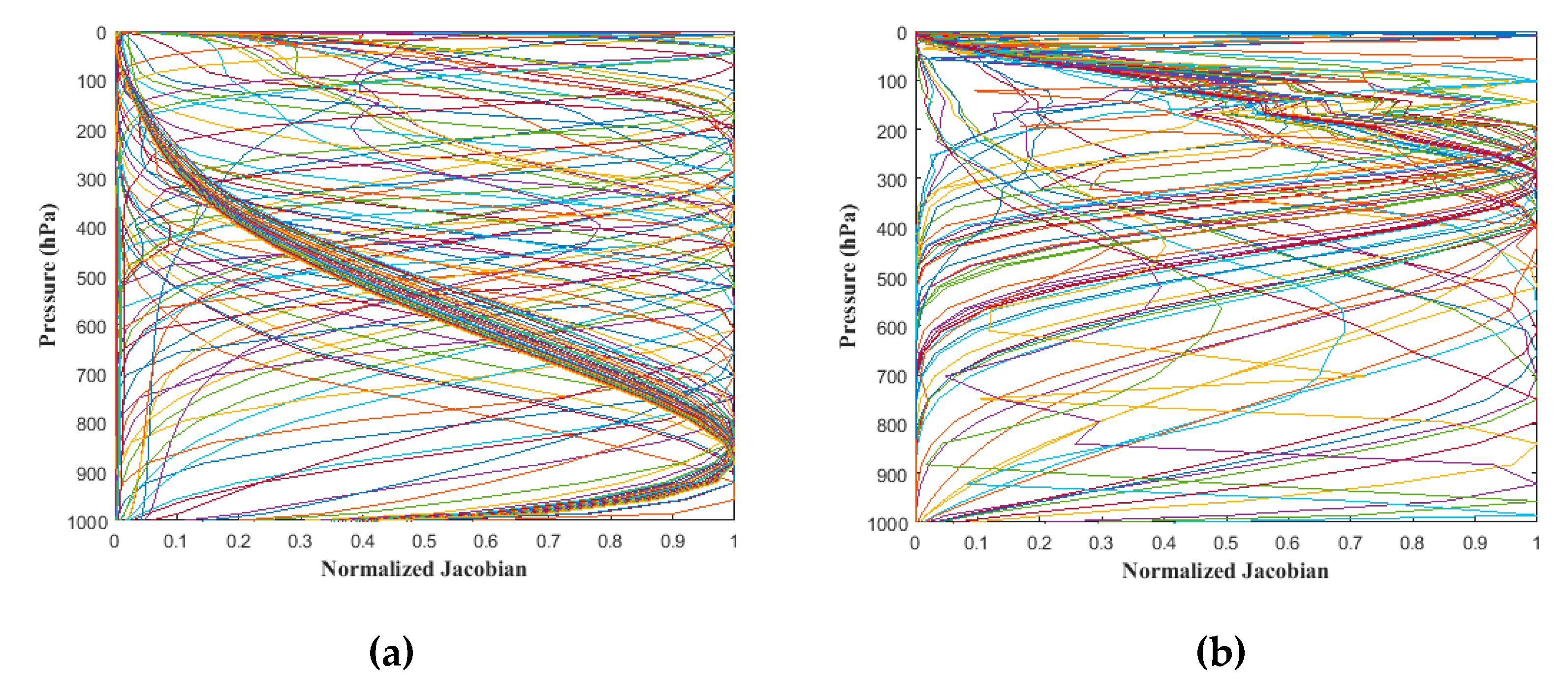
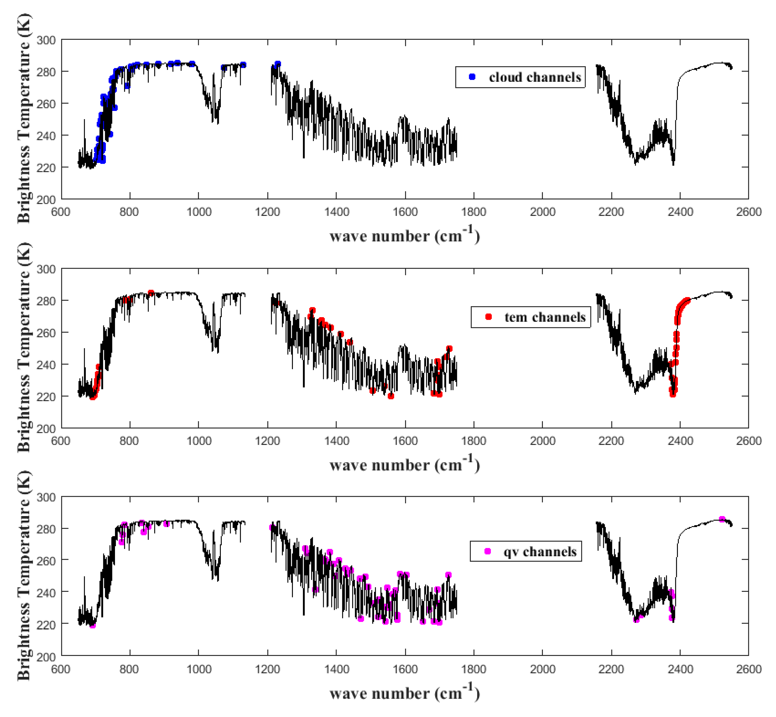
The H elements contain the partial derivatives ∂yi/∂xj where the subscript i refers to the channel number and j refers to the position in the state vector. The Jacobian gives the top-of-atmosphere radiance change for each channel given unit perturbations at each respective level of the profile vectors and in each of the surface/cloud parameters. It shows clearly for a given profile which layers in the atmosphere are most sensitive to changes in temperature and variable gas concentrations for each channel. Channel selection is based on the linear width, peak position, and peak size of the channel weight function [31]. The steeper the weight function, the higher the contribution of the radiation energy in the atmosphere to the satellite detection instrument from the pressure layer where the peak layer is located. Meanwhile, the higher the weight function peak value, the higher the contribution of radiation energy to the sensor from the pressure layer where the peak layer is located. When the channels’ peak layers are in the middle troposphere and above, the channel with the highest peak value will be selected if different channels have the same peak layer. As for channels with a peak value layer of the weight function in the lower troposphere, considering that the errors of the lower troposphere and near ground are large, two channels are selected: one focuses on the steep linear shape and the other focuses on the peak value. In our study, the atmospheric profile input to RTTOV for channel selection is a mean of the diverse profiles from the ERA-Interim data in the Beijing area on 29 September 2018, 4 October 2018, and 21 November 2018 under clear-sky cases. The final selected weight functions of the temperature and humidity channels are shown in Figure 3. It is worth noting that the abscissa is the normalized Jacobian. The cloud detection channels are set according to the AIRS channel settings. Finally, 51 cloud channels, 80 temperature channels, and 56 humidity channels were chosen. The channel selection is shown in Figure 4.

3.4. Background Error Covariance Matrix Localization

The background error covariance B describes the accepted variance at each level between the forecast and the true atmospheric state vector, as well as the correlations between them [14]. Background error covariance is one of the most important parts in one-dimensional variation, which determines the degree to which the observation is revised to the background [32]. If the background error covariance matrix B is overestimated, the role of the background term in the objective function will be reduced. Consequently, the results of the analysis field will be closer to the observation field information and better background information will be ignored. Conversely, if the effect of the observation term in the objective function is reduced, then the results of the analysis field will be closer to the background field and the information of the good observation field will be ignored, such that the purpose of assimilation fails to be achieved.
The two main methods to generate the background error covariance include the statistical [33] and National Meteorological Center (NMC) [34] methods. The first compares the simulated background field with the real value, which can be the radio sounding data. However, limitations of this method include the uneven distribution of sounding data and the lack of information at higher levels t; herein, the second method is used to produce the background error covariance matrix in this study. It is assumed that the statistical structure of the prediction error of the model changes very little within a fixed forecast time. In this way, the difference between forecast values of different forecast times at the same instance can be used as the background error. Its advantage is that it is not limited by the resolution of the observation network and the background error covariance features can be used for the global scale. Mathematically, it is expressed as follows:
B   =   ( x b     x t ) ( x b     x t ) T ¯     α ( x 24     x 12 ) ( x 24     x 12 ) T ¯ ,
where xt represents the true value, which cannot be obtained in actual research, and x12 and x24 represent the 24- and 12-hour forecast values, respectively. The horizontal lines on the display represent statistical averages. According to the derivation, the value of α is 0.5 [35]. Since 1D-VAR retrieval only considers the error correlation in the vertical direction, the background error covariance matrix is expressed as:
B   =   ( b 11 b 1 j b i 1 b ij ) ,
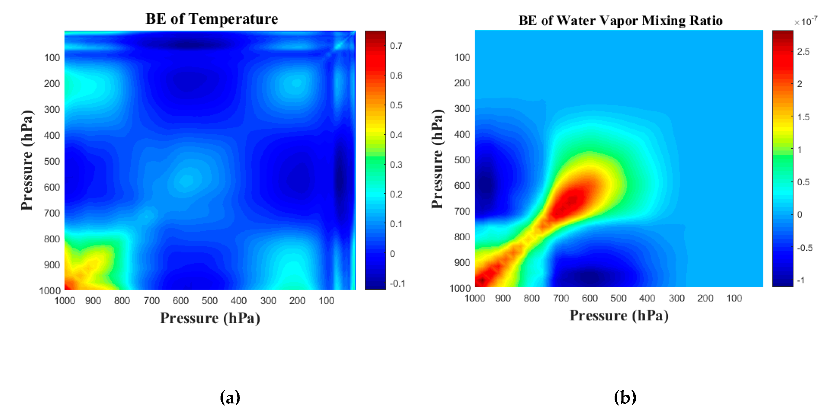
where bij is the background error covariance of the layers i and [33]. To build the background error covariance matrix, the reanalysis data from September–November 2018 were selected as the initial field of the WRF model. The simulation area was from 115°E to 118°E and 38°N to 42°N, covering the Beijing area. The time integration step was set to 24 hours and simulation results were output once per hour. After extracting the 12- and 24-hour prediction fields, the background error covariance was calculated. The final background error covariance matrix is shown in Figure 5.
The values on the diagonal of the temperature background error covariance matrix were large, while on the off-diagonal, the values were basically between −0.1 and 0.2 K2, indicating that the influence between different pressure layers was relatively small. There was a large background error covariance of about 0.5 K2 at 1000 hPa. From 800–1000 hPa, the value decreased continuously. There was also a smaller peak with the value of about 0.2 K2 at 600 hPa. In the upper atmosphere from 500 hPa to 1 hPa, the value of the background error covariance was close to 0. The overall change from the near ground to the top of the atmosphere (1000–1 hPa) initially decreased, then increased, and finally the fluctuation decreased to almost 0. The background error covariance matrix of the water vapor mixing ratio is shown in Figure 6 on the right, which was similar to the background error covariance matrix of the atmospheric temperature. The larger values were concentrated on the diagonal and there were multiple peaks along the diagonal. The first peak value appeared near 1000 hPa with the value of about 0.4 (g/kg)2 and the second peak value appears near 650–700 hPa with the value of 0.4(g/kg)2. Overall, the error mainly concentrated in the range of 500–1000 hPa, while at high altitude, the error covariance was almost 0 (g/kg)2 due to the low water vapor content. Both error matrices had large values near the ground; possible reasons for this include the complexity of land types, elevation, and the heterogeneity of the surface, which may cause the ground parameterization scheme in the WRF model to have more uncertainties, thus leading to more errors near the ground.

3.5. Observation Error Covariance Matrix

Observation errors include measurement errors, forward model errors, and representativeness errors [36]. The measurement errors refer to the noise in the radiation measurement, i.e., the sensitivity of the instrument. Forward model errors mainly include measurement errors of atmospheric parameters, imprecise model descriptions, and errors caused by unmodeled complex physical processes. Representativeness errors come from discretization, which means that even though the real state of atmosphere is continuous, the atmospheric variables input into model are discrete. Observation errors are considered to be independent of each other in different channels; therefore, the observation error covariance matrix can be expressed as a diagonal matrix as shown below:
O   =   ( Y     F ( x ) ) 2 n     1 ,
where O represents an element of the diagonal; Y is the brightness temperature observed using HIRAS; and F(x) represents the brightness temperature calculated using RTTOV, where x is generated from WRF; and n is the number of samples.
The variational assimilation theory assumes that observations are unbiased and Gaussian [15]. However, due to observation errors and model errors, systematic errors often exist in observation fields, which may restrict the full use of observation data [37,38]. Therefore, it is necessary to correct the error of the observation and calculate the covariance of observation error.
First, the mean bias (MB) of the simulated and observed brightness temperature of each channel is calculated as follows:
E   =   ( Y     F ( x ) ) n ,
Then, the element of diagonal R is given as:
O   =   ( Y     F ( x )     E ) 2 n     1 ,
In order to establish the observation error covariance matrix required by the algorithm and evaluate the effect of the observation deviation correction, the data from 29 September 2018, 4 October 2018, and 21 November 2018 was used. The simulation region was also from 115°E to 118°E and 38°N to 42°N. In RTTOV, the number of simulated layers was set to 88 and the simulated air pressure was from 1 to 1000 hPa. The space matching between the simulated brightness temperature and the observed brightness temperature of HIRAS was carried out to calculate the covariance of the observation error before and after correcting the deviation. The error correction effect on the observation errors is depicted in Figure 6.

3.6. Retrieval System Framwork

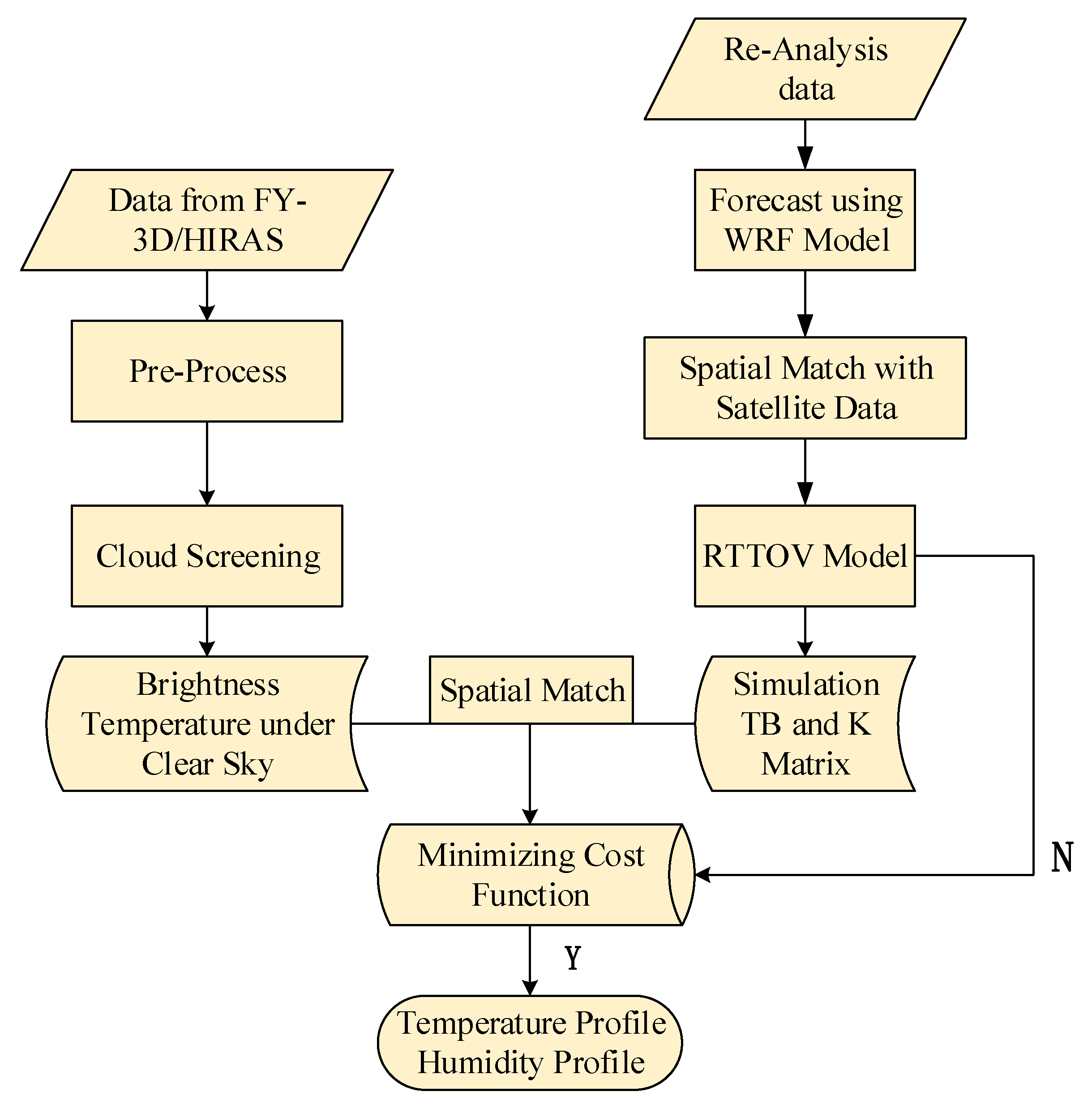
The generic framework of the 1D-VAR for the FY-3D/HIRAS technique implementation is summarized in the flowchart presented in Figure 7. This includes a cloud-screening model to choose the clear-sky pixel, the first guess from the WRF model, a radiative transfer model (RTTOV) as an observation operator, and a minimization method for the cost function. During each retrieval, the satellite data after apodization filtering and quality control is input into the cloud-screening model to obtain the brightness temperature under clear-sky conditions. At the same time, the reanalysis data input into WRF mode are simulated with an integration time step of 6 hours to obtain the initial guess field. After spatial matching with the sensor brightness temperature, RTTOV is run to change the atmospheric state variables into observations and obtain the K matrix. Finally, the Newton nonlinear iteration method is carried out, and the results are evaluated upon completion of each iteration. If convergence cannot be reached, the initial values of the profile are updated and put into RTTOV mode again to run until the final retrieval results are obtained.

4. Case Study

To demonstrate the proposed technique, the region of Beijing has been selected as a case study. It covers a total area of 16,410.54 km2 and its terrain is high in the northwest and low in the southeast. Its climate is typical of the north temperate semi-humid continental monsoon climate, with a high temperature rainy summer, and a cold and dry winter. Horizontal resolutions in the x and y directions are both 5 km. Beijing has two kinds of landforms, namely plain and mountain, which leads to an elevation influence. However, for the convenience of retrieval, such an influence was not considered here. Therefore, according to different pixels, the atmosphere is divided into 88 vertical layers distributed uniformly and extending from 1 hPa to 1000 hPa on the ground.

4.1. Cloud Detection

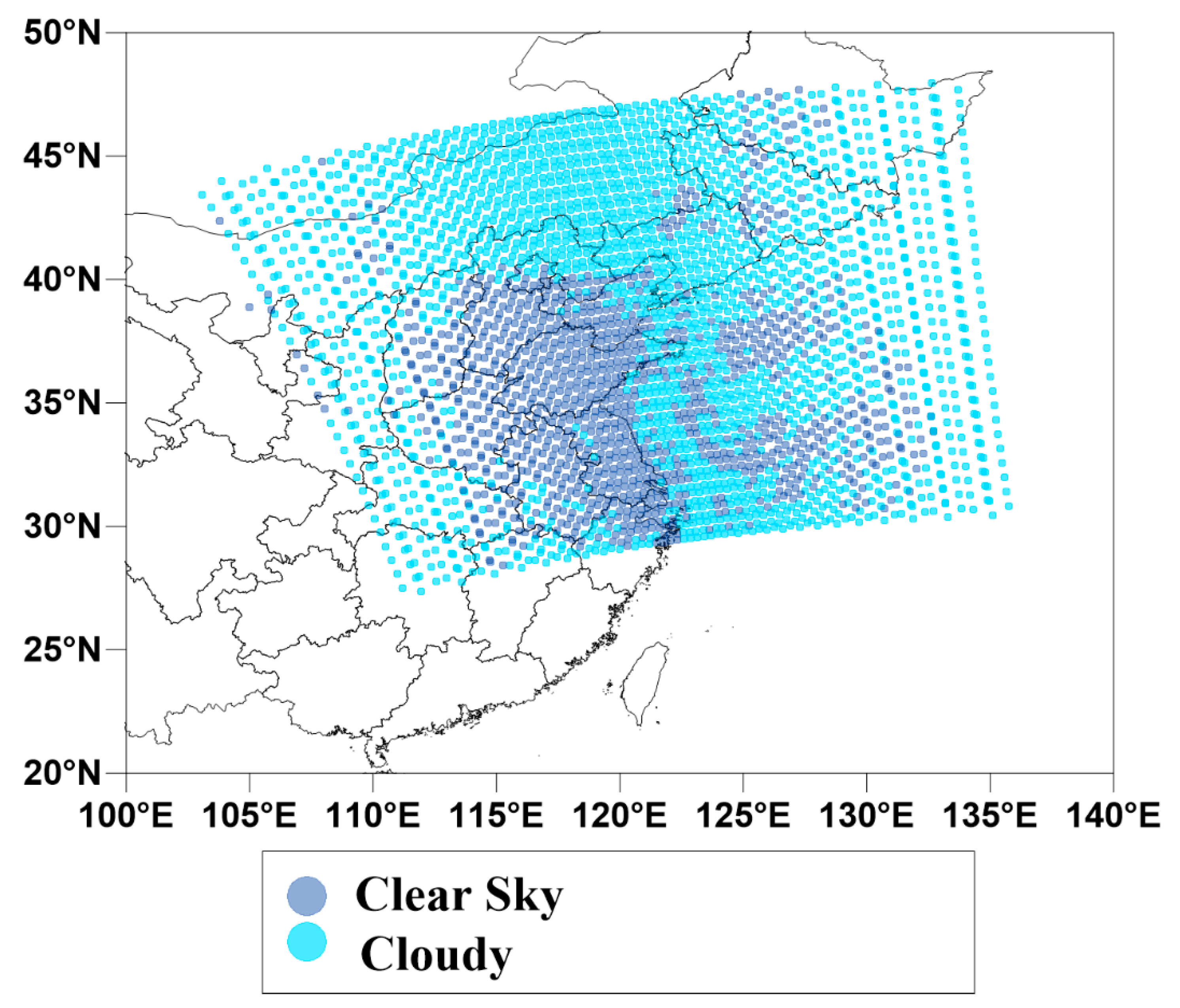
As the detection of the infrared hyperspectral under cloud and rain conditions is not very accurate, these samples need to be removed before retrieving the temperature and humidity profiles. Figure 8 shows an example of the retrievals using a cloud model developed using the GBDT algorithm. The result was based on data from the FY-3D/HIRAS L1 orbit, which passed over China at 05:00 on 12 December 2018. After providing the brightness temperature, solar altitude angle, and satellite observation angle of all cloud detection channels as the input into the established cloud detection model, the model results are presented in the form of judgment marks (cloudy = 1, clear sky = 0). Compared with the cloud products from Himawari-8, the accuracy of the cloud detection model was 86.8%.

4.2. Results of 1D-VAR Retrieval

Taking 11 December 2018 as an example, the orbit of the satellite that passed over Beijing was first selected and the observed brightness temperature of the HIRAS sensor was obtained after data pre-processing and quality control. The initial field for the WRF model was the reanalysis data at 00:00 on 11 December 2018. In the next step, the WRF was simulated for six hours to obtain the background field. Since the selected satellite orbits were from around 05:00 UTC, the simulation result of 05:00 was extracted as the background field of 1D-VAR to become the iterative initial value of minimization process. At the same time, the background field was also selected as input into the RTTOV radiative transfer model to simulate the brightness temperature and obtain the K matrix. These data were input into the established one-dimensional variational retrieval algorithm; the final temperature and humidity profile retrieval results are shown in Figure 9.
To obtain a sufficient sample size to evaluate the retrieval accuracy, 10 days of satellite observation data in July, August, and December 2018 were randomly selected for the retrieval. The samples affected by cloud, rain, and ground elevation were excluded, and the total number of samples left was 294. The accuracies of the retrieved atmospheric profiles were firstly quantified statistically through a comparison with the 06:00 ERA-Interim data, which had a time resolution of 6 hours and spatial resolution of 0.125° × 0.125°. Figure 10 shows the difference between retrieval profiles, background field profiles, and ERA-Interim profiles. The input parameter describing the water vapor in the radiation transfer mode is the water vapor mixing ratio (kg⋅kg−1). To facilitate the comparison of water vapor retrieval results, the water vapor mixing ratio was converted to a relative humidity, and the conversion equation is shown as follows:
e   =   p r 0.622   +   r ,
e s   =   6.1078 exp [ 17.2693882 ( T     273.16 ) T     38 ] ,
RH   =   e e s   ×   100 % .
In Equation (20), e represents the vapor pressure, r represents the water vapor mixing ratio, and p is the pressure. In Equation (21), es represents the saturation vapor pressure, while T represents the temperature. In Equation (22), RH is the relative humidity. As can be seen from Figure 10, both the temperature retrieval results and the background field profile were consistent with the profiles from ERA-Interim; however, the retrieval results were improved compared with the background field near the boundary layer. Regarding other layers, the retrievals were more dependent on the first guess. After the inclusion of satellite observation data, the improvement of the relative humidity profile retrieval was more obvious than that of the temperature profile, and the whole retrieval was relatively close to the standard profile.
The statistical metrics used to evaluate the agreement between the compared datasets included the mean bias (MB), root mean square error (RMSE), mean absolute error (MAE), and the correlation coefficient (R) [39,40,41,42], which are expressed using the following formulas:
MB   =   i = 1 n ( y i     y i ) n ,
MAE   =   i = 1 n | ( y i     y i ) | n ,
RMSE   =   i = 1 n ( y i     y i ) 2 n ,
where n represents the number of samples, y is the true value, and y’ is the retrieval value.
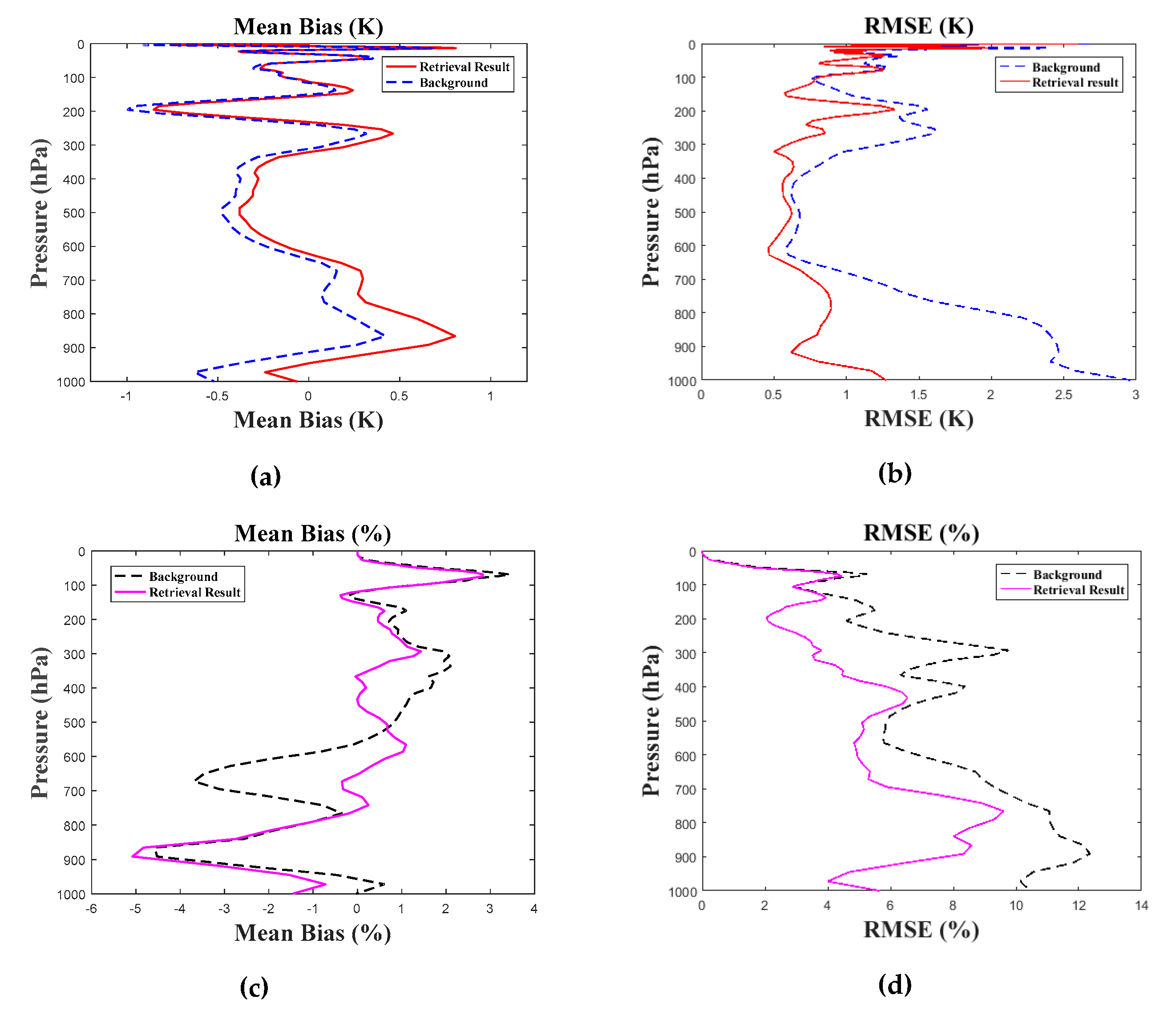
MB, MAE, and RMSE were used to evaluate the accuracy of each layer of the retrieval parameters, while the correlation coefficient shows the degree of correlation between the value of all layers of the retrieval profiles and the corresponding reanalysis data. The results are shown in Figure 11. As can be observed, the MB of the temperature profile was −0.03 K, while the RMSE was 0.95 K, and the correlation coefficient was 0.99. During the temperature retrieval, the bias of the temperature profile fluctuated between −0.8 K and 0.9 K, the MAE was from 0.35 K to 2.27 K, and the RMSE varied between 0.5 K and 2.6 K. The MB, MAE, and RMSE values were reasonable, with a maximum at about 5 hPa. This error possibly resulted from extrapolation for reanalysis data before inputting into the WRF model as it was only up to 100 hPa. Compared with the first guess, the retrieval results were greatly improved near the ground, with an RMSE of 0.88 K, which was a decrease of 1.64 K compared with the first guess, but the retrieval biases at 650–900 hPa were larger. The RMSE of the temperature retrieval profiles was smaller than that of the initial field profiles, which indicates that the profiles were stable after retrieval using a one-dimensional variational algorithm. Meanwhile, the MB of relative humidity profiles was 0.32%, the RMSE was 3.41%, and the correlation coefficient was 0.98. The retrieval deviation of relative humidity in the whole atmosphere was within 6%. The MB of the retrieval results for 150–800 hPa was close to 0, but the value at 900 hPa was larger than the first guess. The RMSE of the whole atmosphere was smaller than the initial field profiles, but the RMSE at 775 hPa was the largest, nearly 10%.
There is a suite of temperature and humidity products generated from infrared hyperspectral sensors, such as AIRS and the Infrared Atmospheric Sounding Interferometer (IASI). The time of IASI passing over Beijing was more than three hours different from the time of HIRAS. Therefore, the time between these two sensors was difficult to match. For this reason, the temperature and humidity profiles obtained from AIRS were employed for further comparisons with retrieval profiles from HIRAS. In this part, HIRAS data were collocated with AIRS for the same period for comparison with the ERA-Interim data with collection criteria of ±1 h in time and ±0.2° in space. The number of collections used to compute the statistics was 109. Regarding temperature, the correlation coefficients of all layers showed in Figure 12a were all above 0.8. These results suggest a consistency of the algorithm results with AIRS’ products, with slight differences above 200 hPa. The temperature consistency was also excellent under 200 hPa, where r was close to 1. As can also be observed, the relative humidity comparisons showed an inconsistency existed near the ground at 400–500 hPa and the tropopause, especially near the surface. Assuming the atmospheric profiles from AIRS to be the standard profiles, as displayed in Figure 12c,d, it can be seen that the MB of the temperature profile was between −2.13 K and 2.93 K, and the MB of all layers was −0.06 K. Notably, the maximum deviation occurred around 1 hPa, and the deviation for 900–10 hPa was within 1 K. The RMSE varied between 0.59 K and 3.70 K, and the maximum RMSE value was also recorded at around 1 hPa. The RMSE value between 900 and 100 hPa was reported to be within 1.5 K. Similarly, the MB of the humidity profile was between −8.31% and 11.57%, and the MB of all layers was 1.70%, with the maximum deviation found at approximately 1000 hPa. The RMSE was between 1.17% and 18.05%, and at the same time, the maximum value was also around 1000 hPa.
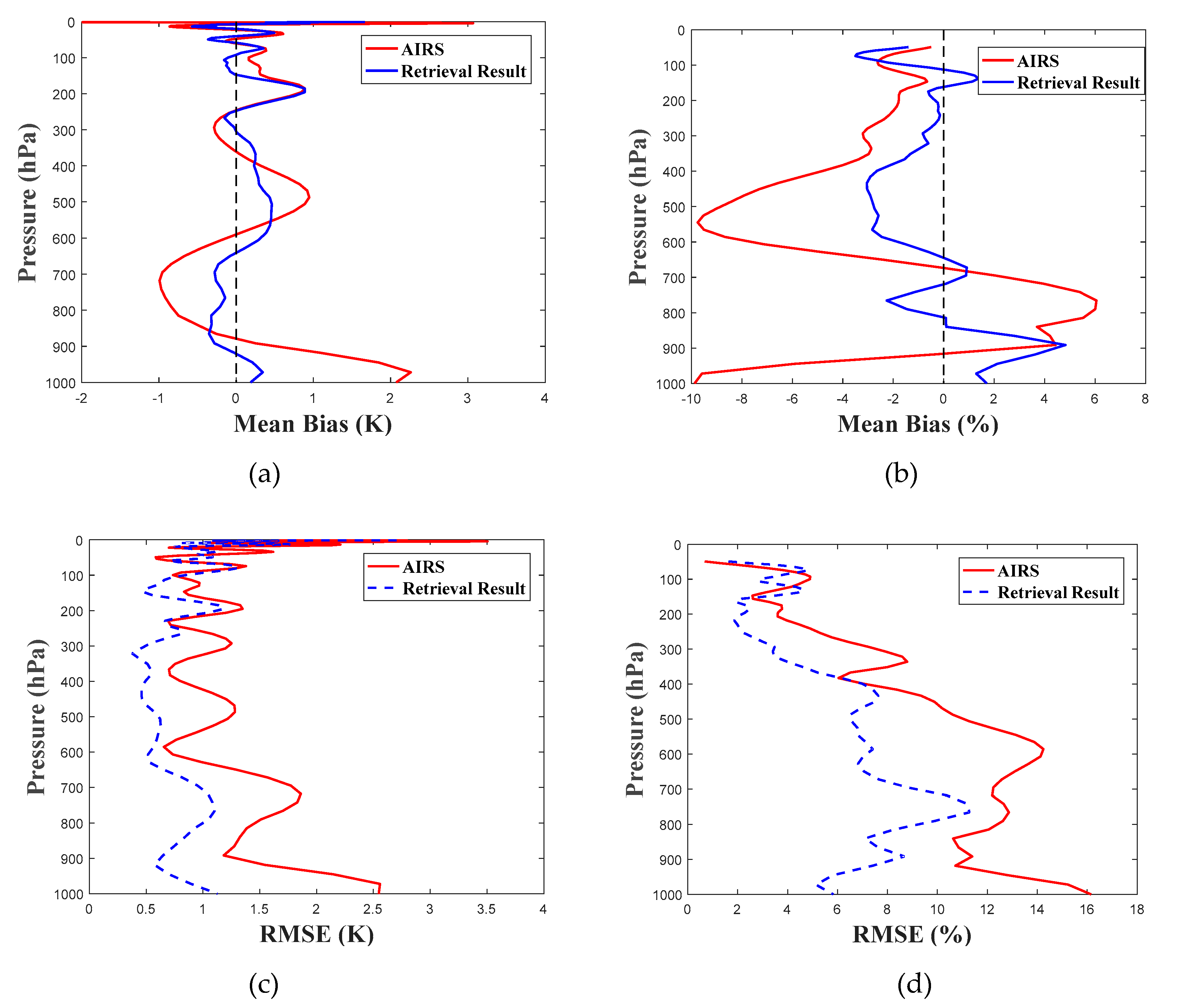
In addition, our results were compared against the AIRS atmospheric profiles and the ERA-Interim data. The ERA-Interim data was assumed to provide the standard profiles, and the results are illustrated in Figure 13. As can be observed, both the temperature and humidity profiles retrieved from HIRAS were close to the ERA-Interim data. The maximum and minimum temperature biases for AIRS were both around 5 hPa, with values of 3.07 K and −1.99 K, respectively. On the other hand, for HIRAS, the maximum and minimum temperature biases were 1.67 K and −0.57 K, respectively. The RMSE of the temperature profile for AIRS varied from 0.58 K to 3.50 K, with the maximum value still near 5 hPa, whereas for HIRAS, the RMSE was from 0.37 K to 2.70 K, and <1.5 K in the troposphere. Comparisons of the relative humidity showed more variable results, but the average biases were all within 10%, which was acceptable. AIRS had a negative humidity bias above 700 hPa. The minimum bias occurred at 550 hPa and near the surface. HIRAS biases among the total atmosphere column were reported to be within 6%. The RMSE for RH was almost the same above the tropopause because little vapor exists there. However, RMSE under 400 hPa varied significantly.

5. Conclusions

This study proposed a one-dimensional variational (1D-VAR) retrieval system to simultaneously retrieve the temperature and humidity profiles under clear-sky conditions. Our technique requires observations acquired from the Fengyun-3D Hyperspectral Infrared Radiation Atmospheric Sounding (HIRAS) satellite and utilizes the Weather Research and Forecast (WRF) model. The accuracy of the proposed technique was evaluated by comparing the temperature profile predictions against the ERA-Interim data using the region of Beijing in China as a case study. Compared with the ERA-Interim 0.125° × 0.125° resolution reanalysis data, the FY-3D/HIRAS temperature and humidity profile products retrieved using this algorithm showed a reasonable consistency, with an RMSE of the temperature within 1 K and humidity within 10%. Compared with the AIRS product, temperature showed a great consistency from 200–1000 hPa, while for relative humidity, the bias and RMSE were larger in the boundary layer. The retrieval results from our system were more consistent with ERA-Interim data than with AIRS’ products. It is worth noting that the background error covariance and observation error covariance established in this algorithm were only applicable to the Beijing region; therefore, the use of this algorithm has certain spatial limitations. Furthermore, it should also be noted that potential error sources in the retrieval process could come from:
  • Time matching: When establishing the observation error covariance matrix, the input of the forward operator adopted the 05:00 simulation results of the WRF, and the corresponding satellite orbit transit time had a deviation of 0–1.5 hours.
  • Space matching: In the inversion algorithm, the satellite pixel and the spatial grid point of the simulated background field from the WRF were not completely spatially matched. The method of spatial matching introduced herein found the closest grid point of the background field within the range of 0.1° with the satellite pixel as the center of longitude and latitude.
  • The forward operator (RTTOV) simulation was not accurate, and there were some errors in the radiation transmission mode. Although some errors were corrected to ensure the Gaussian distribution of the errors in the establishment of the inversion system, such errors could not completely eliminate the effects of simulation errors.
  • The cloud detection model was not accurate. Cloud detection is the premise of temperature and humidity profile inversion. In this inversion system, the accuracy of the cloud detection model was 86.8%, and the clear-sky pixels could not be completely detected.
All in all, our results showed that our proposed technique can be used to obtain retrievals of those parameters in real-time conditions and has a very promising potential for operational implementation in the future. One of its key characteristics is that of expandability. Indeed, different instruments can be added to one-dimensional variational assimilation system if their forward observation operators and error estimates are available. Future work may focus on extending the 1D-VAR method to multi-source sensor integration, such as active and passive remote sensing, ground- based and sky-based remote sensing, etc. This remains to be seen.

Author Contributions

Conceptualization, L.Z. and Y.B.; methodology, L.Z., Y.B., and P.Z.; software, L.Z.; validation, L.Z., Q.L., and F.L.; formal analysis, L.Z.; investigation, G.P.P.; resources, P.Z., Q.L., and F.L.; data curation, Y.W. and D.X.; writing—original draft preparation, L.Z.; writing—review and editing, G.P.P., Y.B., and P.Z.; visualization, Y.W.; supervision, Y.B.; project administration, Y.B. All authors have read and agreed to the published version of the manuscript.

Funding

This study was supported by the National Key Research and Development Program of China (2017YFC1501704, 2018YFC1407200, 2016YFA0600703); National Natural Science Foundation of China (1975046); G.P.P.’s participation was supported financially by the European Union’s Horizon 2020 Marie Skłodowska-Curie Project “ENViSIoN-EO” (grant agreement No 752094).

Acknowledgments

We would like to thank the National Satellite Meteorological Center for sharing FY3D/HIRAS data and giving advice on how to use these data. We also thank the anonymous reviewers for the comments that helped improve our manuscript.

Conflicts of Interest

The authors declare no conflict of interest.

References

  1. Bao, Y.; Cai, X.; Qian, C.; Min, J.; Lu, Q.; Zuo, Q. 0-10 KM Temperature and Humidity Profiles Retrieval from Ground-based Microwave Radiometer. J. Trop. Meteorol. 2018, 24, 243–252. [Google Scholar] [CrossRef]
  2. Li, J.; Li, J.L.; Otkin, J.; Schmit, T.J.; Liu, C.Y. Warning Information in a Preconvection Environment from the Geostationary Advanced Infrared Sounding System—A Simulation Study Using the IHOP Case. J. Appl. Meteorol. Clim. 2011, 50, 776–783. [Google Scholar] [CrossRef]
  3. Menzel, W.P.; Schmit, T.J.; Zhang, P.; Li, J. Satellite-based atmospheric infrared sounder development and applications. B Am. Meteorol. Soc. 2018, 99, 583–603. [Google Scholar] [CrossRef]
  4. Smith, W.L.; Woolf, H.M. The Use of Eigenvectors of Statistical Covariance Matrices for Interpreting Satellite Sounding Radiometer Observations. J. Atmos. Sci. 1976, 33, 1127–1140. [Google Scholar] [CrossRef] [Green Version]
  5. Guan, L.; Huang, A.; Li, J. A Study on Retrieving Atmospheric Profiles from EOS/AIRS Observations. J. Meteorol. Res. Prc. 2005, 19, 112–119. [Google Scholar]
  6. Guan, L. Retrieving Atmospheric Profiles from MODIS/AIRS Observations. I. Eigenvector Regression Algorithms. J. Nanjing Inst. Meteorol. 2006, 6, 756–761. [Google Scholar] [CrossRef]
  7. Liu, H.; Dong, C.H.; Zhang, W.J.; Zhang, P. Retrieval of clear air atmospheric temperature profiles using AIRS observation. Acta Meteorol. Sin. 2006, 66, 513–519. [Google Scholar]
  8. Zhang, J.; Li, Z.L.; Li, J.; Li, J.L. Ensemble Retrieval of Atmospheric Temperature Profiles from AIRS. Adv. Atmos. Sci. 2014, 31, 559–569. [Google Scholar] [CrossRef]
  9. Cabreramercader, C.R.; Staelin, D.H. Passive microwave relative humidity retrievals using feedforward neural networks. IEEE Trans. Geosci. Remote 2002, 33, 1324–1328. [Google Scholar] [CrossRef]
  10. Shi, L. Retrieval of Atmospheric Temperature Profiles from AMSU-A Measurement Using a Neural Network Approach. J. Atmos. Ocean. Technol. 2000, 18, 340–347. [Google Scholar] [CrossRef]
  11. Churnside, J.H.; Stermitz, T.A.; Schroeder, J.A. Temperature Profiling with Neural Network Inversion of Microwave Radiometer Data. J. Atmos. Ocean. Technol. 1994, 11, 105. [Google Scholar] [CrossRef] [Green Version]
  12. Devendra, S.; Bhatia, R.C. Study of temperature and moisture profiles retrieved from microwave and hyperspectral infrared sounder data over Indian regions. Indian Radio Space Phys. 2006, 35, 286–292. [Google Scholar]
  13. Cimini, D.; Hewison, T.J.; Martin, L.; Guldner, J.; Gaffard, C.; Marzano, F.S. Temperature and humidity profile retrievals from ground-based microwave radiometers during TUC. Meteorol. Z. 2006, 15, 45–56. [Google Scholar] [CrossRef]
  14. Hewison, T.J. 1D-VAR Retrieval of Temperature and Humidity Profiles from a Ground-Based Microwave Radiometer. IEEE Trans. Geosci. Remote 2007, 45, 2163–2168. [Google Scholar] [CrossRef]
  15. Mirza, C.R.; Koike, T.; Yang, K.; Graf, T. Retrieval of Atmospheric Integrated Water Vapor and Cloud Liquid Water Content Over the Ocean from Satellite Data Using the 1-D-Var Ice Cloud Microphysics Data Assimilation System (IMDAS). IEEE Trans. Geosci. Remote 2007, 46, 119–129. [Google Scholar] [CrossRef]
  16. Boukabara, S.A.; Garrett, K.; Chen, W.C.; Sanchez, F.I.; Grassotti, C.; Kongoli, C.; Chen, R.Y.; Liu, Q.H.; Yan, B.H.; Weng, F.Z.; et al. MiRS: An all-weather 1DVAR satellite data assimilation and retrieval system. IEEE Trans. Geosci. Remote 2011, 49, 3249–3272. [Google Scholar] [CrossRef]
  17. Li, J.; Zeng, Q.C. Atmospheric infrared remote sensing and its retrieval problems in clear sky: I. Theoretical study. Chin. J. Atmos. Sci. 1997, 21, 1–9. [Google Scholar]
  18. Li, J.; Zeng, Q.C. Atmospheric infrared remote sensing and its retrieval problems in clear sky: II. Research on retrieval test. Chin. J. Atmos. Sci. 1997, 21, 87–95. [Google Scholar]
  19. Liu, Q.H.; Weng, F.Z. One-dimensional variational retrieval algorithm of temperature, water vapor, and cloud water profiles from advanced microwave sounding unit (AMSU). IEEE Trans. Geosci. Remote 2005, 43, 1087–1095. [Google Scholar] [CrossRef]
  20. Duncan, D.I.; Kummerow, C.D. A 1DVAR retrieval applied to GMI: Algorithm description, validation, and sensitivities. J. Geophys. Res. Atmos. 2016, 121, 7415–7429. [Google Scholar] [CrossRef] [Green Version]
  21. Jang, H.S.; Sohn, B.J.; Chun, H.W.; Li, J.; Weisz, E. Improved AIRS temperature and moisture soundings with local a priori information for the 1DVAR method. J. Atmos. Ocean. Technol. 2017, 34, 1083–1095. [Google Scholar] [CrossRef]
  22. Martinet, P.; Cimini, D.; Angelis, F.D.; Canut, G.; Unger, V.; Guillot, R.; Tzanos, D.; Paci, A. Combining ground-based microwave radiometer and the AROME convective scale model through 1DVAR retrievals in complex terrain: An Alpine valley case study. Atmos. Meas. Technol. 2017, 10, 3385–3402. [Google Scholar] [CrossRef] [Green Version]
  23. Yang, J.; Zhang, P.; Lu, N.M.; Yang, Z.D.; Shi, J.M.; Dong, C.H. Improvements on global meteorological observations from the current Fengyun 3 satellites and beyond. Int. J. Digit. Earth 2012, 5, 251–265. [Google Scholar] [CrossRef]
  24. Zhang, P.; Lu, Q.; Hu, X.; Gu, S.; Yang, L.; Min, M.; Chen, L.; Xu, N.; Sun, L.; Bai, W.; et al. Latest Progress of the Chinese Meteorological Satellite Program and Core Data Processing Technologies. Adv. Atmos. Sci. 2019, 36, 1027–1045. [Google Scholar] [CrossRef]
  25. Saunders, R.; Matricardi, M.; Brunel, P. An improved fast radiative transfer model for assimilation of satellite radiance observations. Q. J. R. Meteor. Soc. 1999, 125, 1407–1425. [Google Scholar] [CrossRef]
  26. Saunders, R.; Hocking, J.; Turner, E.; Rayer, P.; Rundle, D.; Brunel, P.; Vidot, J.; Roquet, P.; Matricardi, M.; Geer, A.; et al. An update on the RTTOV fast radiative transfer model (currently at version 12). Geosci. Model Dev. 2018, 11, 2717–2737. [Google Scholar] [CrossRef] [Green Version]
  27. Martinet, P.; Dabas, A.; Donier, J.M.; Doffer, T.; Garrouste, O.; Guillot, R. 1D-Var temperature retrievals from microwave radiometer and convective scale model. Tellus A 2015, 67, 27925. [Google Scholar] [CrossRef] [Green Version]
  28. Guan, Y.H.; Chen, H.; Ren, J.; Zheng, T.W. An Analytical Study on the Differential Equation of Mesoscale Symmetric Instability under Deep Convection. In Proceedings of the International Conference on Applied Mathematics and Mechanics (ICAMM), Bangkok, Thailand, 29–30 October 2016. [Google Scholar] [CrossRef] [Green Version]
  29. Mcnally, A.P.; Watts, P.D. A cloud detection algorithm for high-spectral-resolution infrared sounders. Q. J. R. Meteor. Soc. 2003, 129, 3411–3423. [Google Scholar] [CrossRef]
  30. Natekin, A.; Knoll, A. Gradient boosting machines, a tutorial. Front. Neurorobot. 2013, 7, 21. [Google Scholar] [CrossRef] [Green Version]
  31. Susskind, J.; Barnet, C.D.; Blaisdell, J.M. Retrieval of atmospheric and surface parameters from AIRS/AMSU/HSB data in the presence of clouds. IEEE Trans. Geosci. Remote 2003, 41, 90–409. [Google Scholar] [CrossRef]
  32. Cao, X.Q.; Zhang, W.M.; Song, J.Q.; Zhang, L.L. Modeling Background Error Covariance in Variational Data Assimilation with Wavelet Method. In Proceedings of the Third International Conference on Information & Computing(ICIC), Wuxi, China, 4–6 June 2010. [Google Scholar] [CrossRef]
  33. Deblonde, G.; Garand, L.; Gauthier, P.; Grassotti, C. Assimilation of SSM/I and GOES Humidity Retrievals with a One-Dimensional Variational Analysis Scheme. J. Appl. Meteorol. 1995, 34, 1536–1550. [Google Scholar] [CrossRef] [Green Version]
  34. Parrish, D.F.; Derber, J.C. The National Meteorological Center’s spectral statistical interpolation analysis system. Mon. Weather Rev. 1992, 120, 1747–1763. [Google Scholar] [CrossRef]
  35. Bannister, R.N. Collection of Results on Background Error Covariance Models. DARC Internal Report 7. Reading, UK, 2006. Available online: https://scholar.google.com.tw/scholar?hl=en&as_sdt=0%2C5&q=Collection+of+Results+on+Background+Error+Covariance+Models&btnG= (accessed on 6 January 2020).
  36. Bouttier, F.; Courtier, P. Data assimilation concepts and methods March 1999. Meteorological training course lecture series. Available online: https://scholar.google.com.tw/scholar?hl=en&as_sdt=0%2C5&q=Data+assimilation+concepts+and+methods+March+1999&btnG= (accessed on 6 January 2020).
  37. Auligné, T.; McNally, A.P.; Dee, D.P. Adaptive bias correction for satellite data in a numerical weather prediction system. Q. J. R. Meteor. Soc. 2010, 133, 631–642. [Google Scholar] [CrossRef]
  38. Dee, D.P.; Uppala, S. Variational bias correction of satellite radiance data in the ERA-Interim reanalysis. Q. J. R. Meteor. Soc. 2009, 135, 1830–1841. [Google Scholar] [CrossRef]
  39. Yang, J.; Min, Q. Retrieval of Atmospheric Profiles in the New York State Mesonet Using One-Dimensional Variational Algorithm. J. Geophys. Res. Atmos. 2018, 123, 7563–7575. [Google Scholar] [CrossRef]
  40. Che, Y.; Ma, S.; Xing, F.; Li, S.; Dai, Y. An improvement of the retrieval of temperature and relative humidity profiles from a combination of active and passive remote sensing. Meteorol. Atmos. Phys. 2019, 131, 681–695. [Google Scholar] [CrossRef]
  41. He, Q.; Wang, Z.; He, J. Temperature and humidity profiles retrieving over land using clear sky measurements of microwave humidity-temperature sounder on Chinese FY-3C satellite. In Proceedings of the IEEE International Geoscience and Remote Sensing Symposium (IGARSS), Beijing, China, 10–15 July 2016; pp. 4161–4164. [Google Scholar]
  42. Subrahmanyam, K.V.; Kumar, K.K. Megha-Tropiques/SAPHIR measurements of humidity profiles: Validation with AIRS and global radiosonde network. Atmos. Meas. Technol. 2013, 6, 11405–11437. [Google Scholar] [CrossRef]
Figure 1. Distribution and corresponding ground field map of the HIRAS detector.
Remotesensing 12 00435 g001
Figure 2. The influence of apodization on satellite receiving radiation. From left to right is long wave medium wave 1, and medium wave 2. The black line shows the radiation after apodization, while the red one represents the raw radiation.
Remotesensing 12 00435 g002
Figure 3. (a) The normalized Jacobian of the selected temperature channels and (b) the normalized Jacobian of the selected humidity channels. Different colors represent different channels.
Remotesensing 12 00435 g003
Figure 4. Selected channels used during the process of retrieval. The blue dots represent cloud channels. The red dots represent temperature channels and the magenta dots represents vapor channels.
Remotesensing 12 00435 g004
Figure 5. (a) The temperature background error (BE) covariance matrix of the Beijing region (in units of K2) and (b) the water vapor mixing ratio background error covariance matrix of the Beijing region (in units of (g/kg)2).
Remotesensing 12 00435 g005
Figure 6. (a) The effect of the error correction on temperature and (b) the effect of the error correction on humidity.
Remotesensing 12 00435 g006
Figure 7. The general framework of the 1D-VAR assimilation method proposed herein. RTTOV: Radiative Transfer for TOVS, TB: Brightness Temperature WRF: Weather Research and Forecast.
Remotesensing 12 00435 g007
Figure 8. Cloud detection results for 12December 2018.
Remotesensing 12 00435 g008
Figure 9. Contour map of the one-dimensional variational retrieval results from 11 December 2018: (ad) retrieved temperature profiles and (eh) retrieved humidity profiles. Each black dot represents 92 samples.
Remotesensing 12 00435 g009aRemotesensing 12 00435 g009b
Figure 10. (a) Temperature and (b) humidity profiles based on 294 samples. The blue line represents the profile from the ERA-Interim data, the red line represents the profile through 1D-VAR, and the orange line represents the background field profile.
Remotesensing 12 00435 g010
Figure 11. (a,b) The MB and RMSE of the temperature profile, respectively. (c,d) The MB and RMSE of the humidity profile, respectively. The red solid line represents the comparison between the inversion results and the ERA-Interim data, while the blue dotted line represents the comparison between the background field profile and the ERA-Interim data.
Remotesensing 12 00435 g011
Figure 12. (a) The correlation coefficient between the temperature profiles retrieved from HIRAS and the temperature products from AIRS, (b) the correlation coefficient between the relative humidity profiles retrieved from HIRAS and the relative humidity products from AIRS, (c,d) the bias and RMSE for temperature and humidity, respectively. AIRS products are denoted as the standard profiles.
Remotesensing 12 00435 g012
Figure 13. (a,b) The MB and RMSE of the temperature profile, respectively. (c,d) are the MB and RMSE of the humidity profile, respectively. The red solid line represents the comparison between the AIRS products and the ERA-Interim data, while the blue dotted line represents the comparison between retrieval profiles and the ERA-Interim data.
Remotesensing 12 00435 g013
Table 1. Fengyun-3D Hyperspectral Infrared Radiation Atmospheric Sounding (FY-3D/HIRAS) channel spectral characteristic parameters.
Band NameSpectral Range
(cm−1)
Spectral Resolution
(cm−1)
Sensitivity
(NEΔT@250 K)
Long Wave650–1136
(15.3 μm–8.8 μm)
0.6250.15–0.4 K
Medium Wave 11210–1750
(8.26 μm–5.71 μm)
1.250.1–0.7 K
Medium Wave 22155–2550
(4.64 μm–3.92 μm)
2.50.3–1.2 K