Abstract
Super-resolution (SR) technology has shown great potential for improving the performance of the mapping and classification of multispectral satellite images. However, it is very challenging to solve ill-conditioned problems such as mapping for remote sensing images due to the presence of complicated ground features. In this paper, we address this problem by proposing a super-resolution reconstruction (SRR) mapping method called the mixed sparse representation non-convex high-order total variation (MSR-NCHOTV) method in order to accurately classify multispectral images and refine object classes. Firstly, MSR-NCHOTV is employed to reconstruct high-resolution images from low-resolution time-series images obtained from the Gaofen-4 (GF-4) geostationary orbit satellite. Secondly, a support vector machine (SVM) method was used to classify the results of SRR using the GF-4 geostationary orbit satellite images. Two sets of GF-4 satellite image data were used for experiments, and the MSR-NCHOTV SRR result obtained using these data was compared with the SRR results obtained using the bilinear interpolation (BI), projection onto convex sets (POCS), and iterative back projection (IBP) methods. The sharpness of the SRR results was evaluated using the gray-level variation between adjacent pixels, and the signal-to-noise ratio (SNR) of the SRR results was evaluated by using the measurement of high spatial resolution remote sensing images. For example, compared with the values obtained using the BI method, the average sharpness and SNR of the five bands obtained using the MSR-NCHOTV method were higher by 39.54% and 51.52%, respectively, and the overall accuracy (OA) and Kappa coefficient of the classification results obtained using the MSR-NCHOTV method were higher by 32.20% and 46.14%, respectively. These results showed that the MSR-NCHOTV method can effectively improve image clarity, enrich image texture details, enhance image quality, and improve image classification accuracy. Thus, the effectiveness and feasibility of using the proposed SRR method to improve the classification accuracy of remote sensing images was verified.
1. Introduction
Geostationary orbit remote sensing satellites have the advantages of high temporal resolution and large imaging width, which enables them to continuously cover large areas. Consequently, images from geostationary orbit satellites are frequently utilized in meteorology, environmental protection, fire monitoring, and other remote sensing applications [1,2]. The application of such images is becoming increasingly popular due to continuous worldwide efforts in developing a new generation of geostationary satellite sensors. Therefore, geostationary orbit remote sensing satellites are now producing an unprecedented amount of earth observation data. For example, recently, the new generations of the GOES-R satellite series in North America [3,4], the Himawari-8/9 satellite in Japan [4,5], and the Fengyun-4A (FY-4A) satellite [6,7] and the GF-4 satellite in China [8,9] have been successfully launched, and the MTG-I satellite in Europe is scheduled for launch in 2021 [10]. Images from geostationary orbit remote sensing satellites offer an opportunity to use super-resolution reconstruction (SRR) technology to further improve image spatial resolution and mapping.
It is extremely difficult to obtain high spatial resolution images from geostationary orbit remote sensing satellites due to the limitations of optical imaging payload technology, the physical constraints of the imaging instruments themselves, the high altitude of the satellites, and the large distance to the imaging object (which is dozens of times that of low-earth-orbit satellite images). Spatial resolution is of key importance for the utility of satellite-based earth observing systems [11]. Multispectral satellite images with a high spatial resolution can provide detailed and accurate information for land-use and land-cover mapping [12]. The factors that affect the spatial resolution of multispectral sensors include the orbit altitude, the speed of the platform, the instantaneous field of view, and the revisit cycle. Studies have investigated ways to improve the spatial resolution of images from geostationary orbit remote sensing satellites via post-processing, since it is very difficult to upgrade multiple imaging devices once a satellite has been launched.
Methods for the mapping of remote sensing images include hard classification and soft classification techniques [13]. Traditional hard classification techniques generally cannot effectively classify mixed pixels in land cover. Techniques such as maximum likelihood classification (MLC) [14], support vector machine (SVM) [15], and random forest classifiers (RFC) [16] can all effectively classify mixed pixels by estimating the fractional abundance of land cover classes in each mixed pixel. However, these methods are limited by the distribution in the spatial information of land cover. Research on super-resolution mapping (SRM) has developed rapidly in recent years. SRM is a super-resolution soft classification based on the Markov random field theorem, in which the fractional images are first allocated randomly under computational constraints [17], and the initialized results are then optimized by changing the spatial arrangement of subpixels to gradually approach a certain objective, or via a pixel-swapping optimization algorithm, the neighboring pixel value [18], minimizing the perimeter of the images [19], and geostatistical indicators based on SRM [20] in order to generate a realistic spatial structure on the refined thematic map. Due to the limited performance of the soft classification of low-resolution image datasets, the SRM method has high algorithm complexity and slow operational efficiency. Therefore, artificial intelligence algorithms, such as genetic algorithms [21], particle swarm optimization [22], and sparse algorithms [23,24] have not been fully employed in the processing of images from geostationary orbit multispectral remote sensing satellites.
In this study, the accuracy of mapping based on images from geostationary orbit remote sensing satellites was improved using super-resolution reconstruction (SRR). The employed method is different to the SRM approach in that it can increase the number of informative pixels using the mismatch in ground texture information from image to image. These reconstructed higher spatial resolution images can then be classified without any limitation on the classification techniques adopted. The SRR method has been widely used for the processing of remote sensing satellite images. It includes (1) a frequency-domain method, (2) a combined spatial-domain and frequency-domain method, and (3) a deep-learning-based method. The SRR method is simple to implement and can be implemented in parallel; however, the classification result is poor. The airspace reconstruction method is comprised of the non-uniform sampling interpolation iterative back projection (IBP) method [25], projection onto convex sets (POCS) methods [26], the maximum a posteriori (MAP) algorithm [27], the total variation (TV) algorithm, a convolutional neural network algorithm [28,29], etc. However, although these methods are relatively simple and easy to implement, they are not suitable for the practical classification of satellite images. In recent years, a large number of SRR methods based on sparse representation have been developed. However, in the frequency domain, specific transformations can only provide sparse representation for specific types of input signals, and thus it is difficult to develop a general image sparse representation method. Some researchers are currently working on finding a universal solution to the image ill-posed inverse problem. For example, an overlapping group sparsity total variation (OGSTV) model [30] was used to restore damaged images and was demonstrated to be highly effective in reducing the stairstep effect. Additionally, other researchers proposed a model based on the alternating direction method of multipliers (ADMM) to regularize TV and showed this model to be very effective for removing salt and pepper noise, although not random noise [31]. Meanwhile, the authors proposed an SRR method based on dictionary and sparse representation [32]; however, this method required a relatively large number of training samples.
In this paper, we adopt a novel SRR method called the mixed sparse representation non-convex high-order total variation (MSR-NCHOTV) method to achieve the fine classification of images from geostationary orbit remote sensing satellites. To the best of our knowledge, there has been no previous attempt to formulate a solution for a mixed sparse representation model for such classification. The sparsity of the image spatial domain model and OGSTV and NCHOTV regularizers were employed for the removal of staircase artifacts from geostationary orbit remote sensing satellite images. To effectively handle the subproblems and constraints, we adopted the ADMM algorithm to improve the quality of the reconstruction of sparse signals as well as the computing speed of the SRR algorithm. We used low-resolution GF-4 images of sequential frames obtained from the same scene over a short time to ensure the robustness of the algorithm. We improved the spatial resolution of the images by integrating several multispectral GF-4 images acquired on different dates. Overall, it is shown that compared with a bilinear interpolation (BI) SRR method, the MSR-NCHOTV method obtained a better classification and clustering outcome, both visually and numerically.
The remainder of this paper is organized as follows. In Section 2, the methodology of the MSR-NCHOTV SRR method is briefly reviewed. In Section 3, the experimental data and the pretreatment of GF-4 satellite images are described. In Section 4, the classification results are presented and compared to demonstrate the effectiveness of the proposed method. Finally, conclusions are presented in Section 5.
2. Methodology
2.1. Degradation Model of Remote Sensing Images
GF-4 satellite images are likely to suffer from geometric distortion, blurring, and additional noise. In order to reconstruct the images with increased clarity and higher resolution, it is necessary to eliminate many factors that affect image quality, such as blur, platform drift/jitter, and noise. The degradation model of the original remote sensing image is described by the following mathematical expression [33]:
where is an ideal multispectral dataset obtained by sampling a continuous scene at high resolution. is a low-resolution multispectral image recorded by sensor i. K is the number of low-resolution multispectral images. Mi is a warping matrix which represents geometric distortion brought on by vibration of the satellite platform and air turbulence. Hi is a blur matrix representing the imaging system’s modulation transfer function and radiometric distortion. For example that due to atmospheric scattering and absorption, D is a subsampling matrix reflecting the difference in the expected resolution and the actual resolution of the sensor, and represents additive noise with a Gaussian distribution with zero mean. The goal of SRR is to reconstruct the original high-resolution image u based on a series of low-resolution images. This process is completed through image post-processing for each spectral band. The degradation model is established based on the subsequent inversion of the high-resolution image.
2.2. Mixed Sparse Representation Based on Non-Convex Higher-Order Total Variation
In order to find the ill-conditioned solution of Formula (1) for SRR of remote sensing images, the MSR-NCHOTV method with group sparsity for the SRR model is derived as follows:
where and correspond to the overlapping group sparse regularizer and non-convex norm regularizer, respectively; the parameter () is used to guarantee the non-convexity of the function; the variables λ (λ > 0) and ( > 0) are regularization parameters that control the data fidelity term and the non-convex high-order regularizer, respectively; represents the point components in the image domain during the algorithm iteration; when the normalized image pixel value is less than 0, = 0; when the image pixel value is greater than 1, = 1; ∇ and ∇2 are the first- and second-order gradient difference operators, respectively, assuming periodic boundary conditions for the remote sensing image [34]; denotes weights for the contribution of the image spatial domain model; is a characteristic (indication) function in the interval C = [0, 1024] which is used to restore the pixel value of the image between 0 and 1024. This type of constraint is called a box constraint and has been shown to improve the image quality in image restorations. The characteristic function for the set C is defined as [35]:
In order to solve the constrained separable optimization problem of Formula (2), the ADMM method [31] is employed to convert Formula (2) into the following representation:
The augmented Lagrangian function is defined as follows:
where () is a the penalty parameter or regularization parameter, associated with the quadratic penalty terms and ; the variables μ1, μ2, μ3, and μ4 are the Lagrange multipliers associated with the constraints v = ∇u, w = ∇2u, z = u, and r = s, respectively. The objective is to find the critical point of by alternatively minimizing with respect to r, s, u, v, w, z, μ1, μ2, μ3, and μ4. The ADMM method was used to study the optimal solution of each subproblem step by step. Next, we discuss the optimization strategies to solve each subproblem.
(1) The u-subproblem is a least-squares problem with the following form (Formula (6)). Fixing r, s, v, w, and z, solve for u by:
Formula (6) has the following closed-form solution:
Under periodic boundary conditions for the image u, due to the fact that the matrices KTK, ∇T∇, and (∇2)T∇2 are all block circulant with circulant block [35]. The linear system in Formula (7) can be efficiently solved in the Fourier domain using a 2D fast Fourier transform (FFT).
(2) Fixing r, s, u, w, and z, solve for v. The v-subproblem has the following form:
This v-subproblem is an OGSTV denoising problem [30] where the OGSTV regularizer is defined as follows:
where K is the size of the group. The group size can be seen as a K-sized contagious window starting with index i.
We adopted the majorization–minimization (MM) strategy to solve the OGSTV problem in Formula (8). In each iteration of the MM algorithm, a convex quadratic problem is minimized, yielding a convergent solution to Formula (8).
(3) Fixing r, s, u, v, and z, solve for w. The w-subproblem is as follows:
Formula (10) is a non-convex second-order TV denoising problem. In this study, the iterative reweighted l1 (IRL1) algorithm proposed by [36] was adopted to solve the problem of l1 in each iteration of the IRL1 algorithm. The problem in Formula (10) can be solved by approximating the formula as a weighted l 1 problem as in [37]: For , the solution of Formula (11) via one-dimensional shrinkage is given by:
where ti is given by [35].
where ε is a small positive number to avoid division by zero. Now, the weighted l1 problem in Formula (13) can be solved using the one-dimensional shrinkage operator as follows:
where shrink (·) denotes the one-dimensional shrinkage operator.
(4) Fixing r, s, u, v, and w, solve for z. The z-subproblem reads as follows:
The z-subproblem is a projection which ensures that the pixel value stays in the desired range of [0, 1024] (for 16-bit images) [38]. It has the following closed-form solution. The zk+1-subproblem can be rewritten as
where projC (·) is the projection operator.
(5) Fixing r, u, v, w, and z, solve for s. The s-subproblem has the following form:
The method to solve the s-subproblem is the same as that to solve the w-subproblem, and the specific solution method refers to the w-subproblem, which is a least-squares problem with a closed-form solution (Formula (16)).
(6) Fixing s, u, v, w, and z, solve for r. The r-subproblem has the following form:
which is a simple derivative problem.
(7) By updating the Lagrange multipliers μ1, μ2, μ3, and μ4 has the following form:
For ρ, we used an updating rule proposed by [31] that reduces the number of iterations which are required. The convergence of the iterative solution can be partly guaranteed by the above non-convex ADMM methods. In each iteration, by projecting the residual into each domain, the algorithm maintains a large-amplitude component and sets a small-amplitude coefficient to zero, which conforms to the l1 norm minimization. As the iteration progresses, the residuals become progressively smaller. In each iteration, different types of structural components can be reconstructed in the sparse full variation domain and the image spatial domain, respectively. When a suitable number of iterations is reached, the algorithm terminates. Finally, the SRR image is obtained.
2.3. Classification of Multispectral Images using MSR-NCHOTV
The classification of multispectral remote sensing images has always been a key part of remote sensing research. The accurate recognition and classification of multiple types of image is a challenge in the field of remote sensing.
Due to the low spatial resolution and the large number of mixed pixels in multi-spectral images from geostationary orbit satellites, some targets may be difficult to identify, which complicates image classification. Moreover, the SRR-based classification used in this study is not restricted by features, texture information, or the spatial resolution of images and is applicable to all geostationary orbit remote sensing images. Therefore, we employed the SRR method as the preprocessing step of image classification. Thus, by combining different pieces of high-frequency image information from sequential frames of low-resolution geostationary orbit remote sensing satellites, high-resolution images were reconstructed using the MSR-NCHOTV SRR method, and these high-resolution images were then classified.
2.4. Sub-Voxel-Level Joint Registration Between Image Bands
The GF-4 satellite adopts filter switching technology in its remote sensing imaging system. It has a time delay of several seconds in imaging between multiple spectral bands. Research [39] on the stability of the time interval between different image bands has been performed by selecting different images and 22 targets in sequential frames, which illustrated that the imaging time interval of GF-4 image data in each band was about 7.9 s. The difference in imaging time between spectral bands causes the target to shift between different channels. Additionally, the acquired image has serious geometric deformation and low image quality due to the influence of satellite orbit drift, satellite platform wobble, atmospheric disturbance, and changes in the ground surface. Therefore, a method for the registration of remote sensing images is needed to improve the SRR accuracy of images.
Fine registration between remote sensing image bands is the most important step in completing image SRR. Intensity-based image registration methods tend to have high accuracy but low robustness.
Scale invariant feature transform (SIFT) and speed-up robust feature (SURF) are effective image feature point matching algorithms; however, they are computationally complex, and their real-time performance is poor. Rublee et al. showed that oriented fast and rotated brief (ORB) has strong robustness as well as a high data-processing speed (one order of magnitude faster than that of the SURF algorithm and two orders of magnitude faster than that of the SIFT algorithm) [40,41], which can partially compensate for the poor robustness of the intensity-based registration method [42,43]. This study adopts a sub-voxel-level high-precision image registration algorithm based on a combination of ORB feature extraction and an intensity-based registration method [44,45]. The CUDA programming language was utilized to accelerate the sub-voxel-level high-precision image registration algorithm and meet the registration requirements of GF-4 remote sensing images. The registration process of the algorithm is shown in Figure 1.
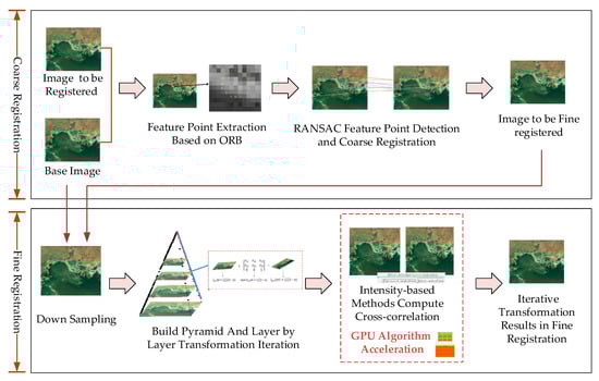
Figure 1.
Workflow of the sub-voxel-level high-precision image registration algorithm based on a combination of oriented fast and rotated brief (ORB) feature extraction and an intensity-based registration process. RANSAC: random sample consensus.
During the image rough registration stage, by selecting the reference image and the image to be registered, the ORB registration algorithm was used for feature extraction. Meanwhile, the random sample consensus (RANSAC) algorithm was used to eliminate the wrong matching points to realize the rough image registration [43]. To ensure the operational efficiency of the algorithm, only a small number of high-precision and evenly distributed matching point pairs need to be selected in the process of feature-point extraction and the elimination of rough imperfections since the ORB registration algorithm mainly realizes rough registration function. After the matching point pairs were obtained, the monography matrix was calculated to generate the rough registration results by image transformation. In the fine registration stage, the base image and coarse image to be fine-registered were sampled, and the image Gaussian pyramid was constructed. The cross-correlation information in the image area was then calculated. Due to the large amount of computation required for this process, a high-speed GPU parallel processing method was adopted to accelerate the algorithm implementation. The image was fine-tuned layer by layer in the Gaussian pyramid of each layer through iterative looping, and the accurate image registration was finally obtained.
3. Experimental Data and Pretreatment
3.1. Experimental Data
This study used image datasets from the GF-4 geostationary orbit remote sensing satellite. This is China’s first high-resolution geostationary orbit optical imaging satellite and the world’s most sophisticated high-resolution geostationary orbit remote sensing satellite. The GF-4 satellite was launched on 29 December 2015 from the Xichang Satellite Launch Center in Sichuan Province, Southwestern China, and is equipped with a CMOS plane array optical remote sensing camera. The GF-4 satellite has a high temporal resolution, high spatial resolution, and large imaging width. It has a ground spatial resolution of 50 m, an image width of 500 × 500 km, an orbital height of 36,000 km, and allows high-frequency, all-weather, continuous, long-term observation of large areas [8,44].
3.2. Research Area
In this study, two sets of 10 consecutive GF-4 satellite image frames with different shooting times and covering different regions were selected. The spatial resolution of these experimental data is 50 m, and the shooting interval is one frame per minute.
Dataset 1 covered the Binhai New area of Tianjin City, covering the intersection between the Shandong Peninsula and the Liaodong Peninsula from 38°40′~39°00′N and 117°20′~118°00′E. The data were acquired at 10:40 a.m. on 24 August 2018. The Binhai New area has 153 km of coastline, a land area of 2270 km2, and a sea area of 3000 km2. The climate characteristics of the area have components of a continental warm temperate zone monsoon climate and a maritime climate.
Dataset 2 was acquired at 09:00 a.m. on 25 June 2016 and covered the Wendeng City district, Weihai City, Shandong Province. The Wendeng City district, located in the east of the Shandong Peninsula from 36°52′~37°23′N and 121°43′~122°19′E, covers a total area of 1645 km2 and has 155.88 km of coastline. The district has a continental monsoon climate with four distinct seasons.
According to the imaging mode of the GF-4 geostationary orbit staring satellite, a pixel window of 1024 × 1024 was selected from each group of images for the study area in order to improve the classification efficiency of the satellite images, as shown in Figure 2.
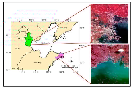
Figure 2.
The two study areas used in this work.
In this study, an SVM classification method was adopted to verify the classification accuracy of the proposed method. In the classification process, high-resolution Google Earth images of the two study areas were used to verify the correctness of the selection of the classification training samples.
3.3. Experimental Process
GF-4 satellite images have a wide coverage, and the region of interest (ROI) varies from frame to frame. In this paper, methods for cutting GF-4 satellite images are divided into manual and automatic methods. In the process of selecting the same ROI area in each GF-4 image frame for cutting, the size of each frame was 10,240 × 10,240 pixels. Although the position of each frame is offset relative to the position of the other frames, the cutting of the ROI area is not affected since each frame is the same size. Firstly, we selected an image frame, annotated the X and Y coordinates of the point in the top left corner of the cutting area, and then entered the length and width of the image to be cut using a cutting algorithm in the Matlab 2019a software (MathWorks, Natick, MA, USA) and the C++ programming language, finally obtaining the required cutting area of the ROI.
Due to the influence of various factors in the satellite remote sensing imaging process, the image acquisition time is inconsistent for each spectral segment. By conducting band registration between Band 1 and Bands 2, 3, 4, and 5, respectively, of the same frame of the GF-4 satellite image, it was found that the difference in pixel values between different bands of each frame of the GF-4 satellite image is one or more pixels, and the difference in spatial resolution is tens to hundreds of meters. The results of the band registration accuracy evaluation of a single frame of a GF-4 satellite image are shown in Table 1.

Table 1.
Results of the band registration accuracy evaluation of a single frame of a Gaofen-4 (GF-4) satellite image.
Pixel offset errors between the bands of the GF-4 satellite greatly reduce the data quality of the GF-4 satellite images, and thus, greatly affect the subsequent processing and application of GF-4 satellite data. Therefore, we adopted a joint registration method based on ORB feature extraction and intensity to improve the accuracy of the SRR. As shown in Figure 3, the red and green double images of the registered image are completely superposed, thus greatly improving the quality of the GF-4 satellite image.
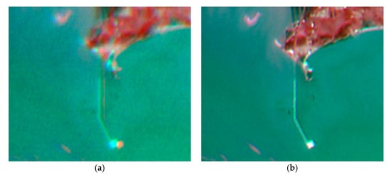
Figure 3.
Comparison of an original GF-4 image (a) and the band-registered image (b).
4. Experimental Results and Analysis
4.1. Evaluation of Image Quality
In order to obtain higher-resolution satellite images, the SRR of GF-4 satellite images was carried out using the MSR-NCHOTV algorithm, which was run using the Ubuntu 16.04 Linux environment. In order to verify the effectiveness of the algorithm, SRR was also carried out on the same GF-4 satellite images using other SRR algorithms, namely BI [24], the POCS method [25], and the IBP method [26], respectively. Image evaluation included subjective evaluation and objective evaluation. The objective evaluation method involved determining the resolution, image sharpness, root-mean-square error, signal-to-noise ratio (SNR), point spread function (PSF), modulation transfer function (MTF), and the classification accuracy of the image super-segmentation results. In this study, the sharpness and SNR of the super-segmented images were used to evaluate the accuracy of the SRR results.
Image sharpness, also known as image average gradient, is obtained by calculating the intensity gradient for every pixel in the image. In this study, the image sharpness was evaluated based on the change in gray level between adjacent pixels following the method proposed by [46]. The higher the image blur value, the lower the image sharpness. The formula for image blur is as follows:
where b_Fhor represents the change in gray level of the neighboring pixel in the horizontal direction, b_Fver represents the change in gray level of the neighboring pixel in the vertical direction, and blurF represents the maximum change in gray level of the neighboring pixels. Firstly, the image was reblurred using a Gaussian filter, and the image quality was then evaluated by calculating the changes in gray level between neighboring pixels before and after reblurring. If the change is large, it indicates that the distortion caused by image blurring is small; otherwise, it indicates that the image distortion is large.
SNR is an important characteristic parameter that is used to evaluate the quality of remote sensing images. It can help data providers or users to better predict image quality and improves their ability to extract information from remote sensing images. The SNR reflects the ratio of signal to noise in the image; the higher the value, the better the quality of the remote sensing image. In this study, the method for the measurement of the SNR of remote sensing images with a high spatial resolution proposed by [47] was used to divide the high spatial resolution remote sensing data into a region with a homogeneous SNR and a region with a heterogeneous SNR. For the homogeneous area, the local standard deviation of the SNR in the small window was calculated by sliding the small window across the whole homogeneous area. All of the local standard deviations were sorted from small to large, and the average value of the largest 90% of the local standard deviations was taken as the estimate of noise level (). For the estimation of the noise level in the inhomogeneous area, each pixel value iteration step of the small window was moved over the inhomogeneous area to calculate the local standard deviation and mean noise level in the small window after each slide. The local standard deviations falling into each subinterval were then sorted, and the average value of the minimum local standard deviation of 10% was taken as the estimate of noise level in this subinterval. The remaining local standard deviation was considered to be caused by the edge, texture, and other features. The image SNR estimated by this method can be expressed by Formula (20):
where S indicates the signal strength and represents the noise level. In order to improve the evaluation accuracy of image SNR, in the SNR estimation process, the size of the small sliding window was set to 10 × 10 pixels.
The results of the SRR were classified using SVM. The classification accuracy was quantitatively evaluated using overall accuracy (OA) and the Kappa coefficient.
4.2. Experiment 1
Experiment 1 used Dataset 1 (see Section 3.2). The area covered by this dataset contains a large amount of buildings and vegetation. The data in this area were reconstructed using the BI, POCS, IBP, and MSR-NCHOTV methods, respectively. As can be seen in the Figure 4, the SRR based on MSR-NCHOTV is superior to the SRR based on the POCS method, completely suppressing block step artifacts without changing the original image information and retaining the edge details. In the SRR based on BI, the image edge is relatively fuzzy, while the SRR based on POCS has serious pixel offset due to registration error and does not consider the prior probability of the image, resulting in an overall sharpening of the image. The subjective effect of reconstruction using IBP is superior to that obtained using the other three algorithms; however, the local details are fuzzy. These results show that the MSR-NCHOTV algorithm proposed in this paper achieves the best SRR of the four studied algorithms.
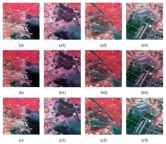
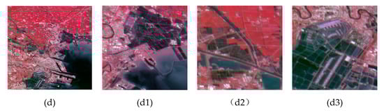
Figure 4.
Results of the super-resolution reconstruction (SRR) for Experiment 1 using the (a) bilinear interpolation (BI), (b) iterative back projection (IBP), (c) projection onto convex sets (POCS), and (d) mixed sparse representation non-convex high-order total variation (MSR-NCHOTV) methods. Panels with the suffixes 1, 2, and 3 show local detail magnifications area of the corresponding panel in the left column.
Using the image quality evaluation metrics of image sharpness and SNR, the results of the four SRR algorithms were objectively analyzed and evaluated. Table 2 and Table 3 show the sharpness and SNR obtained using these four algorithms, respectively. The image blur of each band is largest for the BI algorithm (Table 2). Compared with the POCS method, the IBP method achieved a smaller blur value. The blur value obtained for the MSR-NCHOTV method is the smallest of the four methods, meaning that the image sharpness is the highest, while the image quality is also superior to that obtained using the other three methods. As can be seen in Table 3, the SNR of each band of the BI results is lower than the value obtained using the other three methods, while the SNR of each band of the POCS results is slightly higher than the value obtained using the IBP method. The SNR of each band of the MSR-NCHOTV results is the largest of all the four methods. The results show that the edge and texture information of the complex terrain are improved after SRR using MSR-NCHOTV. Figure 5a,b shows the changes in image sharpness and SNR obtained using the four SRR methods.
Table 2.
Evaluation results for image sharpness.
Table 3.
Evaluation results for image signal-to-noise ratio (SNR).
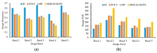
Figure 5.
Image sharpness (a) and SNR (b) for Experiment 1.
The SRR results obtained using the four different methods were classified by SVM. By visual interpretation of high-resolution Google Earth satellite images of the same area, the main types of features in the SRR images were first confirmed, including vegetation, water, buildings, soil, and beach. Then, based on the relative distribution of each object category in the image, 512 sample points were selected from the MSR-NCHOTV SRR image using a stratified random sampling method. The distribution of sample points is shown in Figure 6. The real land-cover categories of these sample points were determined by visual interpretation of the Google Earth images, and the classification accuracy of the various methods was thereby obtained. Figure 7 shows the classification results of the four methods. From the figure, it can be seen that there is more texture information in the MSR-NCHOTV SRR image, especially, edge information of water, roads, etc. As shown in the Table 4, the OA and Kappa coefficient of the MSR-NCHOTV SRR image were 92.75% and 0.91, respectively, which are both significantly higher than those of the SRR images obtained using the three other methods. Table 5 shows the producer’s accuracy (PA) and user’s accuracy (UA) of the SRR images obtained using the four methods for each land-cover category. The results show that the PA and UA of the MSR-NCHOTV SRR image are significantly higher than those of the SRR images obtained using the three other methods, which proves that the MSR-NCHOTV method obtains a higher classification accuracy than these other methods.
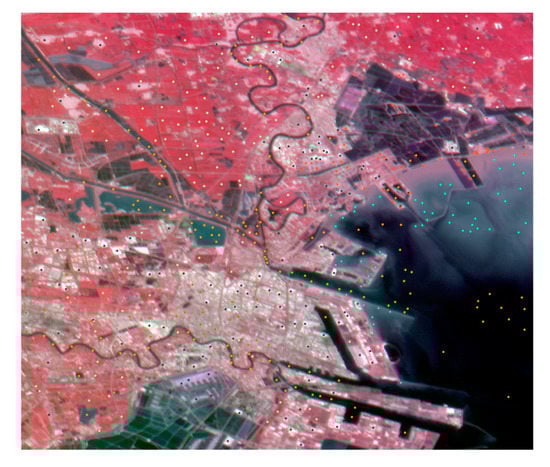
Figure 6.
Distribution of the 512 sample points which were selected from the SRR image for Experiment 1 that was obtained using the proposed MSR-NCHOTV algorithm.
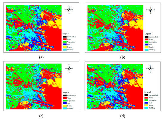
Figure 7.
Classification results for the SRR images for Experiment 1 obtained using (a) BI, (b) POCS, (c) IBP, (d) MSR-NCHOTV.
Table 4.
Results of the overall accuracy (OA) and Kappa coefficient of the four SRR methods.
Table 5.
Results of the producer’s accuracy (PA) and user’s accuracy (UA) of the four SRR methods.
4.3. Experiment 2
Experiment 2 used Dataset 2 (see Section 3.2). In Experiment 2, we used BI, POCS, IBP, and MSR-NCHOTV to perform image SRR, and obtained the images shown in Figure 8. From the figure, it can be seen that the image obtained using BI is fuzzy, and the one obtained using POCS is superior to that obtained using IBP in terms of image clarity and texture details. In the image obtained using MSR-NCHOTV, details of road, vegetation, beach, and other complex texture information are more clearly visible than in the images obtained using the other three methods. Table 6 and Table 7 give quantitative evaluations of the sharpness and SNR, respectively, of the four SRR results. As shown in Table 6, the blur value of the image obtained using the MSR-NCHOTV method is the smallest of all the four methods, and its SNR is the largest of all the four methods (Table 7). Figure 9 shows the sharpness and SNR of the SRR images for separate bands. All the above evidence shows that, of the studied SRR methods, the MSR-NCHOTV method performs the best.
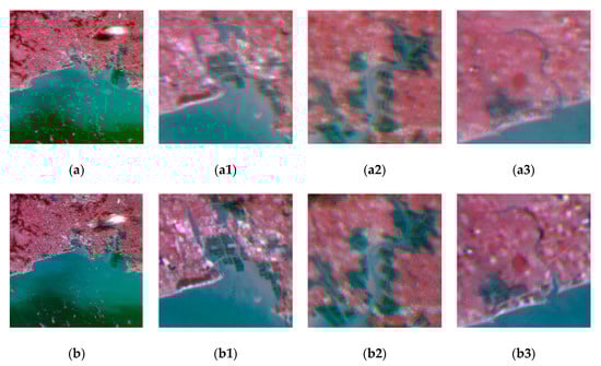
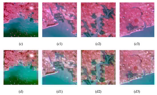
Figure 8.
The SRR images for Experiment 2 obtained using (a) BI, (b) POCS, (c) IBP, (d) MSR-NCHOTV. Panels with the suffixes 1, 2, and 3 show local detail magnifications area of the corresponding panel in the left column.
Table 6.
Evaluation results for image sharpness for Experiment 2.
Table 7.
Evaluation results for image SNR for Experiment 2.
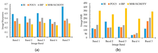
Figure 9.
Image sharpness (a) and SNR (b) for Experiment 2.
Combined with the visual interpretation of Google Earth satellite images, we first identified the main types of land cover in the images, that is, buildings, vegetation, water, farmland, and beach. A stratified random sampling method was used to select 509 sample points. Then, visual interpretation of the Google Earth images was used to determine the real land-cover categories of these sample points. Thus, the classification accuracy of the various methods was obtained. Figure 10 shows the distribution of the sample points. Figure 11a–d shows the mapping results of the four methods. As shown in Figure 11d, in the classification results obtained using the MSR-NCHOTV method, the texture edges and details are more abundant and smoother, respectively, than in the classification results obtained using the three other models. Overall, compared with the images obtained using the three other SRR methods, the image obtained using the MSR-NCHOTV method is visually more similar to the original image. Table 8 shows the results of the OA and Kappa coefficient for the classification of the four SRR images. For the SRR images obtained using the MSR-NCHOTV method image, the OA is 93.3941% and the Kappa coefficient is 0.9121, which are both higher than the values obtained for the classification using the SRR images produced using the three other methods. As shown in Table 9, the PA and UA of buildings, vegetation, water, farmland, and beach for the image obtained using the MSR-NCHOTV method are higher than those obtained using the other three methods.
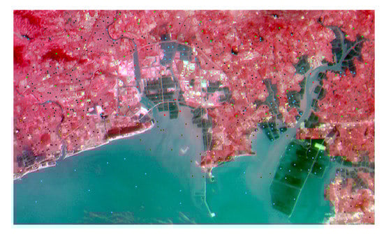
Figure 10.
Distribution of the 509 sample points which were selected from the SRR image for Experiment 2 that was obtained using the proposed MSR-NCHOTV algorithm.
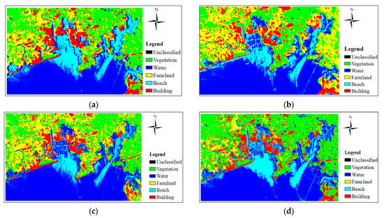
Figure 11.
Classification results for the SRR images for Experiment 2 which were obtained using (a) BI, (b) POCS, (c) IBP, (d) MSR-NCHOTV.
Table 8.
The OA and Kappa coefficient of the classification for Experiment 2 using the SRR images obtained using the four methods.
Table 9.
The PA and UA of the classification obtained using the SRR images for Experiment 2 for each land cover category.
5. Discussion
In this paper, it is shown that the proposed MSR-NCHOTV SRR method can significantly improve the spatial resolution and sharpness of images and provide abundant texture information and detail. Compared with the SRR results obtained using the BI method [24], the sharpness and SNR of the five bands of the GF-4 satellite images obtained using the MSR-NCHOTV SRR method were higher by an average of 39.54% and 51.52%, respectively. Compared with the SRR results obtained using the POCS method [25], the sharpness and SNR of the five bands of the GF-4 satellite images obtained using the MSR-NCHOTV SRR method were higher by an average of 11.86% and 43.63%, respectively. Compared with the SRR results obtained using the IBP method [26], the sharpness and SNR of the five bands of the GF-4 satellite images obtained using the MSR-NCHOTV SRR method were higher by an average of 18.00% and 40.27%, respectively (Table 10).
Table 10.
The percentage improvements in the sharpness and SNR of the SRR image obtained using the MSR-NCHOTV method relative to those of the SRR images obtained using the BI, POCS, and IBP methods.
Table 11 shows a comparison of the OA and Kappa coefficient values of the classification results obtained using the two groups of experimental data, in which the values are expressed as percentage differences relative to the values obtained for the classification based on the image obtained using the BI method [24]. As shown in Table 11, for both experiments, the average OA and Kappa coefficient values obtained using the MSR-NCHOTV method are higher than those obtained using the POCS method [25] and IBP method [26]; compared to the values obtained using the BI method [24], the average values of OA and the Kappa coefficient obtained using the MSR-NCHOTV method are higher by 32.20% and 46.14%, respectively.
Table 11.
The percentage improvements in the OA and Kappa coefficient for the classifications obtained using the POCS, IBP, and MSR-NCHOTV methods, relative to the values obtained using the BI method.
From the above comparative analysis, it can be seen that the sharpness and SNR of the SRR satellite image, and the OA and Kappa coefficient of the classification results, obtained using the MSR-NCHOTV method are all higher than those obtained using the BI, IBP, or POCS methods. The MSR-NCHOTV SRR method has obvious advantages in eliminating step artifacts and maintaining image texture details. Moreover, the method is not restricted by the image category, the image classification method, or the hardware environment. Therefore, the MSR-NCHOTV SRR method has potential as a preprocessing stage for multispectral image classification and can not only improve the spatial resolution of the images but can also generate more abundant information and higher-quality super-resolution images. This method can also be used for the deblurring, feature extraction, fusion, and denoising of remote sensing images. However, the MSR-NCHOTV SRR method is more complicated in parameter selection in the calculation process, and requires multiple iterations in the calculation process, which reduces the operational efficiency of the algorithm. In the future, we will optimize and improve the MSR-NCHOTV SRR method in order to improve the robustness of the algorithm, reduce the computational load, and shorten the operational time, and we will further improve the operational efficiency of the algorithm by using a faster GPU. Additionally, we will also apply this method to the k nearest neighbors (KNN) [48], multi-layer extreme learning machine-based autoencoder (MLELM-AE) [49], and fuzziness and spectral angle mapper-based active learning (FSAM-AL) [50] classification methods, and we will furthermore use the method to achieve the SRR of remote sensing videos.
6. Conclusions
In this study, a method based on the MSR-NCHOTV algorithm was first used to perform SRR of an image from the GF-4 geostationary satellite and to thereby improve the spatial resolution and clarity of the image. Then an SVM method was used to classify the land cover in the reconstructed image. The experimental results show that the overall accuracy and Kappa coefficient of the classification obtained using the SRR image produced using the MSR-NCHOTV method are higher than those obtained using the SRR images produced using the POCS or IBP methods, which proves the feasibility of the proposed MSR-NCHOTV method. This method is not limited to the classification of ground objects nor to the extraction and classification of image information; it can additionally be used in image denoising, image restoration, and other applications. The MSR-NCHOTV method can greatly improve the recognition rate and accuracy of target detection and is of great significance for the use of geostationary orbit satellite data for disaster reduction and prevention, meteorological early warning, and military operations. However, since the implementation of this method is time-consuming, we will attempt to reduce its calculation time and improve its efficiency in the future.
Author Contributions
Conceptualization, X.Y.; methodology, X.Y.; validation, X.Y.; formal analysis, X.Y., F.L.; investigation, X.Y.; writing—original draft preparation, X.Y.; writing-review and editing, X.Y., L.X., X.L.; visualization, M.L.; supervision, N.Z. All authors have read and agreed to the published version of the manuscript.
Funding
This study was supported by the National Key Research and Development Projects (No. 2016YFB0501301) and the National Natural Science Foundation of China (61773383).
Acknowledgments
GF-4 satellite data were provided by the First Institute of Oceanography Ministry of Natural Resources, Qingdao, China.
Conflicts of Interest
The authors declare no conflict of interest.
Abbreviations and Variables
The following abbreviations are used in this manuscript:
| SR | Super-resolution |
| MSR-NCHOTV | Mixed sparse representation non-convex high-order total variation |
| SVM | Support vector machine |
| BI | Bilinear interpolation |
| POCS | Projection onto convex sets |
| IBP | Iterative back projection |
| MLC | Maximum likelihood classification |
| RFC | Random forest classifiers |
| SRM | Super-resolution mapping |
| TV | Total variation |
| OGSTV | Overlapping group sparsity total variation |
| ADMM | Alternating direction method of multipliers |
| yi | Low-resolution multispectral image recorded by sensor i |
| u | Ideal multispectral dataset obtained by sampling a continuous scene at high-resolution |
| D | A subsampling matrix reflecting the difference in the expected resolution and the actual resolution of the sensor |
| Overlapping group sparse regularizer | |
| Denotes weights for the contribution of the image spatial domain model | |
| Characteristic (indication) function | |
| Penalty parameter or regularization parameter | |
| μ | The Lagrange multipliers associated with the constraints |
| FFT | Fourier transform |
| SIFT | Scale invariant feature transform |
| SURF | Speed-up robust feature |
| ORB | Oriented fast and rotated brief |
| RANSAC | Random sample consensus |
| SNR | Signal-to-noise ratio |
| KNN | K nearest neighbors |
| MLELM-AE | Multi-layer extreme learning machine-based autoencoders |
| FSAM-AL | Fuzziness and spectral angle mapper-based active learning |
| OA | Overall accuracy |
References
- Lindsey, D.T.; Nam, S.; Miller, S.D. Tracking oceanic nonlinear internal waves in the Indonesian seas from geostationary orbit. Remote Sens. Environ. 2018, 208, 202–209. [Google Scholar] [CrossRef]
- Fang, L.; Zhan, X.; Schull, M.; Kalluri, S.; Laszlo, I.; Yu, P.; Carter, C.; Hain, C.; Anderson, M. Evapotranspiration Data Product from NESDIS GET-D System Upgraded for GOES-16 ABI Observations. Remote Sens. 2019, 11, 2639. [Google Scholar] [CrossRef]
- Kim, Y.; Hong, S. Deep Learning-Generated Nighttime Reflectance and Daytime Radiance of the Midwave Infrared Band of a Geostationary Satellite. Remote Sens. 2019, 11, 2713. [Google Scholar] [CrossRef]
- He, T.; Zhang, Y.; Liang, S.; Yu, Y.; Wang, D. Developing Land Surface Directional Reflectance and Albedo Products from Geostationary GOES-R and Himawari Data: Theoretical Basis, Operational Implementation, and Validation. Remote Sens. 2019, 11, 2655. [Google Scholar] [CrossRef]
- Bessho, K.; Date, K.; Hayashi, M.; Ikeda, A.; Imai, T. An introduction to Himawari-8/9—Japan’s new-generation geostationary meteorological satellites. J. Meteorol. Soc. Jpn. Ser. II 2016, 94, 151–183. [Google Scholar] [CrossRef]
- Fan, S.; Han, W.; Gao, Z.; Yin, R.; Zheng, Y. Denoising Algorithm for the FY-4A GIIRS Based on Principal Component Analysis. Remote Sens. 2019, 11, 2710. [Google Scholar] [CrossRef]
- Yang, L.; Gao, X.; Li, Z.; Jia, D.; Jiang, J. Nowcasting of Surface Solar Irradiance Using FengYun-4 Satellite Observations over China. Remote Sens. 2019, 11, 1984. [Google Scholar] [CrossRef]
- Zhang, T.; Ren, H.; Qin, Q.; Sun, Y. Snow Cover Monitoring with Chinese Gaofen-4 PMS Imagery and the Restored Snow Index (RSI) Method: Case Studies. Remote Sens. 2018, 10, 1871. [Google Scholar] [CrossRef]
- Chang, X.; He, L. System Noise Removal for Gaofen-4 Area-Array Camera. Remote Sens. 2018, 10, 759. [Google Scholar] [CrossRef]
- Zhang, P.; Lu, Q.; Hu, X.; Gu, S.; Yang, L.; Min, M.; Chen, L.; Xu, N.; Sun, L.; Bai, W.; et al. Latest progress of the Chinese meteorological satellite program and core data processing technologies. Adv. Atmos. Sci. 2019, 36, 1027–1045. [Google Scholar] [CrossRef]
- Tao, Y.; Muller, J.P. Super-Resolution Restoration of MISR Images Using the UCL MAGiGAN System. Remote Sens. 2019, 11, 52. [Google Scholar] [CrossRef]
- Almeida, C.A.; Coutinho, A.C.; Esquerdo, J.C.D.M.; Adami, M.; Venturieri, A.; Diniz, C.G.; Dessay, N.; Durieux, L.; Gomes, A.R. High spatial resolution land use and land cover mapping of the Brazilian Legal Amazon in 2008 using Landsat-5/TM and MODIS data. Acta Amaz. 2016, 46, 291–302. [Google Scholar] [CrossRef]
- Chen, Y.; Ge, Y.; Heuvelink, G.B.; Hu, J.; Jiang, Y. Hybrid constraints of pure and mixed pixels for soft-then-hard super-resolution mapping with multiple shifted images. IEEE J. Sel. Top. Appl. Earth Obs. Remote Sens. 2015, 8, 2040–2052. [Google Scholar] [CrossRef]
- Jain, A.D.; Makris, N.C. Maximum Likelihood Deconvolution of Beamformed Images with Signal-Dependent Speckle Fluctuations from Gaussian Random Fields: With Application to Ocean Acoustic Waveguide Remote Sensing (OAWRS). Remote Sens. 2016, 8, 694. [Google Scholar] [CrossRef]
- Chatziantoniou, A.; Psomiadis, E.; Petropoulos, G.P. Co-Orbital Sentinel 1 and 2 for LULC Mapping with Emphasis on Wetlands in a Mediterranean Setting Based on Machine Learning. Remote Sens. 2017, 9, 1259. [Google Scholar] [CrossRef]
- Zhang, Y.; Cao, G.; Li, X.; Wang, B.; Fu, P. Active Semi-Supervised Random Forest for Hyperspectral Image Classification. Remote Sens. 2019, 11, 2974. [Google Scholar] [CrossRef]
- Li, L.; Chen, Y.; Xu, T.; Liu, R.; Shi, K.; Huang, C. Super-resolution mapping of wetland inundation from remote sensing imagery based on integration of back-propagation neural network and genetic algorithm. Remote. Sens. Environ. 2015, 164, 142–154. [Google Scholar] [CrossRef]
- Butt, A.; Shabbir, R.; Ahmad, S.S.; Aziz, N. Land use change mapping and analysis using Remote Sensing and GIS: A case study of Simly watershed, Islamabad, Pakistan. Egypt. J. Remote Sens. Space Sci. 2015, 18, 251–259. [Google Scholar] [CrossRef]
- De Philippis, G.; Lamboley, J.; Pierre, M.; Velichkov, B. Regularity of minimizers of shape optimization problems involving perimeter. J Math Pure Appl. 2018, 109, 147–181. [Google Scholar] [CrossRef]
- Shi, Z.; Li, P.; Jin, H.; Tian, Y.; Chen, Y.; Zhang, X. Improving Super-Resolution Mapping by Combining Multiple Realizations Obtained Using the Indicator-Geostatistics Based Method. Remote Sens. 2017, 9, 773. [Google Scholar] [CrossRef]
- Tong, X.; Xu, X.; Plaza, A.; Xie, H.; Pan, H.; Cao, W.; Lv, D. A new genetic method for subpixel mapping using hyperspectral images. IEEE J. Sel. Top. Appl. Earth Obs. Remote Sens. 2016, 9, 4480–4491. [Google Scholar] [CrossRef]
- He, D.; Zhong, Y.; Feng, R.; Zhang, L. Spatial-temporal sub-pixel mapping based on swarm intelligence theory. Remote. Sens. 2016, 8, 894. [Google Scholar] [CrossRef]
- Feng, R.; Zhong, Y.; Xu, X.; Zhang, L. Adaptive sparse subpixel mapping with a total variation model for remote sensing imagery. IEEE Trans. Geosci. Remote Sens. 2016, 54, 2855–2872. [Google Scholar] [CrossRef]
- Xu, X.; Tong, X.; Plaza, A.; Zhong, Y.; Zhang, L. Joint sparse sub-pixel mapping model with endmember variability for remotely sensed imagery. Remote Sens. 2017, 9, 15. [Google Scholar] [CrossRef]
- Yoo, J.S.; Kim, J.O. Noise-Robust Iterative Back-Projection. IEEE Trans. Image Process 2019, 29, 1219–1232. [Google Scholar] [CrossRef] [PubMed]
- Zhang, H.; Yang, Z.; Zhang, L.; Shen, H. SRR for multi-angle remote sensing images considering resolution differences. Remote Sens. 2014, 6, 637–657. [Google Scholar] [CrossRef]
- Li, F.; Xin, L.; Guo, Y.; Gao, J.; Jia, X. A framework of mixed sparse representations for remote sensing images. IEEE Trans. Geosci, Remote Sens. 2016, 55, 1210–1221. [Google Scholar] [CrossRef]
- Sun, L.; Zhan, T.; Wu, Z.; Xiao, L.; Jeon, B. Hyperspectral Mixed Denoising via Spectral Difference-Induced Total Variation and Low-Rank Approximation. Remote Sens. 2018, 10, 1956. [Google Scholar] [CrossRef]
- He, Z.; Liu, L. Hyperspectral Image Super-Resolution Inspired by Deep Laplacian Pyramid Network. Remote Sens. 2018, 10, 1939. [Google Scholar] [CrossRef]
- Liu, J.; Huang, T.Z.; Liu, G.; Wang, S.; Lv, X.G. Total variation with overlapping group sparsity for speckle noise reduction. Neurocomputing 2016, 216, 502–513. [Google Scholar] [CrossRef]
- Chen, Y.; Huang, T.Z.; Deng, L.J.; Zhao, X.L. Group sparsity based regularization model for remote sensing image stripe noise removal. Neurocomputing 2017, 267, 95–106. [Google Scholar] [CrossRef]
- Shao, Z.; Wang, L.; Wang, Z.; Deng, J. Remote Sensing Image Super-Resolution Using Sparse Representation and Coupled Sparse Autoencoder. IEEE J. STARS. 2019, 12, 2663–2674. [Google Scholar] [CrossRef]
- Yang, X.; Li, F.; Xin, L.; Zhang, N.; Lu, X.; Xiao, H. Finer scale mapping with super-resolved GF-4 satellite images. In Proceedings of the Image and Signal Processing for Remote Sensing XXV, Strasbourg, France, 9–11 September 2019; Volume 11155, p. 111550A. [Google Scholar]
- Wu, C.; Tai, X.C. Augmented Lagrangian method, dual methods, and split Bregman iteration for ROF, vectorial TV, and high order models. SIAM J. Image Sci. 2010, 3, 300–339. [Google Scholar] [CrossRef]
- Wang, Y.; Yang, J.; Yin, W.; Zhang, Y. A New Alternating Minimization Algorithm for Total Variation Image Reconstruction. SIAM J. Imaging Sci. 2008, 1, 248–272. [Google Scholar] [CrossRef]
- Wu, J.-Y.; Huang, L.-C.; Yang, M.-H.; Chang, L.-H.; Liu, C.-H. Enhanced Noisy Sparse Subspace Clustering via Reweighted L1-Minimization†. In Proceedings of the 2018 IEEE 28th International Workshop on Machine Learning for Signal Processing (MLSP), Aalborg, Denmark, 17–20 September 2018. [Google Scholar]
- Adam, T.; Paramesran, R. Hybrid non-convex second-order total variation with applications to non-blind image deblurring. Signal Image Video Process. 2019, 14, 115–123. [Google Scholar] [CrossRef]
- Condat, L. Discrete total variation: New definition and minimization. SIAM J. Image Sci. 2017, 10, 1258–1290. [Google Scholar] [CrossRef]
- Bao, H.; Li, Z.L.; Chai, F.M.; Yang, H.S. Filter wheel mechanism for optical remote sensor in geostationary orbit. Opt. Precis. Eng. 2015, 23, 11. [Google Scholar]
- Rublee, E.; Rabaud, V.; Konolige, K.; Bradski, G. ORB: An efficient alternative to SIFT or SURF. In Proceedings of the 2011 International Conference on Computer Vision, Barcelona, Spain, 6–13 November 2011. [Google Scholar]
- Tareen, S.A.K.; Saleem, Z. A comparative analysis of sift, surf, kaze, akaze, orb, and brisk. In Proceedings of the 2018 International Conference on Computing, Mathematics and Engineering Technologies (iCoMET), Sukkur, Pakistan, 3–4 March 2018. [Google Scholar]
- Nasihatkon, B.; Fejne, F.; Kahl, F. Globally optimal rigid intensity based registration: A fast fourier domain approach. In Proceedings of the 2016 IEEE Conference on Computer Vision and Pattern Recognition (CVPR), Las Vegas, NV, USA, 27–30 June 2016; pp. 5936–5944. [Google Scholar]
- Acosta, B.M.T.; Heiligenstein, X.; Malandain, G.; Bouthemy, P. Intensity-based matching and registration for 3D correlative microscopy with large discrepancies. In Proceedings of the 2018 IEEE 15th International Symposium on Biomedical Imaging (ISBI 2018), Washington, DC, USA, 4–7 April 2018; pp. 493–496. [Google Scholar]
- Yang, A.; Zhong, B.; Wu, S.; Liu, Q. Radiometric Cross-Calibration of GF-4 in Multispectral Bands. Remote Sens. 2017, 9, 232. [Google Scholar] [CrossRef]
- Hossein-Nejad, Z.; Nasri, M. A-RANSAC: Adaptive random sample consensus method in multimodal retinal image registration. Biomed. Signal Process. 2018, 45, 325–338. [Google Scholar] [CrossRef]
- Crété, F.; Dolmiere, T.; Ladret, P.; Nicolas, M. The blur effect: Perception and estimation with a new no-reference perceptual blur metric. In Proceedings of the Human Vision and Electronic Imaging XII, San Jose, CA, USA, 29 January–1 February 2007; Volume 6492, p. 64920. [Google Scholar]
- Jiehai, C.; Yanchen, B. A method for measuring signal-to-noise ratio of high spatial resolution remote sensing images. Remote Sens. Technol. Appl. 2015, 30, 469–475. [Google Scholar]
- Ahmad, M.; Protasov, S.; Khan, A.M.; Hussain, R.; Khattak, A.M.; Khan, W.A. Fuzziness-based active learning framework to enhance hyperspectral image classification performance for discriminative and generative classifiers. PLoS ONE 2018, 13, e0188996. [Google Scholar] [CrossRef] [PubMed]
- Ahmad, M.; Khan, A.; Mazzara, M.; Distefano, S. Multi-layer Extreme Learning Machine-based Autoencoder for Hyperspectral Image Classification. In Proceedings of the 14th International Conference on Computer Vision Theory and Applications (VISAPP’19), Prague, Czech Republi, 25–27 February 2019; pp. 75–82. [Google Scholar]
- Ahmad, M.; Khan, A.; Khan, A.M.; Mazzara, M.; Distefano, S.; Sohaib, A.; Nibouche, O. Spatial prior fuzziness pool-based interactive classification of hyperspectral images. Remote Sens. 2019, 11, 1136. [Google Scholar] [CrossRef]


© 2020 by the authors. Licensee MDPI, Basel, Switzerland. This article is an open access article distributed under the terms and conditions of the Creative Commons Attribution (CC BY) license (http://creativecommons.org/licenses/by/4.0/).