Extracting Impervious Surface from Aerial Imagery Using Semi-Automatic Sampling and Spectral Stability

Abstract

The quantification of impervious surface through remote sensing provides critical information for urban planning and environmental management. The acquisition of quality reference data and the selection of effective predictor variables are two factors that contribute to the low accuracies of impervious surface in urban remote sensing. A hybrid method was developed to improve the extraction of impervious surface from high-resolution aerial imagery. This method integrates ancillary datasets from OpenStreetMap, National Wetland Inventory, and National Cropland Data to generate training and validation samples in a semi-automatic manner, significantly reducing the effort of visual interpretation and manual labeling. Satellite-derived surface reflectance stability is incorporated to improve the separation of impervious surface from other land cover classes. This method was applied to 1-m National Agriculture Imagery Program (NAIP) imagery of three sites with different levels of land development and data availability. Results indicate improved extractions of impervious surface with user’s accuracies ranging from 69% to 90% and producer’s accuracies from 88% to 95%. The results were compared to the 30-m percent impervious surface data of the National Land Cover Database, demonstrating the potential of this method to validate and complement satellite-derived medium-resolution datasets of urban land cover and land use.

1. Introduction

Over half the Earth’s population now resides in cities [1]. Urbanization inevitably alters hydrologic processes, energy balance, and biological composition, resulting in higher nutrient loads, elevated surface temperature, increased peak flow, and accelerated habitat degradation in many urban areas and watersheds [2,3,4]. A characteristic indicator of urbanization is the increase of impervious surface, a unique land cover class that involves paved roads, sidewalks, parking lots, buildings, and other built structures, through which precipitation does not readily infiltrate into the underlying soil [5]. Understanding the spatiotemporal pattern of impervious surface has important implications for many urban studies on stormwater, heat islands, water quality, ecosystem function, population growth, and community resilience [6,7,8,9,10,11]. The quantification of impervious surface provides critical information to city managers and researchers for a range of issues in urban planning and environmental management [5].

Remote sensing has been used for decades to monitor land cover change and map the growth of impervious surface. This has led to the generation of important databases at national or global scales, such as the National Land Cover Database (NLCD) in the United States [12,13], Coordination of Information on the Environment (CORNIE) land cover inventory in Europe [14], Finer Resolution Observation and Monitoring-Global Land Cover (FROM-GLC) database in China [15], and MODIS Land Cover Type Yearly Global dataset [16]. As these databases are derived from medium-resolution satellite imagery with pixel size ranging from 30 m to 500 m, they have to use multiple urban land cover classes (i.e., low- and high-intensity developed areas) to reflect different levels of impervious surface cover at the scale of a satellite image pixel. High-resolution datasets of impervious surface are not available over large spatial extents, but some studies have utilized meter- or submeter-level aerial imagery to characterize urban landscape. For example, object-based feature extraction and regression tree techniques were applied to National Agriculture Imagery Program (NAIP) orthophotography in Minnesota and led to an overall accuracy of 74% [17]. An algorithm of multiple agent segmentation was applied to analyze NAIP imagery of Rhode Island [18]. More recently, random forest (RF) models were combined with geographic object-based image analysis to generate a 1-m land cover dataset of West Virginia with an overall accuracy of 96.7% [19].

However, reported accuracies for impervious surface were often lower than the accuracies of other land cover classes in supervised classification. An important reason is the acquisition of sufficient and reliable samples that are needed to train a classification model. Studies have shown that increasing the size of training data generally improves classification performance and could have a greater influence than the classification model [19,20]. Collecting a large number of quality samples by field surveys or screen digitalization is very complex, costly, and time consuming [21]. This is exacerbated by the acquisition of independent samples for validation, as using the same data for training and validation could result in optimistically biased accuracy assessments [22]. Another influential factor on the extraction of impervious surface is the selection of variables. Including predictor variables in addition to original image bands generally improves classification performance. These additional predictors include a variety of spectral, textural, and feature geometric indices, derived from the targeted image and sometimes with the support of ancillary datasets [2,19,23,24,25,26,27,28,29]. These measures enhance the signatures of impervious surface across various spatial scales, but they lack the information about the unique temporal behaviors of impervious surface. Although some predictor variables of temporal changes (e.g., phenological features and time series) have been used in studies on vegetation classification [30,31,32], such variables have been rarely included in the extraction of impervious surface.

The goal of this study was to develop a hybrid method for extracting impervious surface from 1-m NAIP imagery. Reference data for training and validation were generated in a semi-automatic scheme that integrated multiple ancillary datasets to minimize human edits. Classification was also improved by analyzing temporal stability of surface reflectance based on a time series of Landsat imagery. We demonstrated this method at three sites in South Texas to address different levels of development intensity and data availability. Furthermore, after the accuracy assessment, the 1-m results of impervious surface were upscaled to 30-m resolution for a comparison to the NLCD percent impervious surface product, demonstrating the potential value of our method to validate and complement this important national land cover database.

2. Materials and Methods

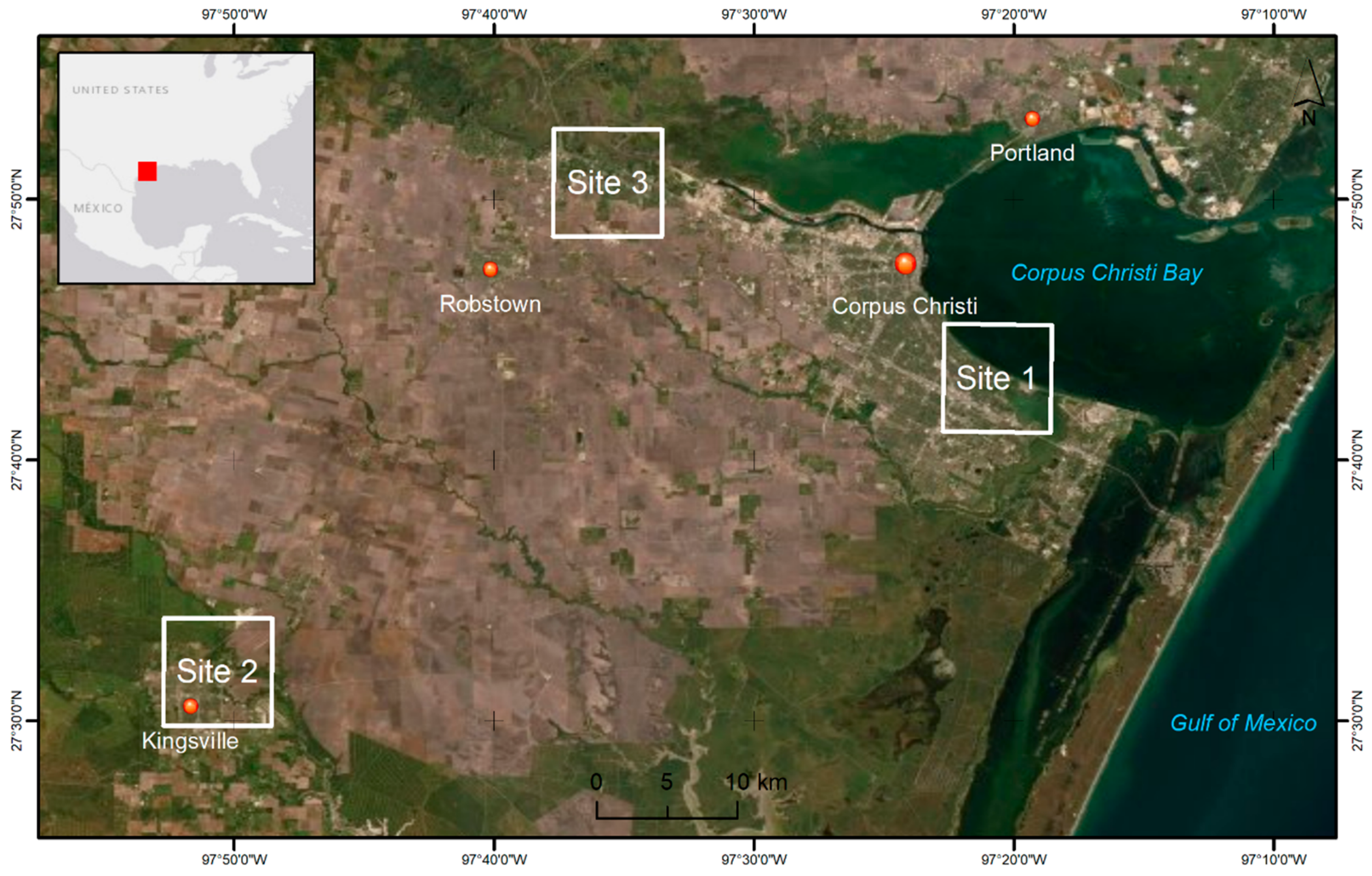
2.1. Study Area and Data

The study area is located in the Corpus Christi-Kingsville metropolitan region in South Texas, United States (Figure 1). This region is a flat coastal plain that faces the Gulf of Mexico. Elevation varies from sea level to 70 m with an average slope of 0.5%. Soils are mainly Victorian clay and Orelia fine sandy loam. According to 2016 NLCD data, the major land cover classes in this area include developed (26%), open water (24%), cultivated crops (15%), hay and pasture (10%), and shrub and scrub (8%). This area has a humid subtropical climate with an average annual precipitation of 805 mm and an average annual temperature of 22.3 °C.

Three sites were selected for this study (Figure 1). Site 1 was in the south region of Corpus Christi, the urban core with a population of 325,733 in 2016. The landscape of this site was dominated by developed land and large areas of coastal water. Site 2 covered the majority of Kingsville, a satellite city with a population of 25,714 in 2016 and surrounded by agricultural land. Site 3 was an industrial zone in north Corpus Christi with a mixture neighborhood of farmland and wetland. Thus, the three sites reflected a gradient of land development: high (Site 1), medium (Site 2), and low (Site 3). They also addressed different conditions of barren land, ranging from limited mixed barren land (Site 1) to abundant single-type barren land (Site 3) and abundant mixed barren land (Site 2). NAIP imagery of these sites consisted of three 1-m multispectral (blue, green, red, and near-infrared) images acquired in May 2016.

Several ancillary datasets were used in this study. Vector datasets of building and roads were downloaded from the database of the OpenStreetMap (OSM) project (www.openstreetmap.org). Built on the concept of volunteered geographic information, the OSM project relies on volunteers to collect information of various built features, collates them on a central database, and distributes free datasets with sound quality [33]. Vector datasets of freshwater and estuarine wetland boundaries were extracted from the National Wetland Inventory (NWI) database of the United States Fish and Wildlife Service. Created through a hierarchical classification framework that utilizes aerial photography, NWI maps are recognized as the most comprehensive wetland maps in the United States [34]. National cropland data were accessed through Google Earth Engine (GEE). This robust raster dataset is created annually by the National Agricultural Statistics Service (NASS) of the United States Department of Agriculture using moderate resolution satellite imagery and extensive agricultural ground truth [35].

We also directly used satellite data, including 9 Landsat-5 TM images, 41 Landsat-7 ETM+ images, and 25 Landsat-8 OLI images, acquired from 2011 and 2016 in the path-26/row-41 scene of the Landsat World Reference System 2. The Landsat data were Level-2 30-m surface reflectance of six bands (blue, green, red, near-infrared, and two shortwave infrared bands). GEE was used to access and process all remote sensing data in this study.

2.2. Sample Generation

We developed a semi-automatic approach to efficiently generate quality training samples for land cover classification (Figure 2). This method uses multiple ancillary datasets to improve the identification of representative pixels for impervious surface, vegetation, water, and barren land.

First, training samples for impervious surface were generated using vector data of buildings and roads extracted from OSM (Figure 3). Building samples were created by buffering building polygons inward by three meters and then calculating the centroids of the buffered polygons. Using the centroids instead of taking random positions within the building polygons reduced the potential disturbance of vegetation around roof edges. Road samples were generated using the vertices of road polylines in OSM. This comprehensive road dataset included a variety of motorway, primary, secondary, residential, and service roads, as well as the lanes in many commercial parking lots. NAIP pixels at the centroids of building polygons and the vertices of road polylines were extracted to establish the pool of samples for impervious surface. The size of this pool would vary with the local availability of OpenStreetMap data. The three sites in this study reflected a gradient of OSM data availability: abundant (Site 1), medium (Site 2), and scarce (Site 3).

Second, a sampling pool of barren land was established to represent both barren wetland (Figure 4) and barren farmland (Figure 5). Barren wetland consists of tidal flats, sand beaches, and sand dunes that are adjacent to natural water bodies. They were first roughly delineated on the NAIP image by overlaying polygons of estuarine and freshwater wetlands extracted from the National Wetland Inventory. Then, barren wetland was identified using masks of NDVI < 0 and NDWI < 0.1, calculated using the green, red, and near-infrared bands of the NAIP image. Barren farmland mainly consists of bare soils in arable lands that are left fallow. Arable lands were first identified using the cultivated areas of the NASS Cropland Data. Then, a threshold of NDVI < 0 was applied to identify pixels without crop cover. We did not attempt to differentiate all non-vegetation patches through NDVI thresholding. The purpose of using an NDVI threshold was to identify representative areas with sufficiently low values of NDVI, which were highly unlikely to be vegetated areas. Samples were randomly generated within these identified areas of barren land.

Third, sampling pools of water and vegetation were established using thresholds of NDVI and NDWI, respectively. The thresholds were calculated based on NDVI and NDWI values of impervious surface samples within the same NAIP image:

$$T_{ND}={\mu }_{imp,ND}+c_{ND}{\sigma }_{imp,NDVI}$$

(1)

where $T_{ND}$ is the threshold of a normalized difference index (i.e., NDVI or NDWI); ${\mu }_{imp,ND}$ and ${\sigma }_{imp,ND}$ denote the mean and standard deviation of this index, respectively, calculated from its values of all impervious surface samples; and $c_{ND}$ is a coefficient with values of 1.0 and 2.0 for NDVI and NDWI, respectively. Pixels with values above the calculated NDVI and NDWI thresholds were determined as vegetation and water samples, respectively.

Last, 600 samples were randomly selected from the pool of impervious surface and 300 samples for each of the other classes (vegetation, water, and barren land), leading to a training dataset of 1500 samples for the targeted NAIP image. Using a large sample size for impervious surface was aligned with the emphasis of this study on separating impervious surface from other land cover classes. If a pool did not contain sufficient samples, all available samples were included. Given the 1-m resolution of NAIP imagery, it was reasonable to assign a single land cover class to each pixel, so we did not consider any mixed land cover classes.

A modified scheme was developed to generate a separate dataset of samples for validation. First, a group of 1500 pixels were randomly selected across the scene of the NAIP image. Second, pixels located within inward-buffered building polygons or outward-buffered road polygons were labeled as impervious surface. Third, pixels with NDVI and NDWI values exceeding the above thresholds (Equation (1)) were labeled as vegetation and water, respectively. Finally, unlabeled points were visually inspected to determine its land cover. In doing so, the effort of manual editing in generating validation samples was significantly reduced.

2.3. Spectral Stability

Spectral stability (in %) describes the variability (standard deviation $\sigma$) of a pixel reflectance ${\rho }_{\lambda }$ relative to the average reflectance $\overline{{\rho }_{\lambda }}$ over the whole time series [36]:

$$T{S}_{\lambda }=100\times \frac{{\sigma }_{\left({\rho }_{\lambda }-\overline{{\rho }_{\lambda }}\right)}}{\overline{{\rho }_{\lambda }}}$$

(2)

This index was calculated using a six-year time series of Landsat imagery that covered the domain of the targeted NAIP image. The time series consisted of Level 2 surface reflectance products from Landsat 5 TM, Landsat 7 ETM+, and Landsat 8 OLI sensors. They are high-level Landsat products generated by the United States Geological Survey (USGS) to eliminate the need for routine reprocessing efforts of geometric, radiometric, and atmospheric corrections [37]. Landsat images with cloud and cloud shadow cover over 50% were excluded. Over the selected satellite images, spectral stability was calculated for each of six bands: Blue, green, red, near-infrared, shortwave infrared 1, and shortwave infrared 2. Details of band characteristics are available on the website of USGS (www.usgs.gov). The generated 30-m spectral stability images were resampled and clipped to align with the 1-m resolution and domain of the targeted NAIP image.

2.4. Classification and Accuracy Assessment

Three types of predictor variables were used in classification: (i) four original NAIP brightness bands (red, green, blue, and near-infrared); (ii) two multispectral indices (NDVI and NDWI) calculated using NAIP brightness bands; and (iii) six bands of spectral stability calculated using the time series of Landsat surface reflectance. This led to a 12-band, 1-m composite image for classification. For each site, a random forest model of 100 trees was trained on GEE using the 1500-sample training dataset and was then applied to the whole NAIP image. Accuracy was assessed using overall accuracy, the kappa statistics, and the class user’s and producer’s accuracies based on the independent 1500-sample validation dataset.

After the 1-m classification results were fully validated, we further compared the results to the NLCD imperviousness product that represents impervious surface as a percentage of developed surface over every 30-m pixel. We first converted our result into a 1-m binary impervious/non-impervious layer. Then, the percent impervious surface was calculated by dividing the number of 1-m impervious pixels by 900 within each of 30-m grids that were aligned with NLCD pixels.

3. Results

3.1. Classification Results

For Sites 1 to 3 (

Table 1. Error matrix of classification results at Site 1 using automatically generated reference data.

		Reference
		Impervious Surface	Vegetation	Water	Barren	Row Total	UA
Classification	Impervious Surface	279	12	8	11	309	90.0%
	Vegetation	2	389	0	0	392	99.5%
	Water	1	0	766	0	766	99.9%
	Barren	12	1	0	17	31	56.7%
	Column Total	277	402	774	28	Overall:	96.2%
	PA	94.9%	96.8%	99.0%	60.7%	Kappa:	0.939

PA = Producer’s accuracy, UA = User’s accuracy.

,

Table 2. Error matrix of classification results at Site 2 using automatically generated reference data.

		Reference
		Impervious Surface	Vegetation	Water	Barren	Row Total	UA
Classification	Impervious Surface	200	31	0	49	280	71.4%
	Vegetation	10	788	0	38	836	94.3%
	Water	1	0	2	0	3	66.7%
	Barren	8	3	0	370	381	97.1%
	Column Total	219	822	2	457	Overall:	91.5%
	PA	91.3%	95.9%	100.0%	81.0%	Kappa:	0.855

and

Table 3. Error matrix of classification results at Site 3 using automatically generated reference data.

		Reference
		Impervious Surface	Vegetation	Water	Barren	Row Total	UA
Classification	Impervious Surface	160	15	4	53	232	69.0%
	Vegetation	17	725	7	32	781	92.8%
	Water	3	0	49	0	52	94.2%
	Barren	2	1	2	430	435	98.9%
	Column Total	182	741	62	515	Overall:	90.6%
	PA	86.8%	97.4%	80.6%	83.3%	Kappa:	0.849

), overall accuracies were 96%, 92%, and 91%, respectively, and kappa values were 0.94, 0.86, and 0.85, respectively. As expected, user’s and producer’s accuracies were higher for vegetation and water relative to the accuracies for impervious surface and barren land. Producer’s accuracies varied from 88% to 95% for impervious surface and from 60% to 84% for barren land. User’s accuracies were more variable, ranging from 69% to 90% for impervious surface and 57% to 99% for barren land. Confusion associated with impervious surface was a primary area of disagreement, accounting for 92%, 63%, and 54% of the classification errors at Sites 1 to 3, respectively. In particular, the classification errors were driven by the confusion between impervious surface and barren land, accounting for over 40% of the classification errors at all sites. As shown in Figure 6, it mainly included the misidentification of impervious surface from various natural bare ground along shorelines (Sites 1 and 3), unpaved rural roads (Sites 2 and 3), and the edges of cropland patches (Site 3). Most of these areas represent a transition zone between a homogeneous landscape feature and its neighboring features that are smaller and more fragmented (i.e., estuary water versus narrow beach zones, and cropland versus rural roads). The resolution mismatch between 1-m NAIP imagery and 30-Landsat imagery was evident in such areas and had an apparent impact on the spectral characteristics of training samples. Another noticeable component of disagreement was the confusion between vegetation and impervious surface in residual areas with low or medium development intensity, accounting for ~25% of the classification errors.

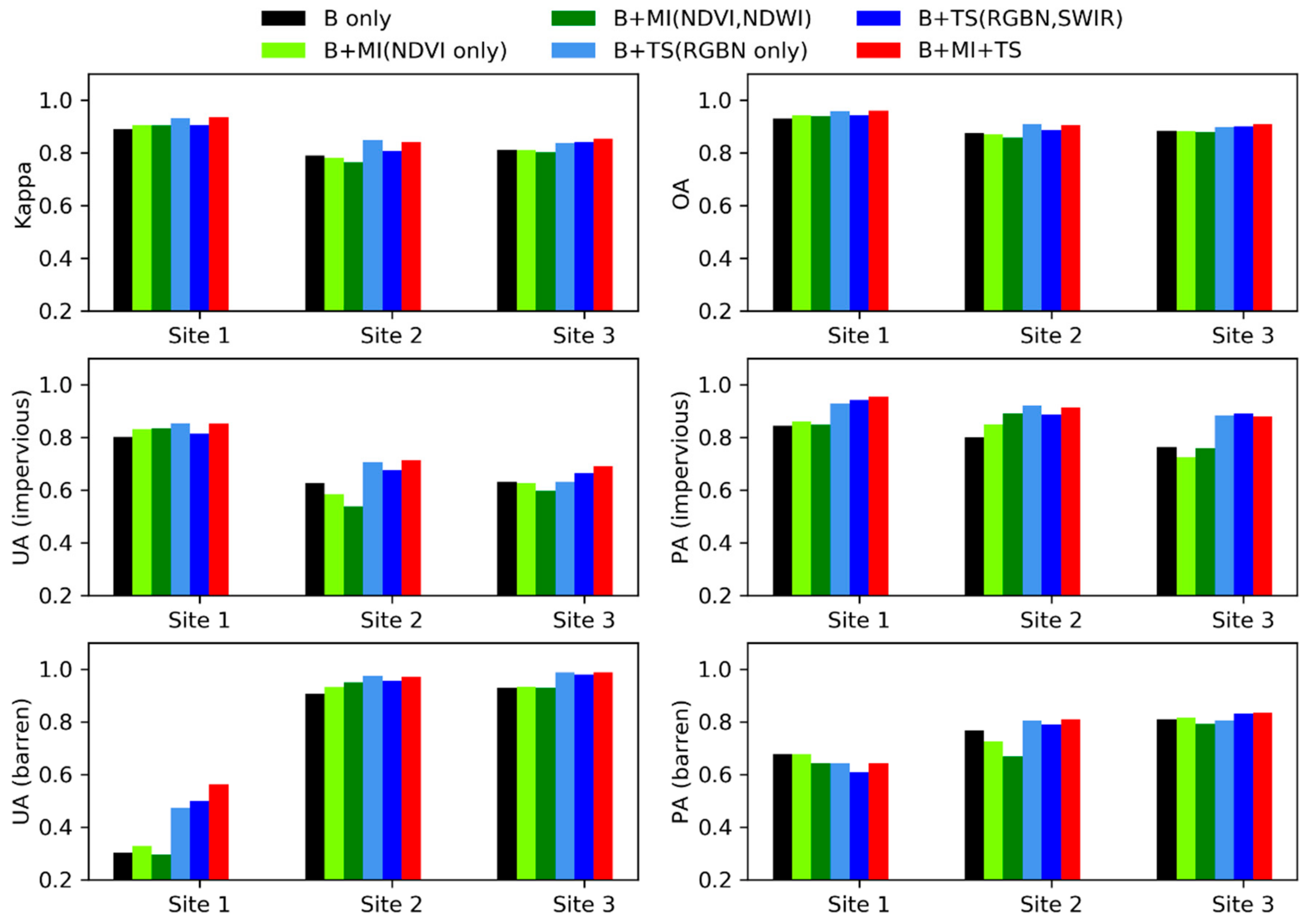
3.2. Selection of Predictor Variables

As shown in Figure 7, including NAIP-derived multispectral indices (i.e., NDVI and NDWI) and Landsat-derived spectral stability led to improved classification accuracies at all three sites, compared to the performance of only using NAIP four-band brightness. Improvements on the identification of impervious surface and barren land were particularly evident. For example, at Site 1, the user’s accuracy of the barren land improved 20% and the producer’s accuracy of impervious surface improved 10%. At Site 3, the user’s accuracy of the barren land improved 5% and the producer’s accuracy of impervious surface improved 13%. This had an important impact on the overall agreement, as the confusion between impervious surface and barren land was the dominant source of classification errors. The results also indicate that including both multispectral indices and spectral stability was more effective than using only one of them. For example, at Site 1, adding multispectral indices alone was better than adding spectral stability alone, but including both further improved the performance.

3.3. Training and Validation Samples

The semi-automatic sampling approach resulted in large training and validation datasets for each site (Figure 8). There were 600, 300, 300, and 300 training samples for impervious surface, water, vegetation, and barren land, respectively. This led to a total of 1500 pixels per NAIP image, i.e., one sample per 35,000 pixels or a high sampling fraction of 0.00286. As expected, the spatial distributions of training samples per class and overall were not homogeneous, as the locations of these samples were confined to scene-specific availability of ancillary data (e.g., OSM building polygons and road polylines) and overall land cover pattern. The validation dataset also consisted of 1500 pixels for each site. Because these pixels were selected using random sampling, the fractions of different land cover categories in the validation dataset reflected the actual land cover composition of the site. The size of validation dataset was deemed sufficient to represent minor land cover categories, e.g., barren ground at Site 1 (2.5%) and water at Site 3 (4.3%). The semi-automatic sampling approach significantly reduced the manual effort of assigning labels to individual pixels. In this study, manual labeling was only needed for 315, 570, and 615 pixels of the validation dataset for Sites 1 to 3, respectively, or on average 17% of the whole 3000-pixel reference dataset per site. To ensure the quality of the reference datasets, visual inspection was performed on all samples that were generated automatically from ancillary data in this study, and no correction was needed for any of them.

Although the semi-automatic sampling approach could generate even larger reference datasets, using more samples did not always lead to enhanced agreement (Figure 9). The performance based on 50 samples per class was quite close to the performance of using 400 samples per class. This indicates that the quality of samples plays a more important role than the quantity of samples in training the random forest models of this study. This is generally consistent with the findings from other studies on the insensitivity of random forest models to the size of training data [19,38].

3.4. NDVI and NDWI Thresholds

The generation of vegetation and water samples relied on the thresholds of NDVI and NDWI, respectively. As shown in Equation (1), the thresholds were determined by: (i) The statistics of index values, calculated from the pool of impervious samples; and (ii) $c_{ND}$, the predefined multiplicative coefficient. Figure 10 and Figure 11 show the responses of classification accuracies to different values of $c_{ND}$, ranging from 0 to 3.0. The increase of $c_{ND}$ for NDVI generally led to decreased producer’s accuracy and increased user’s accuracy (Figure 10). This pattern was more evident for impervious surface than barren land. The default value of 1.0 was associated with high values of overall accuracy and kappa coefficient. In comparison, the change of $c_{ND}$ for NDWI appeared to have limited effect on classification (Figure 11). Exceptions were accuracies of impervious surface at Site 2, where the increased NDWI threshold tended to improve producer’s accuracy and reduce user’s accuracy. The default value of 2.0 for NDWI thresholds yielded good results at all sites.

3.5. Comparison to NLCD data

Figure 12 shows the comparison between the NLCD percent impervious surface and the NAIP-derived percent impervious surface from this study. The NLCD dataset was produced using regressions tree models with predictor variables from Landsat images and ancillary data of nighttime lights and road networks [12,13]. Overall, the two datasets agreed quite well for all three sites, with R² = 0.87, 0.69, and 0.68, respectively. The best agreement occurred at Site 1 due to the high intensity of development and the easy identification of open water. Visual inspection using the original NAIP images (Figure 6a–c) indicates the overestimation of the NLCD data in residential areas mainly due to the misclassification of urban green space as developed land. The NLCD data had a better performance than our results in identifying barren wetland, leading to fewer low-intensity developed areas along shorelines. The confusion with barren land contributed to the overestimation of low-density impervious areas at Site 2 (Figure 10b) and Site 3 (Figure 10c) in our results. Nevertheless, our results suggest a smaller fraction of developed land with medium intensity (i.e., 50%–80% impervious surface cover) compared to the NLCD estimate (Figure 10g–i). This is consistent with the low producer’s accuracy of this class reported by Yang et al. [12].

4. Discussion

Our method addressed two important issues in mapping impervious surface: reference data and selection of predictor variables. Obtaining high-quality reference data is one of the most important factors in achieving an accurate classification and accounts for a major component of time and resource demands [19]. Our method was able to significantly reduce the effort of visual interpretation and manual labeling in the generation of quality samples for training and validation (Figure 8). In the era of big data, the fast expansion of satellite and aerial imagery resources is outpacing the capacity of conventional effort of collecting ground truth through field surveys or on-screen digitalization. Our results suggest that semi-automatic sampling approaches have the potential to fill this gap through efficient uses of existing ancillary data with proven accuracy. The benefit of ancillary data also contributed to the improved inclusion of predictor variables (Figure 7). Through extending variables into the temporal perspective, classification models were able to separate landscape features that were spectrally indifferentiable in a snapshot. This is consistent with findings on the positive effect of including temporal measures in classification [39]. Our method echoes the concept of pseudo-invariant features (PIV) [40,41,42] in radiometric calibration and provides an example of integrating satellite and aerial imagery to enhance the extraction of impervious surface.

The proposed method could contribute to the improved production and assessment of NLCD products and other satellite-derived national land cover data that have played a critical role in a variety of environmental and socioeconomic studies [9,12,13,43]. The landmark assessment by Wickham et al. in 2013 [13] found that user’s accuracies for developed classes in NLCD products increased as the level of urbanization (i.e., percent impervious surface) increased. However, a more recent assessment on NLCD products of 2001–2016 [12] reported an opposite pattern, i.e., increased percent impervious surface was associated with reduced user’s accuracies. Although the overall accuracies in the former study (0.78–0.79) were comparable to that of the later study (0.88–0.90), their conflicting findings in the user’s accuracies of developed land classes indicate a need to improve the consistence of reference data and validation procedure. The agreement of urban classes in NLCD products is generally lower than other land cover classes. A separated assessment on the NLCD imperviousness product has been highly recommended [12]. Wickham et al. [13] suggested that the ideal assessment of NLCD products would require estimation of percent impervious surface for every 30-m pixel based on NAIP imagery, but they had to use a more limited, indirect method because the cost to obtain such ideal reference data was prohibitive. Although a national assessment on the NLCD imperviousness product has not been reported, a recent pilot study in the Chesapeake Bay region has demonstrated the promising value of using NAIP imagery as reference data [44]. The demand of substantial human intervention in generating pixel-level, full-coverage reference data for impervious surface is a major obstacle for the continuous development and validation of NLCD products and similar medium-resolution satellite-derived datasets in other countries.

As indicated in Figure 12, our method could provide an alternative means to verify NLCD products. The quality of samples was ensured by the proven high quality of ancillary datasets. NWI data has already been used as the proxy of ground truth for the validation of satellite-derived land cover products [12], and studies have indicated the trend of incorporating volunteered geographic information data in environmental remote sensing [45,46,47,48]. As our approach is built on GEE and uses publicly available ancillary datasets, it can be easily applied to the validation of NLCD products for other regions. This method provides an efficient, comprehensive, and transferrable way to evaluate the quality of NLCD land cover and imperviousness products. It is feasible to plan for a full validation of NLCD products at the national level using this method, but that would require the technical support of GEE to upgrade the storage and computation capacity that are available for regular users. Those issues are irrelevant to our methodology and are thus beyond of the scope of this paper.

5. Conclusions

A hybrid remote sensing method was developed to improve the extraction of impervious surface from aerial imagery. This method took advantage of multiple ancillary datasets to accelerate the acquisition of reference data and incorporated satellite-derived spectral stability to enhance the signature of impervious surface. This method was applied to three Texas sites with different levels of land development and availability of ancillary data. Results indicate satisfactory separation of impervious surface from barren land, vegetation, and water, with user’s accuracies ranging from 69% to 90% and producer’s accuracies from 88% to 95%. This method was able to significantly reduce the effort of visual interpretation and manual labeling in the generation of quality samples for training and validation. Including measures of spectral stability as predictor variables led to improved classification performance. The comparison of our results to the NLCD percent impervious cover product at the 30-m level indicates the value of this method as an efficient, comprehensive means to validate and complement satellite-derived medium-resolution datasets of urban land cover and land use at regional or national scales.

References

1. WHO. Global Report on Urban Health: Equitable, Healthier Cities for Sustainable Development; World Health Organization: Geneva, Switzerland, 2016. [Google Scholar]
2. Sexton, J.O.; Song, X.P.; Huang, C.; Channan, S.; Baker, M.E.; Townshend, J.R. Urban growth of the Washington, D.C.—Baltimore, MD metropolitan region from 1984 to 2010 by annual, Landsat-based estimates of impervious cover. Remote Sens. Environ. 2013, 129, 42–53. [Google Scholar] [CrossRef]
3. Paul, M.J.; Meyer, J.L. Streams in the urban landscape. Annu. Rev. Ecol. Syst. 2001, 32, 333–365. [Google Scholar] [CrossRef]
4. Arnold, C.L.; Gibbons, C.J. Impervious surface coverage—The emergence of a key environmental indicator. J. Am. Plan. Assoc. 1996, 62, 243–258. [Google Scholar] [CrossRef]
5. Weng, Q. Remote sensing of impervious surfaces in the urban areas: Requirements, methods, and trends. Remote Sens. Environ. 2012, 117, 34–49. [Google Scholar] [CrossRef]
6. Mignot, E.; Paquier, A.; Haider, S. Modeling floods in a dense urban area using 2D shallow water equations. J. Hydrol. 2006, 327, 186–199. [Google Scholar] [CrossRef] [Green Version]
7. Meyer, J.L.; Paul, M.J.; Taulbee, W.K. Stream ecosystem function in urbanizing landscapes. J. N. Am. Benthol. Soc. 2005, 24, 602–612. [Google Scholar] [CrossRef]
8. Lu, D.S.; Weng, Q.H.; Li, G.Y. Residential population estimation using a remote sensing derived impervious surface approach. Int. J. Remote Sens. 2006, 27, 3553–3570. [Google Scholar] [CrossRef]
9. Imhoff, M.L.; Zhang, P.; Wolfe, R.E.; Bounoua, L. Remote sensing of the urban heat island effect across biomes in the continental USA. Remote Sens. Environ. 2010, 114, 504–513. [Google Scholar] [CrossRef] [Green Version]
10. Gobel, P.; Dierkes, C.; Coldewey, W.C. Storm water runoff concentration matrix for urban areas. J. Contam. Hydrol. 2007, 91, 26–42. [Google Scholar] [CrossRef] [PubMed]
11. Brabec, E.; Schulte, S.; Richards, P.L. Impervious surfaces and water quality: A review of current literature and its implications for watershed planning. J. Plan. Lit. 2002, 16, 499–514. [Google Scholar] [CrossRef]
12. Yang, L.; Jin, S.; Danielson, P.; Homer, C.; Gass, L.; Bender, S.M.; Case, A.; Costello, C.; Dewitz, J.; Fry, J.; et al. A new generation of the United States National Land Cover Database: Requirements, research priorities, design, and implementation strategies. ISPRS J. Photogramm. Remote Sens. 2018, 146, 108–123. [Google Scholar] [CrossRef]
13. Wickham, J.D.; Stehman, S.V.; Gass, L.; Dewitz, J.; Fry, J.A.; Wade, T.G. Accuracy assessment of NLCD 2006 land cover and impervious surface. Remote Sens. Environ. 2013, 130, 294–304. [Google Scholar] [CrossRef]
14. Cole, B.; Smith, G.; Balzter, H. Acceleration and fragmentation of CORINE land cover changes in the United Kingdom from 2006–2012 detected by Copernicus IMAGE2012 satellite data. Int. J. Appl. Earth Obs. Geoinf. 2018, 73, 107–122. [Google Scholar] [CrossRef]
15. Yu, L.; Wang, J.; Li, X.; Li, C.; Zhao, Y.; Gong, P. A multi-resolution global land cover dataset through multisource data aggregation. Sci. China-Earth Sci. 2014, 57, 2317–2329. [Google Scholar] [CrossRef]
16. Broxton, P.D.; Zeng, X.B.; Sulla-Menashe, D.; Troch, P.A. A Global Land Cover Climatology Using MODIS Data. J. Appl. Meteorol. Clim. 2014, 53, 1593–1605. [Google Scholar] [CrossRef]
17. Nagel, P.; Yuan, F. High-resolution Land Cover and Impervious Surface Classifications in the Twin Cities Metropolitan Area with NAIP Imagery. Photogramm. Eng. Remote Sens. 2016, 82, 63–71. [Google Scholar] [CrossRef]
18. Zhou, Y.Y.; Wang, Y.Q. Extraction of impervious, surface areas from high spatial resolution imagery by multiple agent segmentation and classification. Photogramm. Eng. Remote Sens. 2008, 74, 857–868. [Google Scholar] [CrossRef] [Green Version]
19. Maxwell, A.E.; Strager, M.P.; Warner, T.A.; Ramezan, C.A.; Morgan, A.N.; Pauley, C.E. Large-Area, High Spatial Resolution Land Cover Mapping Using Random Forests, GEOBIA, and NAIP Orthophotography: Findings and Recommendations. Remote Sens. 2019, 11, 1409. [Google Scholar] [CrossRef] [Green Version]
20. Huang, C.; Davis, L.S.; Townshend, J.R.G. An assessment of support vector machines for land cover classification. Int. J. Remote Sens. 2002, 23, 725–749. [Google Scholar] [CrossRef]
21. Maxwell, A.E.; Warner, T.A.; Fang, F. Implementation of machine-learning classification in remote sensing: An applied review. Int. J. Remote Sens. 2018, 39, 2784–2817. [Google Scholar] [CrossRef] [Green Version]
22. Stehman, S.V.; Foody, G.M. Key issues in rigorous accuracy assessment of land cover products. Remote Sens. Environ. 2019, 231. [Google Scholar] [CrossRef]
23. Piyoosh, A.K.; Ghosh, S.K. Semi-automatic mapping of anthropogenic impervious surfaces in an urban/suburban area using Landsat 8 satellite data. GIScience Remote Sens. 2017, 54, 471–494. [Google Scholar] [CrossRef]
24. Hu, X.F.; Weng, Q.H. Impervious surface area extraction from IKONOS imagery using an object-based fuzzy method. Geocarto Int. 2011, 26, 3–20. [Google Scholar] [CrossRef]
25. Wang, J.; Song, J.W.; Chen, M.Q.; Yang, Z. Road network extraction: A neural-dynamic framework based on deep learning and a finite state machine. Int. J. Remote Sens. 2015, 36, 3144–3169. [Google Scholar] [CrossRef]
26. Kuang, W.; Chi, W.; Lu, D.; Dou, Y. A comparative analysis of megacity expansions in China and the U.S.: Patterns, rates and driving forces. Landsc. Urban Plan. 2014, 132, 121–135. [Google Scholar] [CrossRef]
27. Hamedianfar, A.; Shafri, H.Z.M.; Mansor, S.; Ahmad, N. Improving detailed rule-based feature extraction of urban areas from WorldView-2 image and lidar data. Int. J. Remote Sens. 2014, 35, 1876–1899. [Google Scholar] [CrossRef]
28. Da Silva, V.S.; Salami, G.; Da Silva, M.I.O.; Silva, E.A.; Monteiro Junior, J.J.; Alba, E. Methodological evaluation of vegetation indexes in land use and land cover (LULC) classification. Geol. Ecol. Landsc. 2019, 1–11. [Google Scholar] [CrossRef]
29. Faour, G.; Mhawej, M.; Nasrallah, A. Global trends analysis of the main vegetation types throughout the past four decades. Appl. Geogr. 2018, 97, 184–195. [Google Scholar] [CrossRef]
30. Jia, K.; Liang, S.; Wei, X.; Yao, Y.; Su, Y.; Jiang, B.; Wang, X. Land Cover Classification of Landsat Data with Phenological Features Extracted from Time Series MODIS NDVI Data. Remote Sens. 2014, 6, 11518–11532. [Google Scholar] [CrossRef] [Green Version]
31. Nasrallah, A.; Baghdadi, N.; Mhawej, M.; Faour, G.; Darwish, T.; Belhouchette, H.; Darwich, S. A Novel Approach for Mapping Wheat Areas Using High Resolution Sentinel-2 Images. Sensors 2018, 18, 2089. [Google Scholar] [CrossRef] [Green Version]
32. Shao, Y.; Lunetta, R.S.; Wheeler, B.; Iiames, J.S.; Campbell, J.B. An evaluation of time-series smoothing algorithms for land-cover classifications using MODIS-NDVI multi-temporal data. Remote Sens. Environ. 2016, 174, 258–265. [Google Scholar] [CrossRef]
33. Haklay, M. How good is volunteered geographical information? A comparative study of OpenStreetMap and Ordnance Survey datasets. Environ. Plan. B 2010, 37, 682–703. [Google Scholar] [CrossRef] [Green Version]
34. Matthews, J.W.; Skultety, D.; Zercher, B.; Ward, M.P.; Benson, T.J. Field Verification of Original and Updated National Wetlands Inventory Maps in three Metropolitan Areas in Illinois, USA. Wetlands 2016, 36, 1155–1165. [Google Scholar] [CrossRef]
35. Homer, C.; Dewitz, J.; Yang, L.; Jin, S.; Danielson, P.; Xian, G.; Coulston, J.; Herold, N.; Wickham, J.; Megown, K. Completion of the 2011 National Land Cover Database for the Conterminous United States—Representing a Decade of Land Cover Change Information. Photogramm. Eng. Remote Sens. 2015, 81, 345–354. [Google Scholar] [CrossRef]
36. Bacour, C.; Briottet, X.; Bréon, F.M.; Viallefont-Robinet, F.; Bouvet, M. Revisiting Pseudo Invariant Calibration Sites (PICS) Over Sand Deserts for Vicarious Calibration of Optical Imagers at 20 km and 100 km Scales. Remote Sens. 2019, 11. [Google Scholar] [CrossRef] [Green Version]
37. Young, N.E.; Anderson, R.S.; Chignell, S.M.; Vorster, A.G.; Lawrence, R.; Evangelista, P.H. A survival guide to Landsat preprocessing. Ecology 2017, 98, 920–932. [Google Scholar] [CrossRef] [Green Version]
38. Rodriguez-Galiano, V.F.; Ghimire, B.; Rogan, J.; Chica-Olmo, M.; Rigol-Sanchez, J.P. An assessment of the effectiveness of a random forest classifier for land-cover classification. ISPRS J. Photogramm. Remote Sens. 2012, 67, 93–104. [Google Scholar] [CrossRef]
39. Johnson, D.M. Using the Landsat archive to map crop cover history across the United States. Remote Sens. Environ. 2019, 232, 111286. [Google Scholar] [CrossRef]
40. Zhang, H.; Zimba, P.V.; Nzewi, E.U. A New Pseudoinvariant Near-Infrared Threshold Method for Relative Radiometric Correction of Aerial Imagery. Remote Sens. 2019, 11. [Google Scholar] [CrossRef] [Green Version]
41. Traganos, D.; Poursanidis, D.; Aggarwal, B.; Chrysoulakis, N.; Reinartz, P. Estimating Satellite-Derived Bathymetry (SDB) with the Google Earth Engine and Sentinel-2. Remote Sens. 2018, 10. [Google Scholar] [CrossRef] [Green Version]
42. Small, C. Multitemporal analysis of urban reflectance. Remote Sens. Environ. 2002, 81, 427–442. [Google Scholar] [CrossRef]
43. Singh, K.K.; Madden, M.; Gray, J.; Meentemeyer, R.K. The managed clearing: An overlooked land-cover type in urbanizing regions? PLoS ONE 2018, 13, e0192822. [Google Scholar] [CrossRef] [PubMed] [Green Version]
44. Wickham, J.; Herold, N.; Stehman, S.V.; Homer, C.G.; Xian, G.; Claggett, P. Accuracy assessment of NLCD 2011 impervious cover data for the Chesapeake Bay region, USA. ISPRS J. Photogramm. Remote Sens. 2018, 146, 151–160. [Google Scholar] [CrossRef] [PubMed]
45. Stehman, S.V.; Fonte, C.C.; Foody, G.M.; See, L. Using volunteered geographic information (VGI) in design-based statistical inference for area estimation and accuracy assessment of land cover. Remote Sens. Environ. 2018, 212, 47–59. [Google Scholar] [CrossRef] [Green Version]
46. Viana, C.M.; Encalada, L.; Rocha, J. The value of OpenStreetMap Historical Contributions as a Source of Sampling Data for Multi-temporal Land Use/Cover Maps. ISPRS Int. J. Geo-Inf. 2019, 8. [Google Scholar] [CrossRef] [Green Version]
47. Kaiser, P.; Wegner, J.D.; Lucchi, A.; Jaggi, M.; Hofmann, T.; Schindler, K. Learning Aerial Image Segmentation From Online Maps. IEEE Trans. Geosci. Remote Sens. 2017, 55, 6054–6068. [Google Scholar] [CrossRef]
48. Forget, Y.; Linard, C.; Gilbert, M. Supervised Classification of Built-Up Areas in Sub-Saharan African Cities Using Landsat Imagery and OpenStreetMap. Remote Sens. 2018, 10. [Google Scholar] [CrossRef] [Green Version]
Figure 1. Study area in South Texas, United States.
Remotesensing 12 00506 g001
Figure 2. Flowchart of the generation of training samples using ancillary datasets (green parallelograms). OSM, NASS, and NWI denote OpenStreetMap, National Agricultural Statistics Service, and National Wetland Inventory databases, respectively.
Remotesensing 12 00506 g002
Figure 3. Extracting training samples of impervious surface based on (a) NAIP imagery and (b) OpenStreetMap vector data.
Remotesensing 12 00506 g003
Figure 4. Extracting training samples of barren wetland using three criteria: (a) located within the wetland areas of the NWI dataset, (b) NDWI values < 0.1, and (c) NDVI values < 0. Subplot (d) shows the identified areas of barren wetland and the samples (circles) randomly generated within them.
Remotesensing 12 00506 g004
Figure 5. Extracting training samples of barren farmland using two criteria: (a) Located within the cultivated areas of the USDA Cropland Layer, and (b) NDVI values < 0. Subplot (c) shows the identified areas of barren farmland and the samples (circles) randomly generated within them.
Remotesensing 12 00506 g005
Figure 6. NAIP images and classification results of Site 1 (a,d), Site 2 (b,e), and Site 3 (c,f).
Remotesensing 12 00506 g006
Figure 7. Effect of predictor variables on classification accuracies. In the legend, B, MI, and TS denote brightness, multispectral indices, and temporal spectral stability, respectively. In the y-axis labels of subplots, OA, UA, and PA denote overall accuracy, user’s accuracy, and producer’s accuracy, respectively.
Remotesensing 12 00506 g007
Figure 8. Training samples (ac) and validation samples (df) of the study sites.
Remotesensing 12 00506 g008
Figure 9. Effects of the number of training samples per category on classification accuracies.
Remotesensing 12 00506 g009
Figure 10. Effects of the NDVI threshold on classification accuracies.
Remotesensing 12 00506 g010
Figure 11. Effects of the NDWI threshold on classification accuracies.
Remotesensing 12 00506 g011
Figure 12. Estimates of percent impervious surface by this study (ac) and the NLCD product (df). Subplots (gi) compare the histograms of the two estimates.
Remotesensing 12 00506 g012