1. Introduction
Identifying, characterizing, and mapping land cover is essential for earth system modelling and natural resources planning [
1,
2]. Land cover data establishes the baseline for environmental monitoring (e.g., biogeochemical cycling, sustainable land use, biodiversity loss) and thematic mapping [
3]. Satellite remote sensing has long been used as an ideal technology for land cover mapping and monitoring due to its ability to provide synoptic coverage and repetitive observations over large geographical area in a cost-effective and nearly real-time manner [
4,
5]. While multispectral image data from a single date suffers high level of spectral confusion or spectral similarity between different cover types, multi-temporal data sets, which are more accessible to the remote sensing community because of the advent of cloud-computing [
6] and resources like Google Earth Engine [
7], have proved to be more effective and accurate for vegetation discrimination and classification [
8,
9,
10]. With both spectral and temporal profiles incorporated, time series and their derivations such as vegetation indices (VIs) and further derived vegetation phenological parameters greatly enrich available information for vegetation identification. Thus recently more efforts have been focused on multi-temporal images for land cover mapping [
11].
Among all the VIs, the most commonly used are the normalized difference vegetation index (NDVI) [
12,
13,
14] and the enhanced vegetation index (EVI) [
14,
15,
16,
17,
18,
19]. They are have demonstrated effectiveness to indicate vegetation status and growing phases, and their multi-temporal data are widely applied to land cover classification [
13], agricultural monitoring [
9], and change detection [
20]. However, with only two or three spectral bands used, NDVI and EVI may discard some valuable information or unique characteristics of a certain vegetation at some growing seasons, which means that the most widely used NDVI or EVI may not be the optimal feature for multi-temporal vegetation identification, especially when multiple vegetation types are to be classified simultaneously [
21]. Apart from UNVI and EVI, many other VIs have been proposed and compared in many application scenarios, such as estimation of green leaf area index (LAI) and canopy chlorophyll density [
22,
23]. However, no published study has explored the different performances of different VI time series for land cover mapping, so there may exist other vegetation indices that may outperform NDVI and EVI.
The universal normalized vegetation index (UNVI), established by Zhang et al. [
24], has several advantages over other VIs. UNVI utilizes the information from all observed bands. Expressed as a function of the UPDM (universal pattern decomposition method) coefficients that are sensor-independent, UNVI allows direct comparisons using data from various sources [
24]. Liu et al. [
25] used four VIs including UNVI to describe variations of urban land surface temperature (LST), and UNVI shows the best correlation with LST variations. Jiao et al. [
26] demonstrated that the vegetation condition index (VCI) based on UNVI has stronger correlations with long-term in situ drought indices than NDVI-derived VCI, which means UNVI has considerable potential for drought monitoring [
26]. UNVI has also been applied to estimate chlorophyll content of winter wheat, and demonstrates the best accuracy and stability compared with NDVI and triangle vegetation index (TVI) [
23,
27]. For LAI estimation, UNVI has a higher saturation point than NDVI and EVI, and is more sensitive to a wider range of vegetation dynamics [
23]. These previous studies demonstrate that UNVI is more effective than several commonly used VIs in some certain application scenarios. Therefore, we believe that UNVI is a worth exploring index. However, the performance of UNVI multi-temporal profiles for vegetation discrimination remains unknown.
Therefore, the main objective of this study is to evaluate the vegetation discrimination ability of UNVI time series, and four other VIs were employed for comparison, including NDVI, EVI, TVI, and tasseled cap transformation greenness (TCG). To accomplish this, we designed two comparative experiments: the first one is to analyze class separabilities of specific vegetation types using the UNVI time series and other four VIs data; the second one is to compare the vegetation classification accuracies using the features of these VI temporal profiles and the derived phenological parameters.
3. Methods
The overall procedure for evaluation of vegetation discrimination ability of UNVI time series is shown in
Figure 3. The Landsat 8 surface reflectance data were first preprocessed to obtain noise-free VI time series, and GCC land cover data was downsampled to make it consistent with the Landsat data. Then two comparative experiments, separability analysis and random forest classification, were conducted.
For the downloaded multi-temporal Landsat 8 images, in order to eliminate noisy observations, pixels contaminated by clouds, cloud shadows, and snow were firstly masked according to the quality assessment (QA) bands that were delivered along with surface reflectance bands. UNVI and the other four VIs of the whole year were calculated using the formulas listed in
Table 1. However, the gaps masked by QA band result in missing data along the temporal profile, which may influence the profile reconstruction, so shape-preserving piecewise cubic spline interpolation was used to fill these temporal gaps. In order to eliminate the fluctuations and noises arising primarily from sensor system, atmospheric constituents and surface anisotropy [
38,
39,
40], the temporal profiles of the five VIs were then reconstructed by Savitzky–Golay (SG) filter with a window size of 4.
For the land cover data from GCC, the spatial resolution was downsampled to 30 m, and the pixels were exactly snapped to the Landsat 8 raster images. Considering the widespread small patches and complex distribution of different vegetation types, we applied a morphological operator “erosion” with a structuring element sized 1×1 pixel to each vegetation type to remove all patches’ outermost pixels which are probably mixed ones. The numbers of pixels and area percentage covering the five major vegetation are listed in
Table 3.
Based on the smoothed VIs time series and GCC land cover reference data, we designed two comparative experiments to evaluate the ability of multi-temporal UNVI to distinguish different vegetation. The first one was separability analysis of UNVI and other VIs for the five major vegetation classes. The pixels of each class used for separability calculation were manually selected from large patches in conjunction with Google Earth images to ensure the purity, reliability and distribution uniformity of these pixels. Totally, the amounts of selected pixels were 1821 for crops, 1902 for broadleaf forest, 1134 for coniferous forest, 2374 for deciduous shrub, and 849 for grass, as listed in
Table 3. The second experiment was the comparison of classification performance using different VIs time series and their corresponding phenological parameters as feature sets for the random forest classifier. More details of these two experiments are described below.
3.1. Separability Analysis
The purpose of separability analysis was to evaluate the separability of UNVI time series for different vegetation classes. Separability of each pair in all classes can be quantitatively measured by average distance between the pairwise class density distributions or histograms [
41] of VI values. Three indicators were commonly used: the separability index (SI) [
42,
43,
44,
45], the transformed divergence (TD) [
46,
47] and the Jeffries-Matusita distance (JM distance) [
10,
17,
36,
46]. SI between two classes is defined as the difference between the VI means normalized by the sum of the VI standard deviations. The difference of the means reflects the inter-class variability, while the sum of the standard deviations represents the intra-class variability. The limitation of SI is that when the means of the two classes are equal, SI will always be zero and cannot accurately reflect the separability [
41]. SI can only measure the separability in a one-dimensional feature space such as an individual time point [
45,
48]; thus it cannot meet the needs of our study to calculate the separability of multi-temporal VIs. Compared with TD, JM distance was suggested more reliable in separability measurements [
49], and also more suitable for less homogeneous major classes [
41]. So we chose JM distance to indicate the separability between each pair of vegetation types.
The JM distance is calculated as [
50]:
where
B is the Bhattacharyya distance:
where, for classes
i and
j,
is the mean vector of reflectance values, and
is the variance-covariance matrix. The JM distance ranges from 0 (completely inseparable) to 2 (completely separable), with a larger value indicating a higher degree of separability between the two classes. In this study, the JM distance was calculated for the ten possible combinations of the five vegetation classes with single and multiple temporal UNVI and NDVI, EVI, TVI, TCG.
3.2. Vegetation Classification
To ascertain the ability of the UNVI time series to distinguish the five major classes in Chaoyang prefecture, we further conducted a classification comparison with other four VIs using random forest (RF) method. RF is an ensemble learning algorithm that operates by constructing a multitude of decision trees (without pruning) from random selected training samples and features and deciding the final class based on the majority of votes from all the trees made [
51]. RF is superior to many other classifiers because of its fast training speed, easy parameterization, high accuracy, and noise insensitivity [
15]. RF has been extensively used in the remote sensing community [
52], especially for land cover mapping with remotely sensed time-series data [
18,
53,
54]. Two parameters are required to be set in the RF algorithm: the number of decision trees (
ntree) and the number of features to be selected for each decision split (
mtry). Since RF rarely overfits,
ntree can be as large as possible and usually several hundred [
55]. In this study,
Ntree was set to 100 for the five VIs, which is sufficient for classification purpose [
18,
52,
55];
mtry was set to the square root of the total number of input features, which is the recommended default value commonly used [
52].
3.2.1. Features Used for Classification
Apart from the VI temporal profiles, the further derived vegetation phenology is usually added to the feature sets to achieve better classification accuracy [
16,
56,
57]. Vegetation phenology represents the timing of specific stages of growth and development in plant annual cycle, including germination, greenup, canopy growth, and senescence. Although phenology is mainly driven by human activities and climatic factors such as temperature, sunlight and rainfall, it is intrinsically determined by vegetation species, which means that different vegetation types have distinct phenological characteristics that can be used in turn for vegetation discrimination. The most prevalent approach to monitoring phenology is based on tracking the temporal change of a VI. In this study, phenological features were obtained using the TIMESAT software package in the MATLAB environment [
58,
59]. A total of 13 phenological parameters can be extracted from TIMESAT, all of which were used to improve the accuracy of the classifier in our study. The names and definitions of these phenological parameters are displayed in
Table 4. In particular, for SOS and EOS, the appropriate fractions of the seasonal amplitude are user-definable and vary from region to region [
58,
60,
61]. The thresholds are usually determined by correlation analysis with field phenophase observations [
62,
63]. According to Kong et al. [
12], whose study area is nearly adjacent to Chaoyang prefecture, the SOS and EOS derived using the threshold values of both 20% are consistent with other related research. Thus we set the threshold values both as 20%.
So for each VI, we obtained a total of 36 features (23 time points VI and 13 phenological parameters) for classification.
3.2.2. Training and Validation
For the classifier training, we randomly sampled each vegetation type in a certain proportion throughout Chaoyang prefecture. It can be seen from
Table 3 that the pixel numbers of the five vegetation types varied tremendously. The coverage of the crops or shrubs was much larger than that of the other classes; the area percentages of crops, shrubs, conifers, broadleaf, and grass are 40.5%, 40.0%, 10.8%, 7.6%, and 1.1%, respectively. In other words, we were facing an imbalanced classification problem. Therefore, instead of sampling the same proportions for each class, we under-sampled the majority classes and over-sampled the minorities to balance the class sizes [
64]. As a result, only 5% of the crops and shrubs pixels and up to 30% grass pixels were selected as training samples, as shown in
Table 3. However, the randomly selected pixels may non-uniformly distribute all over the study area, which could have uncertain influences on the classification results. So, we repeated the classification experiments 30 times for all the VIs to ensure the stability and reliability of the classification results.
Because of the availability of GCC land cover data, we were able to identify the vegetation class of each pixel in Chaoyang prefecture (
Figure 2), so all pixels of the five major vegetation after “erosion” operation were used as reference for validation, i.e., orchards and “other” classes (described in
Table 1) and the pixels “eroded” by the morphological structuring element were excluded from the validation dataset. Evaluation measures of a classification performance are usually based on a confusion matrix, each row of which represents the actual class from reference data while each column represents the predicted class. Therefore, the diagonal elements represent the numbers of the pixels correctly classified, while off-diagonal elements are those that are mislabeled. For land cover classification, the most commonly used measures calculated from confusion matrix are user’s accuracy (UA), producer’s accuracy (PA), overall accuracy (OA), and kappa coefficient [
3]. UA and PA are assessments for individual class accuracy, and they are complements of commission error and omission error, respectively. For a confusion matrix with elements
Mij,
where
k is the size of confusion matrix and
k = 5 in our study, representing the number of vegetation classes. UA and PA are also known as recall and precision respectively in binary classification problems.
OA is the percentage of correctly classified pixels in all reference pixels, and it mainly reflects the accuracy of majority classes when data is imbalanced. So, OA is not an appropriate measure for our study. Therefore, G-mean and macro-average F-measure were introduced to get a sense of performance on minority classes [
64,
65,
66,
67]. G-mean is considered a suitable measure since it concerns the performance of all classes [
66,
68]. For multi-classes, G-mean is calculated as the geometric mean of the UA of all classes [
67,
68]:
F-measure takes into account the trade-off relationship between UA and PA of each class, and is calculated as the harmonic average of UA and PA. For our multi-classes imbalanced data, macro-average F-measure (Macro_F), which is computed as a simple average over all classes, gives equal weight to each class regardless of the sizes [
65,
67]:
The Kappa coefficient is an indicator of how much the classification result is better than random assignation. It is calculated as [
69]:
where
pe is the hypothetical probability of chance agreement, which can be regarded as a penalty factor to data bias. Kappa is thought to be a robust measure of how the classifier performed across all classes, thus it was also used in our study.
To assess statistical differences between the classification accuracies using UNVI and other four VIs,
Z-tests were performed to test the hypothesis whether two VI features produced similar accuracy [
70,
71]. The test is calculated by incorporating the overall kappa and kappa variance:
where,
and
represent respectively the kappa coefficients of two classifications;
and
represent the corresponding variances, which can be calculated by the formula given by Fleiss et al. [
72]. Assuming a normal distribution of
Z, a difference is considered statistically significant at the 0.05 significance level (
) if the
[
71].
5. Discussion
We conducted two comparative experiments to investigate the vegetation discrimination ability of UNVI time series, in comparison with NDVI, EVI, TVI, and TCG.
The first experiment evaluated class separabilities of the five VIs, and JM distance was used to indicate the separability between each vegetation pair. The overall results showed that UNVI was superior to EVI, TVI, and TCG, and almost equivalent to NDVI. During the dormant periods (January to March, November to December), NDVI performed slightly better than UNVI in distinguishing vegetation, possibly due to UNVI’s high intra-class variability, which mainly result from two causes. First, during dormancy, vegetation does not completely cover soils. The contributions of soil and yellow leaves to UNVI vary in different places, resulting in fluctuations of UNVI even for the same vegetation type (see Equation 4). Second, UNVI depicts vegetation dynamics (mainly determined by chlorophyll content and LAI) more elaborately, e.g., a small variation in LAI may cause a lager variation in UNVI than NDVI [
23]. Thus, UNVI is more sensitive to intra-class heterogeneities caused by variations in environmental conditions across the large geographic area. Therefore, UNVI has a higher intra-class variability (variance), which makes the class more inseparable during dormancy when inter-class variability is low. However, during the peak of vegetation’s growing season, UNVI outperformed other four indices. There are mainly two reasons. First, UNVI is more sensitive to vegetation dynamics [
23]; thus UNVI is able to characterize the vegetation growth status more precisely, which makes different vegetation more separable. Second, UNVI has a higher saturate point with respect to LAI [
23,
24]. When vegetation densities are high, UNVI can still capture the nuances of the dense vegetation, while other indices might already saturate. From above analysis, we can conclude that UNVI’s higher sensitivity to vegetation dynamics is a double-edged sword for vegetation discrimination. On one hand, different vegetation types exhibit different macroscopic characteristics such as canopy density. Also, the differences in these characteristics are more pronounced on UNVI. As a result, UNVI achieves a higher inter-class variability than other VIs. In this sense, the sensitivity of UNVI makes different classes more separable. On the other hand, a same type of vegetation usually grows unevenly in a region due to environmental variations. This heterogeneity is more likely to be captured by UNVI because of its sensitivity. Thus the intra-class variability of UNVI is also high. From this view, UNVI is not conducive to vegetation discrimination. During the growing season, UNVI’s high intra-class variability is suppressed by the high inter-class variability. Therefore, when the time-series data in the growing season is available, UNVI is suggested for use. However, during dormancy when inter-class variability is low, NDVI performs better than UNVI, so NDVI is recommended to be used.
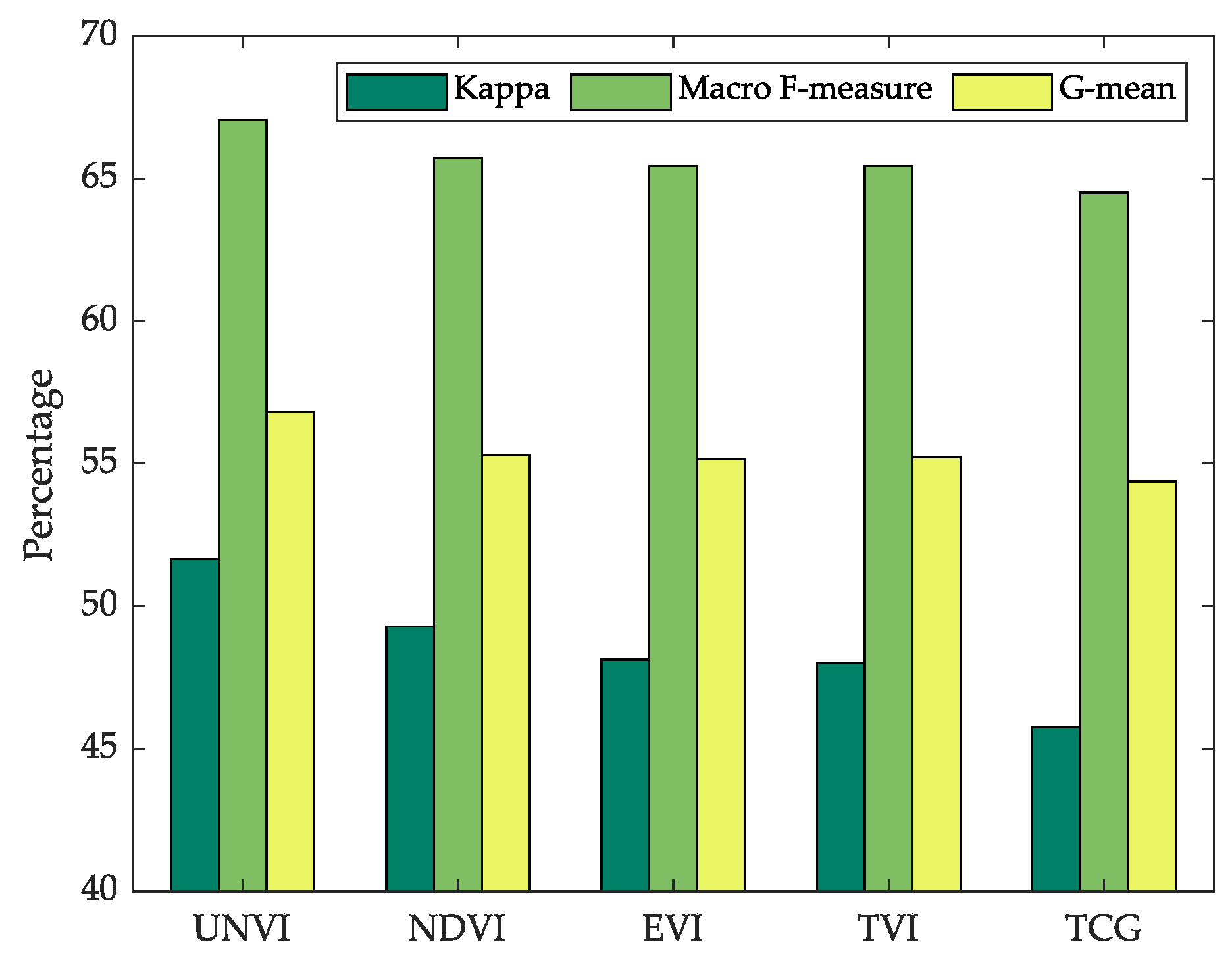
In the second experiment, RF classification was implemented to classify the five major vegetation classes in the study area. We chose RF instead of other classifiers, mainly based on the following considerations: (1) RF is the most commonly used algorithm in land cover classification using time series remote sensing data [
15,
16,
19,
53,
54,
74], so the results of RF classification are the most representative and convincing. (2) For classification problems, the results are usually susceptible to parameter tuning, so our comparative study is more inclined to use the classifier with fewer parameters, and RF has the reputation of this advantage, with two free parameters (
ntree and
mtry) relatively easy to tune [
52,
53]. For each VI, the features of VI time series and the further derived phenological parameters were used for classification. Although other features, such as time-series spectral bands, and DEM information, may be helpful to improve the classification performance, they may also have different importance of contributions to the classifier for different VIs, and thus could weaken or mess up the differences between these indices. So, for our evaluation and comparison purpose, only the features related to the VI time series were used for classification. The overall evaluation measures kappa coefficients, macro F-measures and G-means showed that UNVI slightly better classified the five vegetation classes. It should be underlined that for each VI, all the time series throughout the year and all the phenological parameters extracted from TIMESAT were used, which means that we tested the ultimate abilities of the VIs time series for classification. Thus, the differences between the accuracy measures of the classification results were not very substantial, which is consistent with the fact that JM distances of the five indices mostly approached 2.0 when all 23 time composites were used (see
Figure 6). On the other hand, Z-test results indicated that the classification results using UNVI time series were significantly better than using the other four VI time series.
Broadleaf, shrubs and grass were difficult to differentiate from each other, and they were often misclassified as each other. Because they have similar seasonal behaviors, and only differs in the canopy densities in the growing season. In particular, for the pair of broadleaf forests and shrubs, they are both made up of broadleaf deciduous trees in our study area, and differed only in the height of the trees (see the descriptions in
Table 1). So we got low JM distance and low classification accuracy when trying to discriminate broadleaf and shrubs. However, UNVI outperformed the other four VIs on discriminating these less distinguishable classes. This is mainly due to the fact that UNVI is more sensitive to LAI and thus better captures the subtle differences in canopy density between broadleaf and shrubs.
In this study, UNVI time-series performed outstandingly for the major vegetation discrimination in Chaoyang prefecture, mainly due to UNVI’s sensitivity to vegetation dynamics and high saturation point with respect to LAI. These advantages of UNVI also indicate that it has the potential to be used in vegetation dynamics related studies, such as estimating crop yield or vegetation productivity, where VI might be a key metric. Thus, we suggest the UNVI’s potential for characterizing and quantifying vegetation dynamics to be explored in future work. Additionally, as UNVI and NDVI outperform each other at different seasons for vegetation discrimination, the combination of UNVI and NDVI time series may be instructive, from the perspective of improving classification accuracy. So we also recommend that future work evaluates the effectiveness of combined VI time series for vegetation discrimination.
6. Conclusions
Time series vegetation index and the further derived phenological features have been widely used for land cover mapping. In previous studies, researchers used NDVI or EVI by default to generate temporal profiles. However, whether they are optimal VI for multi-temporal vegetation discrimination has not been evaluated. This study made an exploration on this issue, and investigated the vegetation discrimination ability of UNVI time series, in comparison with, NDVI, EVI, TVI, and TCG. We chose UNVI for evaluation mainly because of its full use of all spectral bands and its good performance in many application scenarios. Two comparative experiments, separability analysis and RF classification, were conducted. The results of our study indicate that:
For the overall separability of different types of vegetation, the UNVI is superior to EVI, TVI, and TCG, and almost equivalent to NDVI. During the dormant periods, NDVI performs better than UNVI due to the uncertain contribution of soils and yellow leaves to UNVI. However, during the peak of vegetation growing season, UNVI outperforms NDVI, EVI, TVI, and TCG, mainly because of its sensitivity to vegetation dynamics and high saturation point with respect to LAI.
UNVI times-series and its derived phenological parameters can better classify the five major vegetation classes than NDVI, EVI, TVI, and TCG, indicated by the comparisons of Kappa coefficients, Macro F-measures, and G-means.
For the most indistinguishable vegetation pair broadleaf and shrub, which differ only in the height of trees, UNVI achieves relatively larger JM distance and higher classification accuracy.
UNVI time-series therefore has considerable potential for regional land cover mapping. Thus, we could recommend using UNVI for future time series studies, such as vegetation classification, change detection and dynamic monitoring.


