Article

Monitoring Grass Phenology and Hydrological Dynamics of an Oak–Grass Savanna Ecosystem Using Sentinel-2 and Terrestrial Photography

by
Pedro J. Gómez-Giráldez
1,*,
María J. Pérez-Palazón
2,
María J. Polo
2 and
María P. González-Dugo
1
1
IFAPA. Institute of Agricultural and Fisheries Research and Training of Andalusia. Avd. Menéndez Pidal s/n, 14071 Córdoba, Spain
2
Fluvial Dynamics and Hydrology Research Group. Andalusian Institute for Earth System Research. University of Cordoba. Campus Rabanales, Edificio Leonardo Da Vinci, Área de Ingeniería Hidráulica, 14014 Córdoba, Spain
*
Author to whom correspondence should be addressed.
Remote Sens. 2020, 12(4), 600; https://doi.org/10.3390/rs12040600
Submission received: 26 December 2019 / Revised: 29 January 2020 / Accepted: 8 February 2020 / Published: 11 February 2020
(This article belongs to the Special Issue Remote Sensing of Savannas and Woodlands)

Abstract

:
Annual grasslands are an essential component of oak savanna ecosystems as the primary source of fodder for livestock and wildlife. Drought resistance adaptation has led them to complete their life cycle before serious soil and plant water deficits develop, resulting in a close link between grass phenology and soil water dynamics. In this work, these links were explored using a combination of terrestrial photography, satellite imagery and hydrological ground measurements. We obtained key phenological parameters of the grass cycle from terrestrial camera data using the Green Chromatic Coordinate (GCCc) index. These parameters were compared with those provided by time-series of vegetation indices (VI) obtained from Sentinel-2 (S2) satellites and time-series of abiotic variables, which defined the hydrology of the system. The results showed that the phenological parameters estimated by the S2 Normalized Difference Vegetation Index (NDVI) (r = 0.83, p < 0.001) and soil moisture (SM) (r = 0.75, p < 0.001) presented the best agreement with ground-derived observations compared to those provided by other vegetation indices and abiotic variables. The study of NDVI and SM dynamics, that was extended over four growing seasons (July 2015–May 2019), showed that the seasonality of both variables was highly synchronized, with the best agreements at the beginning and at the end of the dry seasons. However, stage changes were estimated first by SM, followed by NDVI, with a delay of between 3 and 10 days. These results support the use of a multi-approach method to monitor the phenology and the influence of the soil moisture dynamic under the study conditions.

Graphical Abstract

1. Introduction

Monitoring the phenology of Mediterranean ecosystems is key to adequately assessing the impacts of global warming on different time scales, identifying pre-critical states in the framework of early warning decision-making systems, and establishing adaptation planning and management in the medium- to long-term time horizons. The natural variability of the climatic–hydrological regime in these areas, usually with complex spatial patterns of the vegetation that is sometimes difficult to access, makes it necessary to exploit the available data from remote sensing sources.
The holm oak savanna ecosystem of the Iberian Peninsula (known as dehesa in Spain and montado in Portugal) is an ancient system emerging as the only productive and sustainable structure able to deal with the combination of low soil fertility and the high variability of the Mediterranean climate [1]. This landscape is formed by a low density of holm oak trees, an understory of grasslands and, occasionally, shrubs and crops of cereals and legumes. The result is a mixture of natural facto and management, making it difficult to differentiate the absolute determinants of its structure [2]. However, water availability is known to be important in the conformation of this mixture of grasses and woody plants which, as stated in [3], is the only stable state of equilibrium when a marked seasonality in water availability occurs. In this state, canopy density maximizes biomass, thus minimizing water stress [4]. Annual grasslands are an essential component of this system as the primary source of fodder for livestock, and is the main economic activity in these areas, but also contains a high richness of vascular plants supporting a wide diversity of habitats [5]. The escape mechanism—i.e., the ability for the plant to complete its life cycle before serious soil and plant water deficits develop [6]—is used by these grasses to cope with the long summer dry season and the recurrent water scarcity events of the Mediterranean climate. This results in a close link between grass phenology and soil water dynamics.
Plant phenological shifts have been observed as a result of changes in the climate [7,8,9,10]. Phenological research has advanced in developing climate–phenology models derived from ground observations [11,12] and also in improving the monitoring methods constructed from satellite information [13]. In recent years, the use of remote sensing in the study of phenology has increased thanks to a greater availability of global products, which allow one to extend these studies in space and time. In particular, the use of vegetation indices (VIs) has been generalized to determine changes in vegetation on different spatial scales, ranging from centimeters to tens of kilometers. Some examples are the use of the AVHRR (Advanced Very-High-Resolution radiometer) sensor for global studies [14,15,16]; broad scale analysis using MERIS (Medium Resolution Imaging Spectrometer) and MODIS (Moderate-Resolution Imaging Spectroradiometer) data for maize crops and forests [17,18]; studies on a detailed scale using Landsat or ASTER (Advanced Spaceborne Thermal Emission and Reflection Radiometer) for multiple crops monitoring [19,20]; and at a very high spatial resolution with UAVs (unmanned aerial vehicles) in vineyards [21]. The Sentinel-2 (S2) sensor, part of the European Union Copernicus Program, has provided the renewed possibility of addressing canopy phenological changes on a local scale with high spatial and temporal resolutions (10–20 m or 5 days), and an improved spectral resolution providing narrow bands in the red-edge region. Despite the short time series available (from July 2015 to present), S2 has been used for the monitoring of vegetation, addressing aspects such as phenology [22], complementing other sensor datasets such as MODIS [23] or Landsat [24], and monitoring biophysical variables through the proposal of new indices making use of the red-edge bands [25]. However, its potential for improving the accuracy of estimating the phenological transition stages has not been fully explored yet.
Remote sensing studies rely on field data of phenological parameters to explain their results. However, field monitoring requires frequent and time-consuming observations, especially over areas which are difficult to access. The use of digital terrestrial cameras offers a cost-effective solution, providing real-time and reliable information to track vegetation phenology. Previous studies have used cameras for phenological monitoring [26,27], and the creation of networks of these cameras for a more global phenological follow-up is being increasingly demanded [28]. In addition, these cameras can complement the information provided by other equipment, such as weather stations or eddy covariance systems, in a wide range of applications [29,30,31,32]. The combination of these ground observations with satellite images has also been explored [33,34,35], and the integration of highly detailed terrestrial photography with large-scale satellite images is a promising tool that could reduce the scale gap between phenological field and remote sensing studies.
The Mediterranean climate of this area presents a high vulnerability to global warming, with an increasing occurrence of extreme droughts and torrential rainfall. This region is projected to warm more and experience greater changes in the precipitation regime over the course of the century [36,37,38]. An improved knowledge of how climate and hydrology influence plant phenology is key to making appropriate decisions to cope with these threats [39]. In addition, changes in values of satellite VIs have proved to be able to reflect the heterogeneity of the hydrological behavior in this region [40]. In the same line, phenological variations, assessed by using satellite data, could be useful for evaluating the cumulative effect of the hydrological regime over large areas, in a capacity that would not be achievable with a field observation network.
In this work, images provided by a terrestrial camera were combined with meteorological information and satellite data to provide an insight into the dynamics of phenological processes and their links with the hydrological behavior of the grassland of an oak–grass savanna ecosystem. On this basis, the objectives of the present study were: (1) to explore the potential of the S2 satellites to monitor phenological changes over grasslands using a variety of vegetation indices derived from different band combinations, both broadband and narrowband indices, taking advantage in the latter case of the new possibilities offered by the red-edge bands of these satellites, (2) identify the links between hydrology and vegetation phenology derived from terrestrial photography, evaluating the response of grass vegetation and its life cycle to changes in the main abiotic variables controlling this system, and (3) study the relationship between satellite VIs and the hydrological state of the system regarding their ability to monitor grassland phenology.

2. Material and Methods

2.1. Study Site and Datasets

The study was conducted in a dehesa farm, called “Santa Clotilde” (Figure 1a), located in Southern Spain (Córdoba, 38° 12′ 37′’ N, 4° 17′ 24′’ W, 734 m.a.s.l.) [41]. It is part of an environmentally protected area (Sierra de Cardeña y Montoro Natural Park) with a landscape composed of sparse holm oak trees and natural grasses. The semiarid climate in this region is characterized by cold winters and long dry summers, with periodic severe droughts. Beef cattle and pigs are raised extensively on grasslands and acorns.
Field measurements were taken at a grass-dominated site (Figure 1b), in which the grasses were annual species of a medium size (with a maximum plant height between 0.5–1 m) and a variable coverage. The field has a great variety of species, chiefly grams such as Vulpia spp, Bromus spp or Aegilops spp, although legumes such as Trifolium spp, Ornithopus spp, Uncaria spp or Medicago spp are also found [42]. The soil at the site is dominated by Eutric Cambisols, with a loamy sand texture in the grass root zone (0–30 cm). The soil moisture content, modeled at field capacity (FC) and wilting point (WP) [43], was equal to 0.18 and 0.08 m3/m3, respectively.
The site’s instrumentation included a digital camera, micrometeorological equipment and soil moisture probes. Terrestrial photography was acquired using a CC5MPX Digital Camera (Campbell Sci. Inc) installed at a height of 1.65 m above the ground surface. This is a programmable camera of 5 megapixels which has been specially prepared to be placed outdoors (at a thermal amplitude –40 to 60 °C). Its field of view (FOV) is 790 square meters (Figure 1b), and images were obtained from the installation every hour over the daylight period, generally from 8 a.m. to 6 p.m., from the beginning of December 2017 to the end of May 2019.
According to data availability, two study periods were defined: a first period, herein called A, from December 2017 to May 2019, with available terrestrial images on a daily basis measuring field grassland greenness, and an extended period of analysis (study period B), from July 2015 to May 2019, which covered the whole period with Sentinel-2 availability (since first acquisition time).
The set of abiotic variables measured at the site during the whole study period (Figure 1b) included the following:
  • Air temperature, recorded using an HMP45A probe (Vaisala OyJ); daily minimum (Tmin), maximum (Tmax) and mean temperature (Tmed) values were computed from half-hourly records.
  • Incoming and outgoing solar radiation (Rad), measured with a four-way radiometer NR-01 (Campbell Sci. Inc); daily cumulative radiation fluxes were computed from half-hourly records.
  • Vapor pressure deficit (VPD) was derived from atmospheric pressure and relative humidity (HMP45A probe (Vaisala OyJ); daily values were computed from half-hourly records.
  • Precipitation (R) was measured with a weighing-type recording rain-gauge ARG100 (Campbell Sci. Inc); daily values were computed from the aggregation of 30 min cumulative values.
  • Volumetric soil moisture (SM) was measured at two depths (10 and 30 cm) with an ENVIROSCAN (Campbell Sci. Inc) probe at 10 min intervals. Daily values were computed from these data and averaged between both depths.
Figure 2 shows the general meteorological characterization of the study period with monthly values of R and Tmed and the monthly average of the province of Córdoba with historical data from 1971–2000 [44]. A very irregular annual distribution of rainfall was observed, as expected, as well as a great thermal amplitude on different time scales. Compared with the historical values, the four hydrological years of the study period could be considered within the average regime in terms of mean temperature, with values in summer close to 30 °C that may drop below 10 °C in winter, and mean annual temperature of 16 °C. In terms of total precipitation, the historical annual value in the area was about 650 mm: 2015/2016 and 2016/2017 were normal periods (close to 700 mm) but with different temporal distributions; 2017/2018 was an anomalous year in the seasonal distribution of precipitation in that it was drier than average until the month of March, in which 356 mm of the final 820 mm of annual precipitation was concentrated; and 2018/2019 was the driest period (500 mm).
The satellite image dataset consisted of 242 granules of Sentinel-2 images. It included all available images with less than 15% of cloud coverage from July 2015 to May 2019. From March 2017 to May 2019, the atmospherically corrected product Level 2A available from ESA (European Space Agency) was used. From July 2015 to March 2017, the images were atmospherically corrected using the module Sen2cor included in SNAP (ESA Sentinel Application Platform v2.3.0). Seven bands were processed to compute the different vegetation indices used in this study (the central wavelength and the bandwidth are indicated in parentheses): B2 = blue (492 nm; 66 nm), B3 = green (559 nm; 36 nm)), B4 = red (665 nm; 31 nm), B5 = red edge 1 (704 nm; 15 nm), B6 = red edge 2 (740 nm; 15 nm), B7 = red edge 3 (783 nm; 20 nm) and B8 = near infrared (NIR) (833 nm; 106 nm).

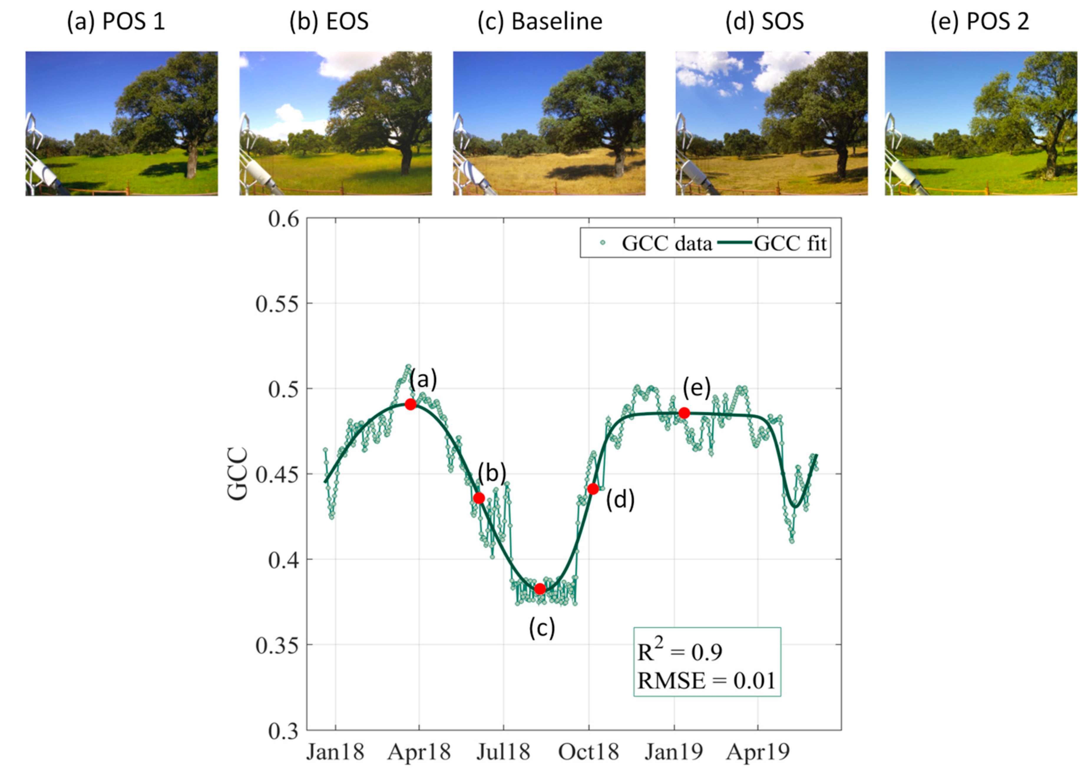
2.2. Phenological Parameters From Terrestrial Photography

The greenness of the grass, observed by terrestrial photography, was used as a field indicator of grass phenology and used to evaluate the phenological parameters retrieved from the satellite images. A quantitative value of this greenness was computed using the Green Chromatic Coordinate (GCC) (Equation (1)) [45]. The GCC index is not a direct measurement of chlorophyll content, and previous research [35,46,47] has addressed its sensibility to changing levels of green pigmentation in vegetation and how canopy phenology can be monitored and quantified without the need for a human observer. This index is a non-linear transformation of the digital levels of the green color of the picture, and it is known to minimize the effects of different lighting between images taken on different days. Their characterization of greenness has proved to be better than those of other camera indices [48]:
G C C = G R + G + B
where
  • GCC: Green Chromatic Coordinate index;
  • R: digital level in red;
  • G: digital level in green;
  • B: digital level in blue.
This index was calculated as the average value of the pixels of a homogeneous grass region of interest (ROI) (Figure 1c). Daily index values were computed for period A (December 2017 to May 2019) using the 90th percentile, in which all the GCC values were used in a 3-day moving window, assigning the average value to the central day. This methodology is assumed to reduce the error in the estimates by more than 30% [49].
To calculate the phenological parameters from GCC values, the 50% amplitude method [50] was used. In this method, the temporal evolution of a variable is considered as a function, and the state changes are supposed to be within 50% of the amplitude of this function. The amplitude was fixed for each annual growing cycle as the difference of the minimum GCC (baseline value) and the maximum value (peak value). The parameters calculated were as follows:
Start of season (SOS): time when 50% of the amplitude is reached.
Peak of season (POS): time when the data reach the maximum value of the cycle.
End of season (EOS): time when 50% of the amplitude is reached to the right of the peak value.
To homogenize the extraction of values, the data were fitted using a double logistic function (Equation (2)), which is commonly employed to process remotely sensed data for phenology monitoring [51,52,53]. This function has proved to be useful for reducing the noise in a satellite time-series and enforcing a general seasonal shape on noisy data [54].
v ( t ) = v m i n + v m a x ( 1 1 + e x 1 y 1 t 1 1 + e x 2 y 2 t ) v ( t )   =   v
where
  • v(t): value of the function at time t;
  • vmin: minimum value of the amplitude;
  • vmax: maximum value of the amplitude;
  • x and y: parameters that control the shape of the curve. x1 and x2 control the left and right inflexion points, respectively, and y1 and y2 represent the rate of change at time t.
The TIMESAT program [51,54,55] was used to fit the double logistic function to the time series and extract the phenological parameters.

2.3. Selection of Satellite Vegetation Indices

The time series of various vegetation indices, derived from Sentinel-2 images, were studied to evaluate their ability to capture the phenology of the vegetation observed in the field using terrestrial photography. An initial set of VIs, listed in Table 1, were calculated and spatially averaged in the FOV given in Figure 1b. The first group of broad-band indices included the Normalized Difference Vegetation Index (NDVI) [56], and a version of this which changed the red reflectance for the green one—the Green Normalized Difference Vegetation Index (GNDVI) [57]; the Soil Adjusted Vegetation Index (SAVI) [58]; the Enhanced Vegetation Index (EVI) [59] and a simplified version, EVI2 [60]. The new possibilities of Sentinel-2 red edge bands made a second group of narrowband indices possible, including an adaptation of the Meris Terrestrial Chlorophyll Index (MTCI) [61] and two indices developed specifically for Sentinel-2 data: the Inverted Red Edge Chlorophyll Index (IRECI) and Sentinel-2 Red Edge Position (S2REP) [25]. Finally, GCC was computed using Sentinel-2 bands and was named as GCCs to distinguish it from the GCC from the camera, herein called GCCc. All VIs were calculated for the whole study period and spatially averaged at the camera FOV.
Once the indices values were obtained for Sentinel-2 acquisition days, a daily time series for period A was computed using a linear interpolation between every two consecutive images. To minimize the effect of possible spikes due to clouds or poor atmospheric conditions, daily index values were smoothed using the Savitzky–Golay filter [62]. This method replaces each data value by a linear combination of nearby values in a moving window, helping to reduce the noise and producing a higher quality VI time series [63]. These satellite-derived time series were compared with GCCc values for the same period; the statistical analysis was able to identify those of satellite VI better on reproducing the digital camera observations. In order to compare the performance of the different indices, their values were normalized.
Similar to GCCc, satellite VI time-series were fitted to a double logistic function, and the 50% amplitude method was applied to estimate the phenological parameters, comparing their results with those obtained from GCCc data.

2.4. Selection of Abiotic Variables

The daily evolutions of different weather variables together with the water content of the root-depth soil layer were studied to locally evaluate their links with vegetation phenology and to obtain information on the main factors influencing their behavior.
The set of abiotic variables initially selected were those commonly identified in phenological studies (Tmax, Tmed and R), the meteorological variables often used in crop growth models (Tmin, Rad and VPD), and the water content in the root depth of the soil layer of the grasses (SM). Daily data were obtained from half-hourly values of the weather station for the period December 2017 to May 2019, as described in Section 2.1.
The relationship between these variables and the daily series of GCCc were analyzed throughout period A. The principal explanatory variable was also employed to determine phenological parameters by fitting its values to a double logistic function, as described previously, and applying the 50% amplitude method.

2.5. Satellite VI and Abiotic Variable Relationship

The dynamic of the selected satellite VI and the most significant abiotic variable were compared during period B (July 2015 to May 2019). For this purpose, data from both of them for this period were fitted to a double logistic function, and the phenological parameters were extracted in the same way as period A.

2.6. Statistical Analysis

To evaluate the relationships between the GCCc, satellite VIs, and the abiotic variables, a Pearson correlation matrix and principal component analysis (PCA) were carried out to detect the group of variables that similarly governed the behavior of the system [64]. This method generates a new set of variables, called principal components (PCs), which are linear combinations of the original ones. The variables are related by coefficients that range between −1 and 1. The closer to 1 or −1 they are in a certain PC, the higher the direct or inverse influence they exert, respectively, on the PC. All the PCs are orthogonal to each other, so there is no redundant information. Once the PCs are obtained, all the variables of the system are grouped by processes. Since the original variables have different dimensions, standardization was applied prior to the PCA by dividing each one by its standard deviation. This process was applied firstly to GCCc with satellite VIs in order to select the representative ones, and, secondly, to GCCc with the abiotic variables.
The TIMESAT program was used to fit a double logistic function to all the variables’ time series and extract the phenological parameters. Finally, the coefficient of determination (R2) and the root mean square error (RMSE) were used to evaluate the results.
All these calculations and statistical treatments were conducted by programming in MATLAB (The Mathworks Inc., MA). The algorithms used were corcoeff for Pearson correlation matrices, pca for PCA and the Curve fitting tool for R2 and RMSE.
To assess the relationship between the phenological parameters estimated using the indices, the differences in days i.e., the biases with respect to the values obtained by the GCCc were computed, and the percentage of those biases was calculated with respect to the total length of the phenological cycle, with an estimated value of 210 days (seven months) as an average [1]. In the case of the joint assessment of satellite VI and the abiotic variable, the bias in days was also calculated.

3. Results

3.1. Deriving Phenological Parameters From Terrestrial Photography

Figure 3 shows the evolution of the GCCc values throughout period A consisting of one and a half growing seasons and the function fitted to those data. The days when the baseline, SOS, EOS and the two POS for the period were reached have been identified, and the pictures (Figure 3a–e) illustrate the state of the grass at each phenological stage.
The lack of a first cycle starting point and the ending of the second one prevented the analysis of a complete single cycle. The start of the period coincided with the installation of the camera; the premature end of the second cycle was artificial and due to common farm management practices, i.e., plowing and preparing the soil for a future cereal crop. Thus, the parameters to be studied were the EOS of the first cycle, the SOS of the second and the peaks of both cycles. The baseline value used was the summer minimum of 2018.
The fitted function presented a high correlation of R2 = 0.9 and a very low error of RMSE = 0.01. It can be seen that the dates of the phenological parameters given by the 50% amplitude method correctly matched the observations derived from the visual inspection of the digital camera photographs. Both POSs showed a green full cover; in the baseline, the grass was totally dry, and EOS and SOS showed the beginning of senescence and the grass becoming green, respectively.

3.2. Terrestrial Camera vs. Satellite-derived Indices

3.2.1. Satellite and Ground-based Indices Comparison

The behavior of the different satellite indices and GCCs in the study area was analyzed using the histograms of the values obtained during a complete growing cycle (year 2018). Figure 4 presents the distribution of the normalized VI values throughout this year. It can be observed that some variability was derived from the different algorithms and band combinations. All indices presented a first peak corresponding to low/very low values. This peak was more pronounced for EVI2, SAVI, IRECI and GCCs. Most indices also presented a second peak corresponding to intermediate/high index values. NDVI, EVI, GNDVI showed a more balanced distribution between both peaks than the previous group. However, MTCI and S2REP shapes do not completely follow this general pattern.
Table 2 shows the Pearson correlation coefficients of daily time series of GCCc with the daily time series of a selection of satellite-derived VIs.
The correlation of all satellite indices with GCCc was significant (p < 0.001) and had a high correlation value (r > 0.7), except for MTCI and S2REP (r = 0.52 and –0.44, respectively).
The results for PCA are shown in Figure 5. Most of the variance (79%) was explained by the PC 1, in which two groups of indices could be distinguished: a first group of higher coefficients (equal to or greater than 0.3) included GCCc and GCCs with the rest of the satellite indices except the MTCI and S2REP, which would together form a second group with lower or negative coefficients. In turn, these two indices presented higher values (> 0.5) in PC 2, which explained 11% of the total variance.

3.2.2. Satellite-derived Phenology

Based on the results of the previous section, VIs with a correlation higher than 0.7 and placed in the same group of data in PCA were selected for the subsequent analysis. Thus, seven satellite VIs were selected for the phenological analysis: EVI, EVI2, GCCs, GNDVI, IRECI, NDVI, and SAVI.
The smoothed daily data from the fitted functions are shown in Figure 6 together with the phenological parameters obtained from those VIs.
All fitted functions showed very high correlation values (R2 > 0.95) and low RMSEs (<0.03).
It can be observed (Figure 6) that the EOS was the parameter which was most similarly estimated by all indices and had the lowest bias with respect to the GCCc. The estimation of both POSs presented a higher dispersion. For this reason, POS 1 and POS 2 derived from the original raw data have been also included in Table 3 in addition to the values derived from the adjusted functions. These data are not presented for the EOS and SOS parameters due to the observed existence of erratic spikes that may cause erroneous estimations of green-up or real senescence shifts. Table 3 summarizes the biases of the phenological dates of the satellite VI with respect to GCCc (Figure 6b).
The estimation of the green up (SOS) was delayed by all satellite VIs, with GCCs, GNDVI and NDVI presenting the lowest errors of around ten days (less than 10% of the cycle). The agreement was higher for the end of the season, with errors below 10% in all cases and biases of only one day using NDVI and SAVI. For both peaks of the season, there was a general delay in the estimations, with lower errors in POS 1 than in POS 2 in most cases. EVI and NDVI produced the best results for POS1, and GCCs and NDVI for POS 2. However, in the case of POS, the dates obtained using the original raw data generally improved the estimates. It could be of interest to evaluate the impact of specific weather events. In general, NDVI obtained the most consistent results and lowest errors; considering this, NDVI was selected for further analysis in this work.

3.3. Analysis of Abiotic Variables and Greenness Dynamics

The results of the Pearson correlation matrix between the daily time series of GCCc and the daily time series of selected abiotic variables for period A are shown in Table 4. All correlations were significant (p<0.001), and soil moisture (SM) presented the highest correlation (r = 0.75). Some variables, including VPD, Rad, Tmin, Tmed, and Tmax, were inversely correlated with greenness. Rainfall, although positively correlated, presented the lowest coefficient of all analyzed variables. In the PCA results (Figure 7), the first PC explained 60% of the total variance, showing high coefficients (greater than 0.3) for most variables. Similar to the correlation matrix results, a first group with negative coefficients included GCCc and variables favoring an increase of soil water content (SM and R); a second group with positive coefficients was formed by variables with high values during the summer when the grass canopy was dry.

Grassland Phenology and Soil Moisture Relationship

Considering the previous results, SM has been selected to evaluate its capability to predict the phenology of the grass canopy of oak–grass savanna ecosystems. Figure 8a shows the distribution of SM data and the fitted function. This function presented a correlation of R2 = 0.9 and an error of RMSE = 0.02, indicating a good agreement, although to a lesser extent than those obtained for GCCc and satellite VIs.
The phenological parameters predicted by this function were compared to those derived from GCCc (Figure 8b). The SOS and EOS were quite similar to the timings estimated by GCCc, with a slight advance in both dates according to SM estimations. The 50% amplitude method resulted in similar values of SM, around 0.14 m3 /m3 on average, marking the beginning and the end of the growing season.

3.4. Relationships Between Soil Moisture and NDVI

The relationship between NDVI and SM—i.e., the variables that best suited the phenological monitoring of the grassland according to the previous results—were analyzed during period B (July 2015 to May 2019) comprising a total of four growing seasons.
Figure 9 shows the data for SM, the smoothed data for NDVI, the functions fitted to both series, and the phenological parameters extracted from them. The marked and mostly synchronized seasonality of both variables can be observed. The highest differences were found during the second year, corresponding to the growing season 2016/2017, with differences of 9 days (4.3%) for SOS, 28 days (13.3%) for POS and 16 days (7.6%) for EOS. Both fitted functions showed a high correlation (R2 = 0.9 for SM and R2 = 0.93 for NDVI) and low errors (RMSE = 0.02 for SM and RMSE = 0.04 for NDVI). Compared to GCCc, NDVI showed a later response to water availability, resulting in lower differences in monitoring the phenology.

4. Discussion

4.1. Capability of the Terrestrial Photography to Provide Phenological Parameters

The two hydrological years of study period A are an example of Mediterranean climate variability (Figure 2), and therefore of phenology variability. In 2017/2018, most of the precipitation was concentrated in a short period of time at the beginning of March, and POS 1 occurred shortly after those intense events. On the other hand, 2018/2019 was a drier year, but with a more regular rainfall distribution in the fall and spring. A lower GCCc maximum value was reached, but the growing season was longer, producing a plateau shape in which an intermediate value was identified as POS 2.
GCCc values ranged between 0.35 and 0.5, reaching their maximum values between November and April, eventually presenting drops of varying duration and intensity due to the particular weather conditions of the year. This temporal trend of the GCCc time series was similar to the one observed by other studies in Mediterranean grasslands [65,66]. The reasonable behavior of the CGGc of canopy status in the field according to the weather conditions, the previous studies and the visual observations provided by the terrestrial photography supported the use of GCCc time series as a reference to evaluate the performance of satellite vegetation indices.

4.2. Comparison of Ground and Satellite-based Indices

The first peak with a low value observed in Figure 4 corresponds to a predominance of dry grass/bare soil coverage during the dry season. Indices particularly sensitive to soil contribution, such as EVI, EVI2 and SAVI [58], present a higher concentration around these low values. The second peak may correspond to the central time of the spring, when the greening is widespread, while intermediate values reflect periods of green-up and senescence. The narrow band indices (IRECI, MTCI and S2REP) showed a wider distribution in values, probably due to the greater sensitivity to the changes that the red edge presented. It is worth mentioning that NDVI and GNDVI presented a sharpened ending at high values compared to other indices, with an accumulation of intermediate–high values that did not reach its maximum. This might indicate a certain degree of saturation of both indices under high grass cover conditions. This issue, described in previous studies for forest or high biomass crops [67,68], appears to occur here also to some extent. It is also worth noting the difference in the distribution of GCCs and GCCc; with the same formulation, the satellite version presented lower values than those calculated using the field camera. This result could have been due to the differing geometry of the image acquisition.
The low correlation for MTCI shown in Table 2 could be explained by the rapid response of this index to chlorophyll variations [61]. This causes the time series to follow a different trend than the rest of the indices, which is more connected to green foliage density [69] with smoother transitions. MTCI has presented good results in more homogeneous canopies, such as subalpine grasslands [33] or in deciduous trees in Central Europe [70]. In this case, the high diversity of species, typical of Mediterranean grasslands, might explain the high variability observed in these values. The case of S2REP is similar since it was also designed to measure chlorophyll variation using three bands located in the red-edge region, and allegedly provides a better characterization of the red-edge slope than MTCI [25]. IRECI also uses three bands in the red edge, although the high correlation presented with GCCc might be explained by a different formulation. In this case, the index was designed to focus on the chlorophyll content of the canopy instead of the leaf scale addressed by S2REP [25]. The influence of the vegetation ground coverage and foliage density was higher and more similar to the other broad-band indices.
The results for PCA in Figure 5 showed that most of the variance (79%) was explained by the PC 1, in which two groups could be distinguished; a first group of higher coefficients (equal to or greater than 0.3) included GCCc and the rest of the satellite indices except the MTCI and S2REP, which would form a second group with lower or negative coefficients. In turn, these two indices had high values (>0.5) in PC 2, which explained 11% of the total variance. This grouping confirmed the results obtained by the Pearson correlation and suggested that these two red-edge indices might be related to a different process than the rest. In that case, MTCI and S2REP would be more useful for estimating leaf chlorophyll content [61,71], while the rest were more influenced by canopy foliage. Regarding the pixel size, it does not seem to have had an influence on previous results or to determine the selection of the index for the conditions of this study. IRECI, at 20 m in size (like MTCI and S2REP), was included in the subsequent phenological analysis.
The estimation of the green up (SOS) was delayed by all satellite VIs, but GCCs, GNDVI and NDVI presented low errors of around ten days (less than 10% of the cycle). The agreement was higher for EOS, with errors below 10% in all cases and biases of only one day using NDVI and SAVI. However, in the case of POS, the dates obtained using the original raw data generally improved the estimates—something of interest to evaluate the impact of specific weather events—nevertheless, in the case of analyzing long time series, fitted functions provide a useful homogenization procedure, generally leading to a more consistent analysis.
The disagreement in terms of POS estimations between satellite-borne and ground-borne sensors can be explained by the different acquisition angle of both systems. The field camera captures flowering and the presence of non-photosynthetic elements such as stems [46], which might reduce greenness and anticipate peak time. Despite this factor, NDVI exhibited a very similar behavior to GCCc, with lower differences in days than those of previous studies in grasslands [66,72]. A possible reason for the comparatively lower errors could be the higher spatial resolution employed in this case (10 m for Sentinel-2 versus 250 or 500 m for MODIS, as previously used). This factor may become a major issue in mixed grass/tree systems [34]. GNDVI also provided good general results for EOS and SOS, although POS, especially for the first year, was somewhat delayed. GCCs, with the same formulation as GCCc, presented higher errors than NDVI when applied to satellite bands. EVI, EVI2, IRECI and SAVI displayed the highest difference of days in this study, despite EVI2 and NDVI having performed similarly in other types of grasslands [47] and with even better EVI2 results for maize yield [73] and EVI for deciduous tree coverages ([74,75]). In general, NDVI obtained the most consistent results and the lowest errors (less than 10% in all cases). These good results support the use of this multi-scale approach to complement phenology studies in grasslands. Even though the availability of terrestrial camera observations is not widespread, the increasing number of these stations is a promising framework to encourage this combined strategy.

4.3. Analysis of the Dynamics of Abiotic Variables, Greenness and Phenology

The results shown in Table 4 are consistent with the water-limited condition of this ecosystem, where the dynamics of plant development and soil moisture are intimately related. This explains the high correlation of SM with GCCc, and the positive values found for SM and rainfall, with both variables favoring an increase in soil water content. The low correlation coefficient of the rainfall was also reasonable considering the daily time scale and the bulk analysis performed over a period with high rainfall variability. Rainfall has been previously related to the timing of leaf flush in dry forest [76], suggesting that an event-based analysis at specific times of the year might produce different results. High values of solar radiation, air temperature and VPD—characteristics of the dry season—are linked to an increase in atmospheric water demand, thus accelerating the water stress process in the vegetation and explaining the inverse relationships with grass greenness. This general description of the ecosystem behavior is also supported by PCA results (Figure 7). The first PC explained 60% of the total variance, showing high coefficients (greater than 0.3) for most variables. Similar to the correlation matrix results, a first group with negative coefficients included GCCc and variables favoring an increase in soil water content (SM and R); a second group with positive coefficients was formed by variables with high values during the summer when the grass canopy was dry. These variables might negatively influence the plant water status in water scarce conditions. No significant differences in both analyses were obtained when the different growing season stages were analyzed separately.
Analyzing the behavior of SM shown in Figure 8, the value of SM selected by the 50% method for the EOS seems slightly high, as it coincides with a fraction of around 60% of the total available soil water. This depletion fraction is close to the threshold used for crops [77] below which the soil water can no longer be transported quickly enough towards the roots to meet the transpiration demand, and the plant starts to experience stress. However, in this application, this threshold is supposed to indicate the complete senescence of the plant rather than the beginning of plant water stress, which might indicate that both processes—the soil drying and the response of the vegetation—happened very quickly.
The use of SM to compute the POS in this environment makes less sense than for SOS and EOS, and the biases found with respect to GCCc estimations confirm this point. First of all, the data reflected a significant difference between the two POSs reached in the field-calibrating period as a consequence of the natural climatic variability of this region. POS 1 estimation with SM was closer to GCCc estimation, occurring with a bias of 9 days (4.3%). For POS 2, the bias was of –23 days (11%), presenting a difficult identification of the peak due to a flatter distribution of SM over the mid-growing season. Looking at the distribution of GCCc (Figure 3) and SM (Figure 8a), the shape of the first cycle was sharper because high SM values were concentrated in a short period, producing a fast response in GCCc values, with the POS reached before the SM peak, once the plant had no limitation to accessing soil water. In the second cycle, the distribution of SM followed a distribution with two similar low peaks (November 2018 and February 2019) with a slightly drier period around January. This reduction in SM was reflected by both GCCc (Figure 3) and some satellite VIs such as NDVI or GCCs (Figure 6), confirming the close link between SM and greenness and also the fast response of the vegetation to relatively small reductions in SM. This change in SM was small and it was not reproduced by the different fitted functions however, nevertheless, it caused a notable bias in the peak identification. Using the unfitted data for the POS, the results were similar; in POS 1, there was an advance of 9 days (4.3%), and in POS 2, this was 31 (14.7%).

4.4. Relationship Between SM and NDVI

The synchronized seasonality of both variables observed in Figure 9 has already been pointed out for other vegetation types under arid or semi-arid conditions in [78], in which the authors reported an increasing synchronization following a gradient of dry season length in a region. It is worth noting here the similar shapes of both variables following the beginning and the end of the dry periods, supporting the higher control of soil moisture on vegetation development during those periods. In general, an average delay between 3 and 10 days can be noted in the estimation of most phenological parameters with NDVI with respect to SM. The highest differences were found in the second year, corresponding to the growing season 2016/2017, with differences of 9 days (4.3%) for SOS, 28 days (13.3%) for POS and 16 days (7.6%) for EOS. During that year, the grassland was plowed and sown in the middle of February, following a management practice conducted every nine years or so that is currently disappearing in the area. Therefore, these two grass-growing cycles were artificially shaped and were not adequately reproduced by the fitting function. The poor adjustment of the function affects the phenological estimations, increasing their errors. Apart from this specific case, both fitted functions showed a high correlation (R2 = 0.9 for SM and R2 = 0.93 for NDVI) and low errors (RMSE = 0.02 for SM and RMSE = 0.04 for NDVI). Compared to GCCc, NDVI showed a later response to water availability, resulting in lower differences in monitoring the phenology. However, this difference could simply be due to the lower temporal resolution of satellite data, with a minimum of 5 days, compared to the daily availability of the terrestrial photography.

5. Conclusions

The phenology of a semi-arid grassland was monitored using terrestrial photography, satellite images, and abiotic ground measurements. The similarities and discrepancies observed using these datasets supported the capability of satellite vegetation indices to track important phenological parameters of this canopy and highlight the close relationship between these phenological parameters and the soil moisture dynamic under the study conditions.
The methodology to process the ground and satellite time series and extract the phenological information, implemented in TIMESAT, successfully fitted the data, with high correlation coefficients and low errors (R2> 0.9 and RMSE < 0.03 in all cases at the two scales), and identified key seasonal changes of the natural grasslands. On the ground, daily time series of the GCCc, computed using digital photography, estimated grassland phenological parameters in accordance with visual inspection and with the observed climatic conditions of the experimental study period. On the S2 satellite platform, NDVI was the index that better reproduced ground GCCc behavior, with the highest correlation (r = 0.83) and less than 10 days of difference for all the phenological parameters studied (representing less than 5% error within a grass cycle). None of the VIs using bands in the red-edge region improved the NDVI results. Two of them, MTCI and S2REP, followed a different trend than the rest of the explored indices. Both indices presented a high temporal variability, which could be explained by chlorophyll content variations caused by the diversity of species of this grassland, different to the more homogeneous canopies of previous studies [33,70]. The rest of the indices were more related to foliage density [69] and presented smoother changes in this canopy.
The abiotic variable that best represented the behavior of GCCc was SM (r = 0.75). The estimation of SOS and EOS phenological parameters using SM time series presented a good agreement with GCCc, with SM reaching threshold values a few days before greenness ones, as measured by GCCc. The values of SM found at the beginning and the end of the growing seasons, when changes between green and senescent stages occurred, were high according to the modeled soil water holding capacity. This might indicate that these modeled values were not accurate enough to assess the quick response of this canopy to the soil drying process. On the other hand, SM was not a good indicator of the POS, presenting significant biases with respect to GCCc estimations.
Finally, the behavior of NDVI and SM during the four growing seasons points out the synchronized seasonality shown in this system by the vegetation greenness, measured here by the NDVI and the SM. Higher agreement was found at the beginning and the end of the dry season, with stage changes estimated first by SM followed by NDVI with a delay of between 3 to 10 days. Taking into account these results, it is possible to monitor the water state of the soil from the phenological parameters obtained with NDVI of S2 and also to determine the phenological state of the cover from the SM with errors below ten days for this type of coverage.

Author Contributions

Conceptualization, P.J.G.-G. and M.P.G.-D.; methodology, P.J.G.-G., M.P.G.-D., M.J.P.-P. and M.J.P.; software, P.J.G.-G. and M.J.P.-P.; data curation, P.J.G.-G.; writing, review, and editing, P.J.G.-G., M.P.G.-D., M.J.P.-P. and M.J.P.; graphical deployment, P.J.G.-G. and M.J.P.-P.; supervision, M.P.G.-D. and M.J.P. All authors have read and agreed to the published version of the manuscript.

Funding

This work was supported by the SensDehesa (PP.PEI.IDF201601.16) project, co-funded at 80% by the European Regional Development Fund (ERDF), as part of the Andalusian operational program 2014–2020; additional support was provided by the project “Control and early warning of critical ecohydrological states in areas of Dehesa and high mountains through terrestrial photography”, funded by the Biodiversity Foundation, Spanish Ministry of Agriculture, Fisheries, Food, and Environment.

Acknowledgments

The authors are grateful to the owner of the Santa Clotilde farm for providing access to the site.

Conflicts of Interest

The authors declare no conflicts of interest. The funders had no role in the design of the study; in the collection, analyses, or interpretation of data; in the writing of the manuscript, or in the decision to publish the results.

References

  1. Olea, L.; Miguel-ayanz, A.S. The Spanish dehesa, a traditional Mediterranean silvopastoral system. In Proceedings of the 21st General Meeting of the European Grassland Federation, Badajoz, Spain, 3–6 April 2006; pp. 1–15. [Google Scholar]
  2. Scholes, R.J.; Archer, S.R. Tree-Grass Interactions in Savannas. Annu. Rev. Ecol. Syst. 1997, 28, 517–544. [Google Scholar] [CrossRef]
  3. Eagleson, P.S.; Segarra, R.I. Water-Limited Equilibrium of Savanna Vegetation Systems. Water Resour. Res. 1985, 21, 1483–1493. [Google Scholar] [CrossRef] [Green Version]
  4. Eagleson, P.S.; Tellers, T.E. Ecological optimality in water-limited natural soil-vegetation systems: 2. Tests and applications. Water Resour. Res. 1982, 18, 341–354. [Google Scholar] [CrossRef] [Green Version]
  5. Moreno, G.; Gonzalez-Bornay, G.; Pulido, F.; Lopez-Diaz, M.L.; Bertomeu, M.; Juárez, E.; Diaz, M. Exploring the causes of high biodiversity of Iberian dehesas: The importance of wood pastures and marginal habitats. Agrofor. Syst. 2016, 90, 87–105. [Google Scholar] [CrossRef]
  6. Turner, N.C. Drought resistance and adaptation to water deficits in crop plants. Stress Physiol. Crop Plants 1979, 343–372. Available online: https://ci.nii.ac.jp/naid/10006285376/en/ (accessed on 25 December 2019).
  7. Parmesan, C.; Yohe, G. A globally coherent fingerprint of climate change impacts across natural systems. Nature 2003, 37–42. [Google Scholar] [CrossRef]
  8. IPCC 2001. Climate change 2001: Impacts, adaptation, and vulnerability. Contribution of Working Group II to the third assessment report of the Intergovernmental Panel on Climate Change (IPCC). In Choice Reviews Online (Vol. 39); McCarthy, J.J., Canziani, O.F., Leary, N.A., Dokken, D.J., White, K.S., Eds.; Cambridge University Press: Cambridge, UK, 2001. [Google Scholar] [CrossRef]
  9. Parmesan, C. Influences of species, latitudes and methodologies on estimates of phenological response to global warming. Glob. Chang. Biol. 2007, 13, 1860–1872. [Google Scholar] [CrossRef]
  10. Cleland, E.E.; Chuine, I.; Menzel, A.; Mooney, H.A.; Schwartz, M.D. Shifting plant phenology in response to global change. Trends Ecol. Evol. 2007, 22, 357–365. [Google Scholar] [CrossRef]
  11. Menzel, A. Phenology: Its importance to the global change community—An editorial comment. Clim. Chang. 2002, 54, 379–385. [Google Scholar] [CrossRef]
  12. Rafferty, N.E.; CaraDonna, P.J.; Burkle, L.A.; Iller, A.M.; Bronstein, J.L. Phenological overlap of interacting species in a changing climate: An assessment of available approaches. Ecol. Evol. 2013, 3. [Google Scholar] [CrossRef]
  13. Fisher, J.I.; Richardson, A.D.; Mustard, J.F. Phenology model from surface meteorology does not capture satellite-based greenup estimations. Glob. Chang. Biol. 2007, 13, 707–721. [Google Scholar] [CrossRef]
  14. Justice, C.O.; Townshend, J.R.G.; Holben, A.N.; Tucker, C.J. Analysis of the phenology of global vegetation using meteorological satellite data. Int. J. Remote Sens. 1985, 6, 1271–1318. [Google Scholar] [CrossRef]
  15. Reed, B.C.; Brown, J.F.; VanderZee, D.; Loveland, T.R.; Merchant, J.W.; Ohlen, D.O. Measuring phenological variability from satellite imagery. J. Veg. Sci. 1994, 5, 703–714. [Google Scholar] [CrossRef]
  16. Jin, Z.; Zhuang, Q.; He, J.S.; Luo, T.; Shi, Y. Phenology shift from 1989 to 2008 on the Tibetan Plateau: An analysis with a process-based soil physical model and remote sensing data. Clim. Chang. 2013, 119, 435–449. [Google Scholar] [CrossRef]
  17. Viña, A.; Gitelson, A.A.; Rundquist, D.C.; Keydan, G.; Leavitt, B.; Schepers, J. Monitoring maize (Zea mays L.) phenology with remote sensing. Agron. J. 2004, 96, 1139–1147. [Google Scholar] [CrossRef]
  18. Xiao, X.; Hagen, S.; Zhang, Q.; Keller, M.; Moore, B. Detecting leaf phenology of seasonally moist tropical forests in South America with multi-temporal MODIS images. Remote Sens. Environ. 2006, 103, 465–473. [Google Scholar] [CrossRef]
  19. Duchemin, B.; Hadria, R.; Erraki, S.; Boulet, G.; Maisongrande, P.; Chehbouni, A.; Escadafal, R.; Ezzahar, J.; Hoedjes, J.C.B.; Kharrou, M.H.; et al. Monitoring wheat phenology and irrigation in Central Morocco: On the use of relationships between evapotranspiration, crops coefficients, leaf area index and remotely-sensed vegetation indices. Agric. Water Manag. 2006, 79, 1–27. [Google Scholar] [CrossRef]
  20. Peña-Barragán, J.M.; Ngugi, M.K.; Plant, R.E.; Six, J. Object-based crop identification using multiple vegetation indices, textural features and crop phenology. Remote Sens. Environ. 2011, 115, 1301–1316. [Google Scholar] [CrossRef]
  21. Lamb, D.W.; Weedon, M.M.; Bramley, R.G.V. Using remote sensing to predict grape phenolics and colour at harvest in a Cabernet Sauvignon vineyard: Timing observations against vine phenology and optimising image resolution. Aust. J. Grape Wine 2004, 10, 46–54. [Google Scholar] [CrossRef] [Green Version]
  22. Poenaru, V.; Badea, A.; Dana Negula, I.; Moise, C. Monitoring Vegetation Phenology in the Braila Plain Using Sentinel 2 Data. Sci. Pap. Ser. E Land R 2017, 6, 175–180. Available online: https://scihub.copernicus.eu/ (accessed on 25 December 2019).
  23. Lange, M.; Dechant, B.; Rebmann, C.; Vohland, M.; Cuntz, M.; Doktor, D. Validating MODIS and sentinel-2 NDVI products at a temperate deciduous forest site using two independent ground-based sensors. Sensors 2017, 17, 1855. [Google Scholar] [CrossRef] [PubMed] [Green Version]
  24. Jönsson, P.; Cai, Z.; Melaas, E.; Friedl, M.A.; Eklundh, L. A method for robust estimation of vegetation seasonality from Landsat and Sentinel-2 time series data. Remote Sens. 2018, 10, 635. [Google Scholar] [CrossRef] [Green Version]
  25. Frampton, W.J.; Dash, J.; Watmough, G.; Milton, E.J. Evaluating the capabilities of Sentinel-2 for quantitative estimation of biophysical variables in vegetation. ISPRS J. Photogramm Remote Sens. 2013, 82, 83–92. [Google Scholar] [CrossRef] [Green Version]
  26. Richardson, A.D.; Braswell, B.H.; Hollinger, D.Y.; Jenkins, J.P.; Ollinger, S.V. Near-surface remote sensing of spatial and temporal variation in canopy phenology. Ecol. Appl. 2009, 19, 1417–1428. [Google Scholar] [CrossRef] [PubMed]
  27. Motohka, T.; Nasahara, K.N.; Oguma, H.; Tsuchida, S. Applicability of Green-Red Vegetation Index for remote sensing of vegetation phenology. Remote Sens. 2010, 2, 2369–2387. [Google Scholar] [CrossRef] [Green Version]
  28. Brown, T.B.; Hultine, K.R.; Steltzer, H.; Denny, E.G.; Denslow, M.W.; Granados, J.; Richardson, A.D. Using phenocams to monitor our changing earth: Toward a global phenocam network. Front. Ecol. Environ. 2016, 14, 84–93. [Google Scholar] [CrossRef] [Green Version]
  29. Moore, C.E.; Beringer, J.; Evans, B.; Hutley, L.B.; Tapper, N.J. Tree-grass phenology information improves light use efficiency modelling of gross primary productivity for an Australian tropical savanna. Biogeosciences 2017, 14, 111–129. [Google Scholar] [CrossRef] [Green Version]
  30. Knox, S.H.; Dronova, I.; Sturtevant, C.; Oikawa, P.Y.; Matthes, J.H.; Verfaillie, J.; Baldocchi, D. Using digital camera and Landsat imagery with eddy covariance data to model gross primary production in restored wetlands. Agric. For. Meteorol. 2017, 237–238. [Google Scholar] [CrossRef] [Green Version]
  31. Pimentel, R.; Herrero, J.; Polo, M.J. Subgrid parameterization of snow distribution at a Mediterranean site using terrestrial photography. Hydrol. Earth Syst. Sc. 2017, 21, 805–820. [Google Scholar] [CrossRef] [Green Version]
  32. Polo, M.J.; Herrero, J.; Pimentel, R.; Pérez-Palazón, M.J. The Guadalfeo Monitoring Network (Sierra Nevada, Spain): 14 years of measurements to understand the complexity of snow dynamics in semiarid regions. Earth Syst. Sci. Data 2019, 11, 393–407. [Google Scholar] [CrossRef] [Green Version]
  33. Migliavacca, M.; Galvagno, M.; Cremonesec, E.; Rossini, M.; Meroni, M.; Sonnentage, O.; Cogliati, S.; Mancaf, G.; Diotri, F.; Busetto, L.; et al. Using digital repeat photography and eddy covariance data to model grassland phenology and photosynthetic CO2 uptake. Agric. For. Meteorol. 2011, 151, 1325–1337. [Google Scholar] [CrossRef]
  34. Liu, Z.; Wu, C.; Peng, D.; Wang, S.; Gonsamo, A.; Fang, B.; Yuan, W. Improved modeling of gross primary production from a better representation of photosynthetic components in vegetation canopy. Agric. For. Meteorol. 2017, 233, 222–234. [Google Scholar] [CrossRef]
  35. Moore, C.E.; Brown, T.; Keenan, T.F.; Duursma, R.A.; Van Dijk, A.I.J.M.; Beringer, J.; Liddell, M.J. Reviews and syntheses: Australian vegetation phenology: New insights from satellite remote sensing and digital repeat photography. Biogeosciences 2016, 13, 5085–5102. [Google Scholar] [CrossRef] [Green Version]
  36. Norrant, C.; Douguédroit, A. Monthly and daily precipitation trends in the Mediterranean (1950–2000). Theor. Appl. Climatol. 2006, 83, 89–106. [Google Scholar] [CrossRef]
  37. Cortesi, N.; González-Hidalgo, J.C.; Brunetti, M.; Martin-Vide, J. Daily precipitation concentration across Europe 1971–2010. Nat. Hazards Earth Syst. Sci. 2012, 12, 2799–2810. [Google Scholar] [CrossRef] [Green Version]
  38. Solomon, S.; Quin, D.; Manning, M.; Chen, Z.; Marquis, M.; Averyt, K.; Tignort, M.; Miller, H. Climate Change: The Physical Science Basis. Contribution of Working Group I to the Fourth Assessment Report of the Intergovernmental Panel on Climate Change; Cambridge University Press: Cambridge, UK; New York, NY, USA, 2017. [Google Scholar]
  39. Kovats, R.S.; Valentini, R.; Bouwer, L.M.; Georgopoulou, E.; Jacob, D.; Martin, E.; Rounsevell, M.; Soussana, J.F. Climate Change 2014: Impacts, Adaptation, and Vulnerability. Part B: Regional Aspects. Contribution of Working Group II to the Fifth Assessment Report of the Intergovernmental Panel on Climate Change; Barros, V.R., Field, C.B., Dokken, D.J., Mastrandrea, M.D., Mach, K.J., Bilir, T.E., Chatterjee, M., Ebi, K.L., Estrada, Y.O., Genova, R.C., et al., Eds.; Cambridge University Press: Cambridge, UK; New York, NY, USA, 2014; pp. 1267–1326. [Google Scholar]
  40. Gómez-Giráldez, P.J.; Aguilar, C.; Polo, M.J. Natural vegetation covers as indicators of the soil water content in a semiarid mountainous watershed. Ecol. Indic. 2014, 46, 524–535. [Google Scholar] [CrossRef]
  41. Andreu, A.; Kustas, W.P.; Polo, M.J.; Carrara, A.; González-Dugo, M.P. Modeling surface energy fluxes over a dehesa (oak savanna) ecosystem using a thermal based two-source energy balance model (TSEB) I. Remote Sens. 2018, 10, 567. [Google Scholar] [CrossRef] [Green Version]
  42. García-moreno, A.; Fernández-Rebollo, P.; Muñoz, M.; Carbonero, M. Gestión de los pastos en la dehesa. Instituto de Investigación y Formación Agraria y Pesquera (IFAPA). 2016 Dep. Legal CO-614-2016. Available online: https://www.juntadeandalucia.es/agriculturaypesca/ifapa/servifapa/contenidoAlf?id=1e33ce7b-9a13-4d73-8832-f367be91c551&sector=69cc80a0-9a2d-11df-accb-b374239e8181&sectorf=69cc80a0-9a2d-11df-accb-b374239e8181&l=material (accessed on 25 December 2019).
  43. Schaap, M.G.; Leij, F.J.; Van Genuchten, M.T. Rosetta: A computer program for estimating soil hydraulic parameters with hierarchical pedotransfer functions. J. Hydrol. 2001, 251, 163–176. [Google Scholar] [CrossRef]
  44. Agencial Estatal de Meteorología (Ministerio de Medio Ambiente y Medio Rural y Marino); Instituto de Meteorologia de Portugal. Atlas climático de España y Portugal. 2011. Available online: http://www.aemet.es/es/serviciosclimaticos/datosclimatologicos/atlas_climatico (accessed on 25 December 2019).
  45. Gillespie, A.R.; Kahle, A.B.; Walker, R.E. Color enhancement of highly correlated images. II. Channel ratio and “chromaticity” transformation techniques. Remote Sens. 1987, 22, 343–365. [Google Scholar] [CrossRef]
  46. Vrieling, A.; Meroni, M.; Darvishzadeh, R.; Skidmore, A.K.; Wang, T.; Zurita-Milla, R.; Oosterbeek, K.; O’Connor, B.; Paganini, M. Vegetation phenology from Sentinel-2 and field cameras for a Dutch barrier island. Remote Sens. Environ. 2018, 215, 517–529. [Google Scholar] [CrossRef]
  47. Zhang, X.; Jayavelu, S.; Liu, L.; Friedl, M.A.; Henebry, G.M.; Liu, Y.; Schaaf, C.-B.; Richardson, A.D.; Gray, J. Evaluation of land surface phenology from VIIRS data using time series of PhenoCam imagery. Agric. For. Meteorol. 2018, 256–257, 137–149. [Google Scholar] [CrossRef]
  48. Sonnentag, O.; Hufkens, K.; Teshera-Sterne, C.; Young, A.M.; Friedl, M.; Braswell, B.H.; Milliman, T.; O’Keefe, J.; Richardson, A.D. Digital repeat photography for phenological research in forest ecosystems. Agric. For. Meteorol. 2012, 152, 159–177. [Google Scholar] [CrossRef]
  49. White, M.A.; Thornton, P.E.; Running, S.W. A continental phenology model for monitoring vegetation responses to interannual climatic variability. Glob. Biogeochem. Cycles 1997, 11, 217–234. [Google Scholar] [CrossRef]
  50. Zhang, X.Y.; Friedl, M.A.; Schaaf, C.B.; Strahler, A.H.; Hodges, J.C.F.; Gao, F.; Reed, B.C.; Huete, A. Monitoring vegetation phenology using MODIS. Remote Sens. Environ. 2003, 84, 471–475. [Google Scholar] [CrossRef]
  51. Jönsson, P.; Eklundh, L. TIMESAT - A program for analyzing time-series of satellite sensor data. Comput. Geoscis. 2004, 30, 833–845. [Google Scholar] [CrossRef] [Green Version]
  52. Fisher, J.I.; Mustard, J.F.; Vadeboncoeur, M.A. Green leaf phenology at Landsat resolution: Scaling from the field to the satellite. Remote Sens. Environ. 2006, 100, 265–279. [Google Scholar] [CrossRef]
  53. Fisher, J.I.; Mustard, J.F. Cross-Scalar Satellite Phenology from Ground, Landsat, and MODIS Data. Remote Sens. Environ. 2007, 109, 261–273. [Google Scholar] [CrossRef]
  54. Eklundh, L.; Jönson, P. TIMESAT: A Software Package for Time-Series Processing and Assessment of Vegetation Dynamics. In Remote Sensing Time Series. Remote Sensing and Digital Image Processing; Kuenzer, C., Dech, S., Wagner, W., Eds.; Springer: Cham, Switzerland, 2015; p. 22. [Google Scholar] [CrossRef]
  55. Jönsson, P.; Eklundh, L. Seasonality extraction by function fitting to time-series of satellite sensor data. IEEE Trans Geosci Remote Sens. 2002, 40, 1824–1832. [Google Scholar] [CrossRef]
  56. Rouse, J.W.; Haas, R.H.; Schell, J.A.; Deering, W.D. Monitoring vegetation systems in the Great Plains with ERTS. In Proceedings of the Third ERTS Symposium, NASA SP-351, Washington, DC, USA, 10–14 December 1973; pp. 309–317. [Google Scholar]
  57. Gitelson, A.A.; Kaufman, Y.J.; Merzlyak, M.N. Use of a green channel in remote sensing of global vegetation from EOS-MODIS. Remote Sens. Environ. 1996, 58, 289–298. [Google Scholar] [CrossRef]
  58. Huete, A.R. A soil-adjusted vegetation index. Remote Sens. Environ. 1988, 25, 295–309. [Google Scholar] [CrossRef]
  59. Huete, A.R.; Didan, K.; Miura, T.; Rodriguez, E.P.; Gao, X.; Ferreria, L.G. Overview of the radiometric and biophysical performance of the MODIS vegetation indices. Remote Sens. Environ. 2002, 83, 195–213. [Google Scholar] [CrossRef]
  60. Jiang, Z.Y.; Huete, A.R.; Didan, K.; Miura, T. Development of a two-band enhanced vegetation index without a blue band. Remote Sens. Environ. 2008, 112, 3833–3845. [Google Scholar] [CrossRef]
  61. Dash, J.; Curran, P.J. 2004. The MERIS terrestrial chlorophyll index. Int. J. Remote Sens. 2004, 25, 5403–5413. [Google Scholar] [CrossRef]
  62. Savitzky, A.; Golay, M.J.E. Smoothing and Differentiation of Data by Simplified Least-Squares Procedures. Anal. Chem. 1964, 36, 1627–1639. [Google Scholar] [CrossRef]
  63. Chen, J.; Jönson, P.; Tamura, M.; Gu, Z.; Matsushita, B.; Eklundh, L. A simple method for reconstructing a high-quality NDVI time-series data set based on the Savitzky–Golay filter. Remote Sens. Environ. 2004, 91, 332–344. [Google Scholar] [CrossRef]
  64. Jackson, J.E. A User’s Guide to Principal Components; John Wiley and Sons: New York, NY, USA, 1991; p. 592. [Google Scholar]
  65. Luo, Y.; El-Madany, T.S.; Filippa, G.; Ma, X.; Ahrens, B.; Carrara, A.; Migliavacca, M. Using near-infrared-enabled digital repeat photography to track structural and physiological phenology in Mediterranean tree-grass ecosystems. Remote Sens. 2018, 10, 1293. [Google Scholar] [CrossRef] [Green Version]
  66. Richardson, A.D.; Hufkens, K.; Milliman, T.; Frolking, S. Intercomparison of phenological transition dates derived from the PhenoCam Dataset V1.0 and MODIS satellite remote sensing. Sci. Rep. 2018, 8, 1–12. [Google Scholar] [CrossRef] [Green Version]
  67. Huete, A.R.; Liu, H.Q.; van Leeuwen, W.J.D. Use of vegetation indices in forested regions: Issues of linearity and saturation. Int. Geosci. Remote Sens. Symp. (IGARSS) 1997, 4, 1966–1968. [Google Scholar] [CrossRef]
  68. Gu, Y.; Wylie, B.K.; Howard, D.M.; Phuyal, K.P.; Ji, L. NDVI saturation adjustment: A new approach for improving cropland performance estimates in the Greater Platte River Basin, USA. Ecol. Indic. 2013, 30, 1–6. [Google Scholar] [CrossRef]
  69. Glenn, E.P.; Huete, A.R.; Nagler, P.L.; Nelson, S.G. Relationship between remotely-sensed vegetation indices and plant physiological processes: What vegetation indices can and cannot tell us about the landscape. Sensors 2008, 8, 2136. [Google Scholar] [CrossRef] [Green Version]
  70. Rodriguez-Galiano, V.F.; Dash, J.; Atkinson, P.M. Intercomparison of satellite sensor land surface phenology and ground phenology in Europe. Geophys. Res. 2015, 42, 2253–2260. [Google Scholar] [CrossRef] [Green Version]
  71. Sibanda, M.; Mutanga, O.; Rouget, M. Testing the capabilities of the new WorldView-3 space-borne sensor’s red-edge spectral band in discriminating and mapping complex grassland management treatments. Int. J. Remote Sens. 2017, 38, 1–22. [Google Scholar] [CrossRef]
  72. Browning, D.M.; Karl, J.W.; Morin, D.; Richardson, A.D.; Tweedie, C.E. Phenocams bridge the gap between field and satellite observations in an arid grassland ecosystem. Remote Sens. 2017, 9, 1071. [Google Scholar] [CrossRef] [Green Version]
  73. Bolton, D.K.; Friedl, M.A. Forecasting crop yield using remotely sensed vegetation indices and crop phenology metrics. Agric. For. Meteorol. 2007, 173, 74–84. [Google Scholar] [CrossRef]
  74. Hufkens, K.; Friedl, M.; Sonnentag, O.; Braswell, B.H.; Milliman, T.; Richardson, A.D. Linking near-surface and satellite remote sensing measurements of deciduous broadleaf forest phenology. Remote Sens. Environ. 2012, 117, 307–321. [Google Scholar] [CrossRef]
  75. Klosterman, S.T.; Hufkens, K.; Gray, J.M.; Melaas, E.; Sonnentag, O.; Lavine, I.; Mitchell, L.; Norman, R.; Friedl, M.A.; Richardson, A.D. Evaluating remote sensing of deciduous forest phenology at multiple spatial scales using PhenoCam imagery. Biogeosciences 2014, 11, 4305–4320. [Google Scholar] [CrossRef] [Green Version]
  76. Jolly, W.M.; Running, S.W. Effects of precipitation and soil water potential on drought deciduous phenology in the Kalahari. Glob. Chang. Biol. 2004, 10, 303–308. [Google Scholar] [CrossRef]
  77. Allen, R.G. FAO Irrigation and Drainage Paper Crop. Irrig. Drain. 1998, 300, 300. [Google Scholar] [CrossRef]
  78. Jones, M.O.; Kimball, J.S.; Nemani, R.R. Asynchronous Amazon. forest canopy phenology indicates adaptation to both water and light availability. Environ. Res. 2014, 9. [Google Scholar] [CrossRef]
Figure 1. (a) Farm location. (b) Aerial photography of the experimental site, including the location of the weather station and the terrestrial digital camera and its field of view (FOV). (c) Image from the terrestrial digital camera and region of interest (ROI) for natural grass used in the analysis (red polygon).
Remotesensing 12 00600 g001
Figure 2. Monthly values of precipitation and average temperature (a) during study period B from the weather station in Santa Clotilde, (b) from historic data 1971–2000 in Córdoba.
Remotesensing 12 00600 g002
Figure 3. Evolution of GCCc (raw data, fitted function and error) throughout period A and corresponding images of the phenological dates (red dots): (a) peak of season (POS) 1 (03/22); (b) end of season (EOS (06/05); (c) Baseline (08/17); (d) start of season (SOS) (10/17); (e) POS 2 (01/15).
Remotesensing 12 00600 g003
Figure 4. Histograms of vegetation index (VI) normalized values in the study area during 2018. Blue: satellite VIs; Green: Digital camera index.
Remotesensing 12 00600 g004
Figure 5. Principal component analysis (PCA) of GCCc and vegetation indices. The two first principal components (PCs) are shown. Between parenthesis: percentage of variance explained.
Remotesensing 12 00600 g005
Figure 6. (a) Evolution of vegetation indices (raw data, fitted function and error) throughout the study period (a1 = EVI, a2 = EVI2, a3 = GCCs, a4 = GNDVI, a5 = IRECI, a6 = NDVI, a7 = SAVI). (b) Comparison of the phenological dates of GCCc and satellite VIs in period A.
Remotesensing 12 00600 g006
Figure 7. Principal component analysis (PCA) of GCCc and abiotic variables. The two first principal components (PCs) are shown. Between parenthesis: percentage of variance explained.
Remotesensing 12 00600 g007
Figure 8. (a) Evolution of SM (raw data, fitted function and error) for the study period. (b) Comparison of the phenological dates of GCCc (green) and SM (blue) in period A.
Remotesensing 12 00600 g008
Figure 9. (a) Evolution of NDVI (raw data, fitted function and error) throughout the study period. (b) Evolution of SM (raw data, fitted function and error) during the study period. (c) Comparison of the phenological dates of NDVI and SM in the whole study period
Remotesensing 12 00600 g009
Table 1. Vegetation indices used in the study (listed alphabetically), formulation with Sentinel-2 bands and the available spatial resolution. Bands of Sentinel-2: B2 = blue, B3 = green, B4 = red, B5 = red edge 1, B6 = red edge 2, B7 = red edge 3, B8 = near infrared (NIR). EVI: Enhanced Vegetation Index; GCC: Green Chromatic Coordinate; GNDVI: Green Normalized Difference Vegetation Index; IRECI: Inverted Red Edge Chlorophyll Index: MTCI: Meris Terrestrial Chlorophyll Index; S2REP: Sentinel-2 Red Edge Position; SAVI: Soil Adjusted Vegetation Index.
IndexSentinel-2 FormulationSpatial Resolution
EVI2.5(B8 − B4)/(B8 + 6B4 − 7.5B2 + 1)10 m
EVI22.5(B8 − B4)/(B8 + 2.4B4 + 1)10 m
GCCsB3/(B2 + B3 + B4)10 m
GNDVI(B8 − B3)/(B8 + B3)10 m
IRECI(B7 − B4)/(B5/B6)20 m
MTCI(B6 − B5)/(B5 − B4)20 m
NDVI(B8 − B4)/(B8 + B4)10 m
S2REP705 + 35(((B7 + B4)/2) − B5)/(B6 − B5))20 m
SAVI1.5(B8 − B4)/(B8 + B4 + 0.5)10 m
Table 2. Pearson correlation matrix between GCC data and the satellite VI on a daily scale. * p < 0.001.
Variable r (GCC)
EVI0.72 *
EVI20.77 *
GCCs0.79 *
GNDVI0.82 *
IRECI0.71 *
MTCI0.52 *
NDVI0.83 *
S2REP−0.44 *
SAVI0.78 *
Table 3. Biases in days of the phenological parameters extracted from satellite vegetation indices with respect to GCCc, for POS 1, EOS, SOS and POS 2. The percentage of error with respect to the whole cycle is displayed in parentheses.
POS 1
(raw data)
POS 1EOSSOSPOS 2POS 2
(raw data)
EVI−8 (3.7)1 (0.5)6 (2.9)31 (14.8)30 (14.3)36 (17.2)
EVI220 (9.3)28 (13.3)−2 (9)25 (11.9)23 (11)23 (11)
GCCs18 (8.7)28 (13.3)−13 (6.2)12 (5.7)3 (1.4)−3 (1.4)
GNDVI13 (6)22 (10.5)−6 (2.9)9 (4.3)11 (5.2)6 (2.9)
IRECI26 (12.4)31 (14.8)−5 (2.4)34 (16.2)30 (14.3)37 (17.7)
NDVI4 (1.9)9 (4.3)1 (0.5)9 (4.3)9 (4.3)2 (0.9)
SAVI17 (8.2)26 (12.4)−1 (0.5)21 (10)21 (10)23 (11)
Table 4. Pearson correlation matrix between GCCc data and the abiotic variables at a daily scale. * p < 0.001.
Variable r (GCCc)
SM0.75 *
VPD−0.68 *
R0.17 *
Rad−0.56 *
Tmin−0.68 *
Tmed−0.72 *
Tmax−0.69 *

