Spatial and Temporal Characteristics of Vegetation NDVI Changes and the Driving Forces in Mongolia during 1982–2015

Abstract

As a result of the unique geographical characteristics, pastoral lifestyle, and economic conditions in Mongolia, its fragile natural ecosystems are highly sensitive to climate change and human activities. The normalized difference vegetation index (NDVI) was employed in this study as an indicator of the growth status of vegetation. The Sen’s slope, Mann–Kendall test, and geographical detector modelling methods were used to assess the spatial and temporal changes of the NDVI in response to variations in natural conditions and human activities in Mongolia from 1982 to 2015. The corresponding individual and interactive driving forces, and the optimal range for the maximum NDVI value of vegetation distribution were also quantified. The area in which vegetation was degraded was roughly equal to the area of increase, but different vegetation types behaved differently. The desert steppe and the Gobi Desert both in arid regions have degraded significantly, whereas the meadow steppe and alpine steppe showed a significant upward trend. Precipitation can satisfactorily account for vegetation distribution. Changes of livestock quantity was the dominant factor influencing the changes of most vegetation types. The interactions of topographic factors and climate factors have significant effects on vegetation growth. In the region of annual precipitation between 331 mm and 596 mm, forest vegetation type and pine sandy soil type were found to be most suitable for the growth of vegetation in Mongolia. The findings of this study can help us to understand the appropriate range or type of environmental factors affecting vegetation growth in Mongolia, based on which we can apply appropriate interventions to effectively mitigate the impact of environmental changes on vegetation.

1. Introduction

As an important component of the surface ecosystem, land vegetation can fundamentally regulate the energy balance, and water and biogeochemical cycles of the Earth’s surface through photosynthesis, respiration, transpiration, and surface albedo [1,2]. Furthermore, land vegetation is largely dependent on and sensitive to a variety of factors of natural environment and human activities, reflecting the effects of climate change and human activities over a short period of time [3,4]. Vegetation also affects the economic structure and economic development of a country or region, especially in arid and semi-arid areas, where agricultural and livestock production are the main economic activities [5]. Therefore, investigating the relationship between land cover change with respect to climate change and human activities is important for assessing economic development and understanding ecosystems.

With the continuous development of earth observation system technology and the continuous enrichment of statistical models, the research content and methods of the relationships between vegetation, climate change, and human activities have become increasingly diverse. The normalized density vegetation index (NDVI), derived from infrared channel and near-infrared channel remote sensing data, is a good indicator of vegetation growth status and spatial distribution density of vegetation, and is linearly related to vegetation distribution density [6,7]. A large number of ecological studies have been carried out related to vegetation change and its influencing factors using NDVI and statistical models. Temperature and precipitation, as important factors in the natural environment, are often used as research priorities to assess their impact on vegetation. However, the dominant factors contributing to NDVI in different regions vary considerably. The variety in vegetation and its connection to climate change have been investigated by Du et al. [5] and Zheng et al. [8] in China. These studies identified precipitation as the key climatic factor governing variation in NDVI. However, Guo et al. [9] found that temperature was the dominant factor on vegetation (NDVI) growth during the growing season in permafrost zone of Northeast China. Baniya et al. [10] also found that vegetation (NDVI) change in Nepal was more sensitive to temperature than precipitation change. Conversely, Peng et al. [11] found that the soil type was the governing natural factor on NDVI changes in Sichuan, western China. These studies indicate that the diversity of geographical environment determines the dominant factors affecting vegetation growth and a limited number of factors can influence vegetation growth.

For studies such as those mentioned above, correlation analysis, partial least squares regression, and multivariate regression analysis or their disguised methods (e.g., the RESTREND method [12]) are the most frequently used analysis techniques. However, because of the complex process of the land vegetation growth response to driving factors, the inflexible statistical linear models may not accurately describe the internal relationships between the two variables [12]. Spatial heterogeneity is a pervasive feature of ecological and geographical phenomena, which has been referred to as the Second Law of Geography [13,14,15]. Techniques for spatial analysis need to consider spatial heterogeneity. Traditional research methods tend to unify the relationships between independent variables and dependent variables, which is not in accordance with the Second Law of Geography [16]. Based on the theory of spatial (global) stratified heterogeneity, Wang [16] proposed the geographical detector model (GDM), which was designed to measure the spatially stratified heterogeneity of a response variable and reveal the impact of driving factors. The GDM, which is independent of any linear hypothesis, can detect the nonlinear relationships between two variables from the perspective of spatial heterogeneity and stratification.

Due to the inland environment in northern Central Asia, Mongolia is located in the tail-end of monsoons of the Pacific Ocean and the Arctic Ocean. Most parts of this county are arid and semi-arid regions with fragile ecological environments and are sensitive to climate change and human activities. Over the past 20 years, the temperature increase rate has been about three times the rate of global average temperature rise (0.06 °C/a) and precipitation has shown a decreasing trend with a rate of change of −1.4 mm/a in Mongolia [17,18]. Historically, herding has long been the dominant agricultural activity in Mongolia. In the early 1990s, Mongolia experienced a social institutional change, and since then, livestock quantities have grown at an unprecedented rate, especially in the north-central part of Mongolia [19,20]. According to the National Statistical Office of Mongolia, the number of livestock has increased nearly 2.5 times (from 25,000 million to 66,000 million) over the last 30 years. Therefore, the spatial and temporal distribution of climate and economic activities in Mongolia is undergoing major changes leading to high spatial heterogeneity. In addition, a few studies have shown that Mongolian vegetation is particularly vulnerable to climate change and human activity [21,22,23].

To date, numerous studies have investigated the driving factors of the vegetation change in Mongolia at different spatial and temporal scales; however, some crucial issues have still not been fully addressed. Firstly, most analytical methods on the factors influencing NDVI change were limited to simple linear regression or correlation analyses [20,21,24,25]. Given the complex relationships between geographic variables described above, these linear hypotheses usually lead to biased results. Second, previous research commonly explored the relationships between vegetation growth and climatic factors from a time series, ignoring their spatial differences [26,27,28,29,30]. Thirdly, previous studies have not quantitatively assessed the interaction between two or multiple factors, which are commonly used to quantitatively check whether two or multiple environmental determinants work independently or not. It is extremely important therefore to conduct a comprehensive evaluation of the effects of environmental factors on vegetation growth.

In this study, we first conducted a spatiotemporal analysis of vegetation changes in Mongolia from 1982 to 2015. Then, we identified the main environmental factors (natural factors and human activity factor) and their relative roles in vegetation distribution. In addition, we also measured the driving force of environmental factors on vegetation changes. We determined the interaction between factors and the optimal range of each factor beneficial to vegetation growth in Mongolia. Study of vegetation growth and change of vegetation and its relationship with environmental factors will help pasture managers to select appropriate grazing activities from the perspective of sustainable pasture use. This research can also provide a reference for conservation managers. We would expect that targeting of the dominant factors could reduce the investment cost of vegetation restoration projects.

2. Materials and Methods

2.1. Study Area

Landlocked Mongolia is situated in the north-central Asian mainland, deep within the inland far from any ocean (41.5°–52.1°N, 87.70°–119.9°E), and is basically a plateau with an average elevation of about 1580 m above sea level (Figure 1a). The special geographical environment of Mongolia leads to clear continental climate characteristics: a cold long winter and hot summer, with large annual and diurnal temperature ranges. Mongolia has three belts of varying basic vegetation type: forest, steppe, and Gobi Desert from north to south (i.e., from mountains to the basins and plains). The spatial distribution of vegetation coverage is roughly parallel to the latitude (Figure 1b). The steppe is the main land cover type of Mongolia, accounting for 66% of the total area of the country. The spatial distribution of forests is concentrated, mostly in the mountains of northern Mongolia, and the steppes are mainly found in central Mongolia and distributed along latitudes. The Gobi Desert area is mainly distributed in the southwest of Mongolia. Vegetation is sparse and rare in this area, consisting mainly of herb wormwood and halophytic vegetation. For convenience, we collectively refer to all vegetation in this area as Gobi Desert.

With a total population of 3.2 million (January 2019, National Statistics Office of Mongolia: http://www.1212.mn/) and land area of 1.56 × 10⁴ km² (Figure 1b), Mongolia has one of the lowest average population densities in the world. Economic activity in Mongolia has long been based on herding. According to the statistical data from the National Statistics Office of Mongolia in 2019, about 25% of Mongolia’s population drive their incomes from breeding livestock. Most herders in Mongolia follow a pattern of nomadic or semi-nomadic pastoralism.

2.2. Data Sources

In this study, we used NDVI, climatic, topographical, livestock quantity, soil type, and vegetation type data (

Table 1. Index of the environmental factors applied for analysis.

Factor Type	Abbreviation	Factor	Unit	Source/URL
Climate	Prec	Precipitation	mm	Global Land Data Assimilation System, GLDAS (https://disc.gsfc.nasa.gov/)
	Temp	Temperature	°C	Global Land Data Assimilation System, GLDAS (https://disc.gsfc.nasa.gov/)
	Winds	Wind speed	m/s	Global Land Data Assimilation System, GLDAS (https://disc.gsfc.nasa.gov/)
	Snowd	Snow depth	mm	Global Land Data Assimilation System, GLDAS (https://disc.gsfc.nasa.gov/)
	Specfh	Specific humidity	g/kg	Global Land Data Assimilation System, GLDAS (https://disc.gsfc.nasa.gov/)
Topography	Elev	Elevation	m	Shuttle Radar Topography Mission, STRM (http://srtm.csi.cgiar.org/)
	Slopd	Slope degree	°	Derived from STRM DEM
	Slopa	Slope aspect	°	Derived from STRM DEM
	Curv	Curvature	/	Derived from STRM DEM
Vegetation	Vegett	Vegetation type	class	The Mongolia Environmental Information Center (https://eic.mn/)
Soil	Soilt	Soil type	class	Vectorization from Bespalov.et al. [31]
Livestock quantity	Livstq	Livestock quantity	head	Mongolia Statistical Information Service (http://www.1212.mn/)

).

2.2.1. NDVI Products

The NDVI products were from Global Inventory Monitoring and Modeling System (GIMMS) NDVI3g datasets between 1982 and 2015. The NDVI is a vegetation indicator that can be used to assess whether an observed target contains green vegetation. Based on the GIMMS project and AVHRR sensors, Pinzon and Tucker [32] created a NDVI time series for global land area, which spans from 1982 to 2015. Among the various NDVI products, GIMMS NDVI3g is the most commonly used. Evaluation of the uncertainties of this resulting NDVI values gave an error of ±0.005 NDVI units, which have been widely considered acceptable in empirical studies [24,32,33]. The spatial and temporal resolution of this dataset is 1/12° and bimonthly frequency, respectively.

Different NDVI extraction methods can obtain different vegetation conditions. The widely used NDVI composite methods include average value composite (AVC) and maximum value composite (MVC) methods. The average value composite method integrates all vegetation states within a year or during the growing season and can more comprehensively reflect the vegetation year information. However, the average value composite method is affected by many factors, such as growth period, cloud, and atmospheric conditions. In this study, we used the maximum value composite (MVC) method to preprocess the NDVI3g dataset from bimonthly to annual. The MVC method was used to extract the maximum NDVI value in the multi-phase data at each spatial location as the real NDVI value [34]. MVC also has some limitations affected by the type of vegetation and growth period. For example, with the sudden increase of precipitation in summer, the rainfed grasslands of southern Mongolia may have extremely high NDVI in a short time, and then its NDVI value is almost close to zero for the rest of the year. Taking the highest NDVI that occurred in this year as the final NDVI value ignores the seasonal changes of vegetation. Considering that this research is devoted to investigating the trend and driving force of the interannual change of NDVI, the NDVI obtained by the MVC method is more stable in the performance of the interannual change of vegetation. The spatial distribution of the annual average NDVI of Mongolia from 1982 to 2015 is shown in Figure 1c.

2.2.2. Climatic Data

The climatic data used in this study include precipitation, air temperature, wind speed, snow depth, and specific humidity (Figure 2a–e). All the climate data were procured from Global Land Data Assimilation System (GLDAS) Catchment Land Surface Model L4 V2.0 at daily, 0.25° × 0.25° resolution, which belong to the Goddard Earth Sciences Data and Information Services Center (GES DISC) [35]. The CLM (Catchment Land Surface Model) data set has been used in a variety of application studies such as soil moisture [36], permafrost [37], and groundwater storage changes [38]. In addition, we collected extra data from 70 meteorological stations in Mongolia (Figure 1d) to evaluate the data quality of the GLDAS CLM. We did not use the meteorological data directly in our study because of the insufficient number of available meteorological stations in Mongolia and also because the spatial interpolation results cannot accurately represent the real local meteorological state. The GLDAS CLM data are assimilated with a combination of model and observation-based forcing datasets, which is more accurate than direct interpolation. To further verify the reliability of the GLDAS CLM, we performed a simple agreement assessment on the precipitation (Total precipitation rate) and temperature (Air temperature) data of CLM and meteorological stations. The assessment methods were coefficient of determination (R²), the Pearson correlation coefficient (r), and root mean square error (RMSE). To evaluate the overall agreement between CLM data and meteorological station data, we compared the two datasets for all pixels, which included all the meteorological stations (70 stations) in space and time (34 years from 1982 to 2015). The assessment results indicate that the R² values of precipitation and temperature were 0.7 and 0.8, respectively, the r values were 0.83 and 0.89, respectively, and the RMSE values were 68 mm and 1.6 °C. The results indicate that there is a high agreement between CLM data and meteorological station data. These data were used as input data for our model. In Mongolia, annual average temperature ranges from 12.5 °C in the meadow steppe to 10.29 °C in the Gobi Desert and annual average precipitation varies from 50.8 mm in Gobi Desert to 596.9 mm in forest [17,18].

2.2.3. Topography

The topographic data used in this study included elevation, slope degree, slope aspect, and curvature (Figure 2f–i). All topographic data were derived from the digital elevation model (DEM). The DEM data we selected in this study were from Shuttle Radar Topography Mission (SRTM) Version 4 with 90 m spatial resolution. This is now the highest quality SRTM dataset available with a horizontal standard error of 1 m and vertical standard error of 0 m [39].

2.2.4. Soil and Vegetation Type

Soil type (Figure 2l) and vegetation type (Figure 2k) were obtained from the books Soil of the People’s Republic of Mongolia [31] and National Atlas of Mongolia [40], respectively. Both of these maps were scanned, geometrically corrected, and then digitized using the GIS Software. Sixteen soil types have been identified in Mongolia as follows: (1) mountain meadow soil, (2) mountain peat soil, (3) grey forest soil, (4) dark chestnut soil, (5) chestnut soil, (6) chestnut soil and dark chestnut soil, (7) thin brown soil, (8) Gobi brown soil, (9) saline soil, (10) alkali and saline soil, (11) alkali soil, (12) cracked alkaline soil, (13) meadow soil and boggy soil, (14) sandy soil, (15) pine sandy soil, and (16) boggy soil. Vegetation types in Mongolia were grouped into six categories: forest, meadow steppe, typical steppe, desert steppe, alpine steppe, and Gobi Desert.

2.2.5. Livestock

Herding of livestock is the primary economic activity of the Mongols. About three-quarters of the land in Mongolia is made up of pastures that provide support for an enormous quantity of grazing livestock. Due to the small population density of Mongolia, the impacts of industry, agriculture, and urban construction on vegetation are limited [24]. Grazing activities are the primary and most direct factors affecting vegetation change. Therefore, in this study, we hypothesized that the quantity of livestock could be used as a human activity factor to assess the influence on vegetation. Livestock quantity data were obtained from the National Statistics Office of Mongolia (Figure 2j). The livestock quantity was collected at city level. In this study, livestock refers to horses, cattle, camels, sheep or goats, which are also the five largest livestock species grazing in Mongolia.

2.3. Methods

2.3.1. Sen’s Slope

Sen et al. [41] proposed an estimator to analyze the slope trend of a time series data. Sen’s slope is a non-parametric method requiring the test data independent and insensitive to missing and abnormal data. The Sen’s slope is computed as follows:

$$Slope=Median\left[\frac{\left(x_j-x_i\right)}{j-i}\right],\forall 1\le i\le j\le n,$$

(1)

where x_i and x_j are the values at times i and j, respectively, and 1 $\le$ i < j $\le$ n, n refers to the time series data length (i.e., 34 years from 1982 to 2015) in the current study. The slope sign reflects data trend, indicating the rate of variation of the time series data. Slope $>$ 0 means the upward trend and the Slope $<$ 0 indicates a downward trend. Since this method lacks statistical significance testing for the trend, we assessed it using the Mann–Kendall test method, which also a non-parametric statistical test.

2.3.2. Mann–Kendall Test

Mann et al. [42] and Kendall et al. [43] introduced the Mann–Kendall (M-K) test for evaluating the significance of trends of time series data. As a non-parametric statistical test, it is also not affected by outliers. The M-K test is often used to quantify the significance of hydrometeorological time series trends [11,44,45,46,47]. The M-K test is given below:

$$S={{\displaystyle \sum }}_{i=1}^{n-1}{{\displaystyle \sum }}_{j=i+1}^{n}sgn\left(x_j-x_i\right),$$

(2)

$$sgn\left(x_j-x_i\right)=\{\begin{array}{c}+1, if x_j-x_i>0\\ 0, if x_j-x_i=0\\ -1, if x_j-x_i<0\end{array},$$

(3)

where n refers to the time series data length, and x_i and x_j are the data values in the time series data at times i and j, respectively. When n $>$ 10, the statistic S approximately equals the standard normal test statistic (Z) value, which can be used to test the trend as following:

$$Z=\{\begin{array}{c}\frac{S-1}{\sqrt{Var\left(S\right)}}, if \mathrm{S}>0\\ 0, if \mathrm{S}=0\\ \frac{S+1}{\sqrt{Var\left(S\right)}}, if \mathrm{S}<0\end{array},$$

(4)

$$Var\left(S\right)=\frac{n\left(n-1\right)\left(2n+5\right)-{{\displaystyle \sum }}_{i=1}^m{t}_i\left(t_i-1\right)\left(2t_i+5\right)}{18},$$

(5)

where n refers to the time series data length, m is the number of repeated datasets in the time series data and t denotes the repeated data values in the ith group. When |Z| > Z_1-α/2, the null hypothesis can be rejected, meaning the existence of a significant trend in this data. When |Z| < Z_1-α/2, the null hypothesis of trend will be accepted. In this study, α = 0.01 and α = 0.05 are defined as the given significance levels, Z_1-α/2 is equal to 2.576 and 1.96, respectively.

2.3.3. Geographical Detector Model

The geographical detector model (GDM) proposed by Wang et al. [16] is a novel tool that not only can quantify the relationship between two variables Y (response variable or geographical phenomenon) and X (explanatory variable or environmental factor), but also can investigate the interaction relationship between two explanatory variables (X₁ and X₂) to the explanatory variable Y, according to spatial distributions of these data, without assumption of linearity of the association [16,48]. The core idea of GDM is that if an explanatory variable (Xi, i = 1, 2, …) contributes to a response variable (Y), the spatial distribution between the two is of similarity, and this similarity or spatial association can be measured by the power of determinant (q) value [16] or q-statistic [48]:

$$q=1-\frac{{{\displaystyle \sum }}_{h=1}^L{N}_{\mathrm{h}}{\sigma }_h^2}{N{\sigma }^2},$$

(6)

where N and σ² refer to the number and the variance of Y values; Y is composed of L strata (h = 1, 2, …, L); Nh and σ² denote the number and the variance of Y values in the hth stratum. The value of q is strictly within [0,1]. The q value equals 0, there is no association between X and Y, whereas if q equals 1, Y is completely determined by X. The geographical detector is composed of four subdetectors: factor detector, interaction detector, risk detector, and ecological detector. For more information about geographical detector model, readers can refer to the website of Geodetector: http://geodetector.cn/.

The factor detector is used to quantify the driving force of each environmental factor X on response variable Y. If X is numerical, the first step is to discretize X into several strata depending on their values. There are many discretization methods, such as natural breaks method and equal interval method. The natural breaks method produces discrete intervals that have the characteristics of the smallest in-class variance and biggest variance between classes, which designed by Jenks et al. [49]. The equal interval method equally divides data into specified quantities. The discretization method used in this study is a classification method based on the principle of maximum q value, which can uncover more correlative information between environmental factors and geographical phenomenon [16].

The interaction detector reveals whether the environmental factors X1 and X2 (or more) have an interactive influence on a response variable Y. This relationship evaluation method involves comparing q(X1), q(X2), and q(X1 ∩ X2) including weakening, independent, and enhanced relationships (

Table 2. Definition of the interaction relationships in geographical detector model (GDM).

Description	Interaction
q(X1 ∩ X2) < Min(q(X1), q(X2))	Weaken, nonlinear
Min(q(X1), q(X2)) < q(X1 ∩ X2) < Max(q(X1), q(X2))	Weaken, uni-
q(X1 ∩ X2) > Max(q(X1), q(X2))	Enhance, bi-
q(X1 ∩ X2) = q(X1) + q(X2)	Independent
q(X1 ∩ X2) > q(X1) + q(X2)	Enhance, nonlinear

). Meanwhile, interaction detectors can measure whether two factors weaken or enhance each other, or whether they are independent of vegetation growth. Therefore, the interaction results not only indicate the contribution of the two factors to the growth of vegetation, but also reveal whether there is co-linearity (correlation) between the two factors. For example, when the interaction result is q(X1 ∩ X2) < Min(q(X1), q(X2)), indicating that the two factors shoe a nonlinear weakened effect and a strong correlation between the them. Similarly, when the interaction result is q(X1 ∩ X2) > q(X1) + q(X2) or q(X1 ∩ X2) = q(X1) + q(X2), indicating that the two factors show a nonlinear enhanced effect or independent effect and there is no correlation between the two factors.

The risk detector is used to identify the favorable and unfavorable strata of environmental factor to the response variable. It is implemented by measuring the significance of difference between two strata of the environmental factors using a t-test. The t-test is calculated as follows:

$$t=\frac{{\overline{Y}}_{\mathrm{h}=1}-{\overline{Y}}_{\mathrm{h}=2}}{\left[\frac{{\sigma }_{Y_{\mathrm{h}=1}}^2}{N_{\mathrm{h}}=1}+\frac{{\sigma }_Y^2{}_{\mathrm{h}=2}}{N_{\mathrm{h}}=2}\right]},$$

(7)

where Y, σ², and N refer to the average, variance, and number of stratum of data Y. The null hypothesis means that there is no difference between strata 1 and 2. If α, we accept the null hypothesis and we need to examine the underlying natural mechanisms.

The ecological detector is used to judge whether one environmental factor is more significant than another. For example, in this study, ecological detector can compare the effect of precipitation and temperature on the vegetation growth, and we can identify which effect is more significant. The test method can be found where F denotes the F-test result value, and Nx₁ and Nx₂ refer to the number of environmental factors X1 and X2, respectively. The σ² denotes the variance of the impact factor. The significance level used herein is 0.05.

3. Results

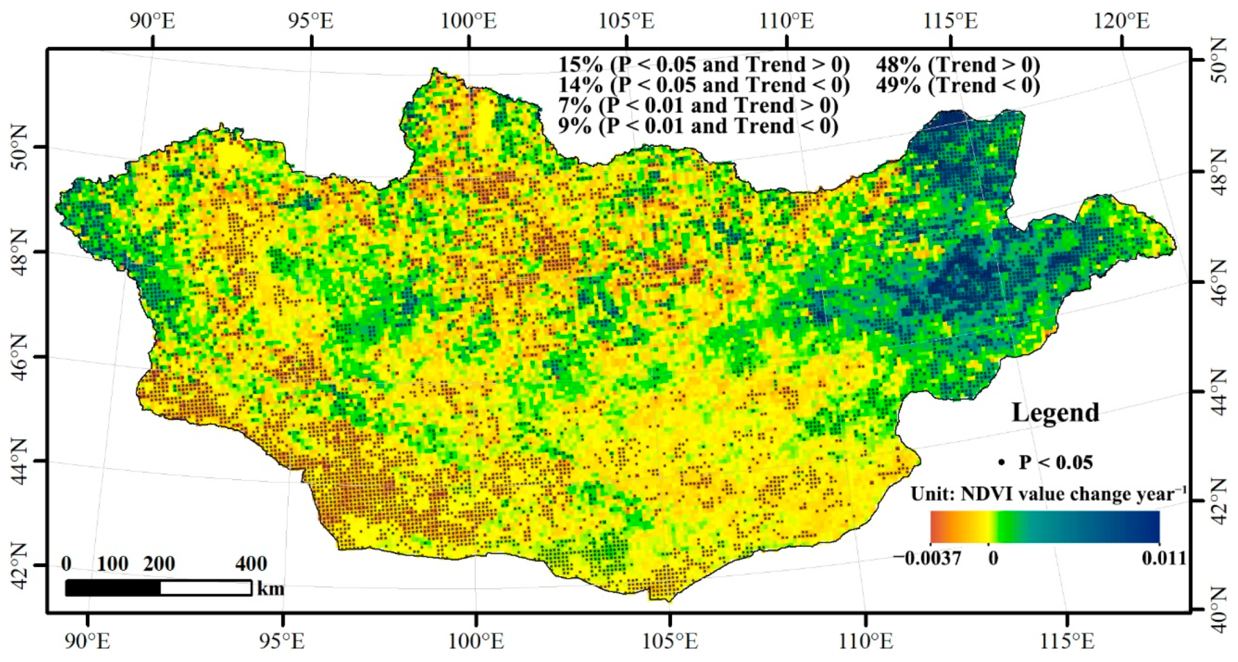
3.1. Dynamic Variation of NDVI

The proportion of NDVI change with an increasing trend (19%) from 1982 to 2015 approximately equaled the proportion with a decreasing trend (18%), although regional differences were found (Figure 3). The areas with significant variation in vegetation change were mainly located in eastern regions (Dornod and Sukhbaatar province), southern regions (Govi-Altai, south of Bayankhongor and west of Umnugovi province), western regions (Bayan-Ulgii province), and central regions (Arkhangai province) of Mongolia. Among these regions, the eastern and western regions showed a clear greening tendency. In contrast, the southern and central regions showed the greatest decrease.

The NDVI change trend varied among different types of vegetation in Mongolia from 1982 to 2015 and is shown in Figure 4. In this part of the analysis, we only counted those pixels that were statistically significant. For forest, pixels exhibiting an increasing trend and those with a decreasing trend occupied 17% and 15.4% of the total forest area, respectively, implying that these two trends each occurred over a similar areal extent. The highly significant (p < 0.01) and significant (0.01 < p < 0.05) trend of increasing and decreasing were also similar, indicating that the forest vegetation type in Mongolia showed no unified changing trend between 1982 and 2015.

For meadow steppe, areas with an increasing trend and those with a decreasing trend occupied 31.4% and 3% of the total steppe area, respectively, indicating that the area of Mongolian meadow steppe under an increasing trend was much higher than that under a decreasing trend. The area with a highly significant increasing trend was higher than that with a significant increasing trend. However, the area with a highly significant decreasing trend was lower than that with a significant decreasing trend. These findings suggest that meadow steppe in Mongolia went through a general positive development during 1982 to 2015.

For typical steppe, the proportion of pixels exhibiting an increasing trend and those with a decreasing trend were 17.1% and 9.9% of the whole typical steppe area, respectively, suggesting that the area under an increasing trend was higher than that under a decreasing trend during 1982–2015. The area with a highly significant increasing trend was lower than that with a significant increasing trend. In contrast, the area with a highly significant decreasing trend was higher than that with a significant decreasing trend. These findings imply that typical steppe in Mongolia has shown increased vegetation greening during this period. For desert steppe in Mongolia, the proportion of pixels exhibiting an increasing trend and decreasing trend were 5.6% and 12.4%, respectively, suggesting that the area under an increasing trend was much lower than that under a decreasing trend. Both the areas of highly significant increasing and decreasing trends were lower than those with a significant level, which implies that desert steppe in Mongolia showed vegetation degradation during this period.

For alpine steppe, the proportion of pixels exhibiting an increasing trend and decreasing trend were 26.3% and 5.8%, respectively, demonstrating that the area under an increasing trend was much higher than that under a decreasing trend. The areas of highly significant increasing and decreasing trends were lower than those with a significant trend, which implies that alpine steppe in Mongolia experienced increased greening during this period.

For Gobi Desert in Mongolia, the proportion of pixels exhibiting an increasing trend and decreasing trend were 8% and 35.1%, respectively, indicating that the area under an increasing trend was considerably lower than that under a decreasing trend during 1982–2015. The areas with highly significant increasing and decreasing trends were higher than those with a significant level, suggesting that Gobi Desert in Mongolia experienced a severe degradation process between 1982 and 2015.

In order to further understand the NDVI changes in Mongolia from 1982 to 2015, we focused on the relationships between the NDVI values at the beginning of the change and the variation within the 34-year period (Variation = Sen’s slope × 34). Figure 5a shows the scatter diagram of significant points (p < 0.05) calculated by the Sen’s slope method. The X-axis of Figure 5a reveals that the initial value range is between 0.05 and 0.95. However, based on the statistical results of the histogram of the initial value, the initial value of the changed region is mainly distributed within two levels: 0.05–0.2 and 0.3–0.5. From a spatial perspective, this indicates that the area of southern Mongolia containing Gobi Desert areas underwent major vegetation changes from 1982 to 2015. From the Y-axis, the variation is mainly distributed between −0.2 and 0.2, and the variation less than 0 (i.e., vegetation degradation) is mainly concentrated at −0.1 to 0. Combined with the specific spatial location, although the southern Gobi Desert region mainly reduced over the 34-year period, the spatial reduction was small and the amount of vegetation degradation was also small. However, from an ecosystem perspective, this degradation has a relatively large impact on the southern grassland ecosystem.

In Figure 5a, the variation count histogram reveals that, overall, the amount of vegetation increase was less than the amount of reduction. This contrasts with the areal analysis shown in Figure 3, in which the area of vegetation increase (15% of pixels) was larger than the area of reduction (14% of pixels). The distribution of reduction was wider (interval of 0–0.2), whereas the increase was more concentrated. The NDVI variation of different vegetation types is shown in Figure 5b. Meadow steppe, typical steppe, and alpine steppe vegetation types showed an increase, whereas the amount of variation in meadow steppe and desert steppe showed a decrease.

3.2. Trends of the Environmental Factors

The Sen’s slope and M-K test were applied to the 34-year period for the environmental factors including five climate factors and one human activity factor: precipitation, air temperature, wind speed, snow depth, specific humidity, and livestock quantity. The output of spatial distribution of these environmental factors’ trends and the corresponding areas were analyzed (Figure 6).

As demonstrated in Figure 6a, precipitation showed a high spatial heterogeneity of different trends across Mongolia. The slight increasing precipitation appeared in the north (Khuvsgul province) and south (Uvurkhangai province) of Mongolia with a rate of change of approximately 2 mm/a. The distinct decrease zones of precipitation were detected at the middle area (Ulaanbaatar, Khentii and Tuv province) of Mongolia, with rate of change of −4 mm/a. In general, most areas of Mongolia showed a decreasing trend in precipitation during 1982–2015 (Figure 6a).

In contrast, the temperature in Mongolia presented the opposite areal trend. As shown in Figure 6b, the temperature across Mongolia followed an observably increasing trend during 1982–2015, with no areas of decline. The highest temperature rise rate reached 0.06 °C/a, which is consistent with the results of previous studies [17]. The highest temperature increases were found in the southeast and northwest of Mongolia and the lowest temperature increases were found in the north and northeast boundary of Russia and Mongolia. Overall, Mongolia experienced a rapid and accelerated warming trend from 1982 to 2015.

Trends in wind speed factor also exhibited high spatial variability in Mongolia. As shown in Figure 6c, the largest increase and decrease were found at the northwest (Khovd, southern Zavkhan, and northern Govi-Altai province) and center (Uvurkhangai, Umnugovi, and Dornogovi province) of Mongolia, respectively, with an approximate trend of 0.015 m/s per year.

The snow depth of Mongolia mainly showed a positive trend (Figure 6d), with an increase rate of 7.6 mm/a. Few areas with a negative trend occurred across southeast and west Mongolia.

There was clear spatial trend distribution of specific humidity across Mongolia (Figure 6e). The specific humidity in the east of Mongolia generally decreased, whereas the specific humidity in the west area generally increased. The extreme values of these two trends were −20 and 13 mg/kg per year, respectively.

From 1982 to 2015, Mongolia experienced a considerable growth in livestock quantity. According to the National Statistical Office of Mongolia, livestock quantity increased substantially from 24.76 to 55.97 million during 1982–2015 and reached up to 66.21 million by 2018. From the perspective of spatial trend (Figure 6f), an overwhelming majority of city level showed a rapid increase in livestock quantity, and those with a relatively high positive trend were mainly found in the north-central and northeastern parts of Mongolia, with the increase rate of 15 thousand/a.

3.3. Relative Influences of Factors on Vegetation Distribution

3.3.1. Single Factor Influence Detection

The factor detector of GDM was used to reveal the driving force of each environmental factor on response variable NDVI. The higher the q value obtained from factor detector, the stronger the contribution of the factor to response variable. Moreover, the factor with maximum q value was defined as dominant. In this analysis, the response variable was taken as the annual average value of NDVI during 1982–2015. The climate factor and livestock quantity factor herein were also taken as annual averages for 1982–2015. All of the environmental factors and response variables are shown in Figure 6a. The results of the calculation of the q value of each environmental factor to NDVI are shown in

Table 3. The q value and p value of all factors for NDVI distribution and changes.

Factor	Prec	Vegett	Soilt	Snowd	Temp	Winds	Slopd	Livstq	Specfh	Elev	Curv	Slopa
Distribution	0.7811	0.7266	0.699	0.4879	0.4649	0.4504	0.2777	0.2054	0.1977	0.13	0.125	0.1073
p	0.000	0.000	0.000	0.000	0.000	0.000	0.000	0.000	0.000	0.000	0.000	0.000
Changes	0.0473	0.0984	0.098	0.0074	0.1232	0.0318	0.0135	0.122	0.1091	0.2026	0.0131	0.0206
p	0.000	0.000	0.000	0.020	0.000	0.000	0.003	0.019	0.000	0.000	0.000	0.000

. All factors were ranked in descending order by their dominant power as follows: Prec > Vegett > Soilt > Snowd > Temp > Winds > Slopd > Livstq > Specfh > Elev > Curv > Slopa (first row in Table 3).

Among the different environmental factors, the q values of precipitation, vegetation type, and soil type were the three largest factors (Table 3). Therefore, precipitation is the dominant factor affecting vegetation distribution in Mongolia. The q values of snow depth, temperature, and wind speed were 0.49, 0.46, and 0.45, respectively, and these together accounted for more than 40% of the NDVI distribution. However, the slope degree, specific humidity, elevation, curvature, and slope aspect affect the spatial distribution of hydrothermal conditions and thus affect the growth of vegetation. The influence of each factor is indirect and all q values for the NDVI distribution were below 20%, demonstrating that the factors of slope degree, specific humidity, elevation, curvature, and slope aspect had only a minimal influence on the NDVI distribution. Notably, the q value of human activity factor (livestock quantity) was 0.21, which indicates that grazing has little effect on the distribution of vegetation when considering Mongolia in its entirety. All driving factors of vegetation distribution test passed the significance test (p < 0.05)

3.3.2. Combined Influences Detection

The interaction between pairs of environmental factors (symbolized by ∩) was analyzed and the results are shown in

Table 4. Interaction detection between vegetation distribution and environmental factors.

C = q(X1 ∩ X2)	A = q(X1)	B = q(X2)	Conclusion	Interpretation
Prec ∩ ∩ Temp = 0.8049	0.7811	0.4649	C < A + B; C > A, B	↑
Prec ∩ Winds = 0.8387	0.7811	0.2937	C < A + B; C > A, B	↑
Prec ∩ Snowd = 0.8022	0.7811	0.4878	C < A + B; C > A, B	↑
Prec ∩ Specfh = 0.8217	0.7811	0.1976	C < A + B; C > A, B	↑
Prec ∩ Elev = 0.8264	0.7811	0.1299	C < A + B; C > A, B	↑
Prec ∩ Slopd = 0.8297	0.7811	0.2776	C < A + B; C > A, B	↑
Prec ∩ Slopa = 0.8187	0.7811	0.1072	C < A + B; C > A, B	↑
Prec ∩ Curv = 0.8054	0.7811	0.1250	C < A + B; C > A, B	↑
Prec ∩ Vegett = 0.8712	0.7811	0.7266	C < A + B; C > A, B	↑
Prec ∩ Soilt = 0.842	0.7811	0.6990	C < A + B; C > A, B	↑
Temp ∩ Winds = 0.5589	0.4649	0.2937	C < A + B; C > A, B	↑
Temp ∩ Snowd = 0.4949	0.4649	0.4878	C < A + B; C > A, B	↑
Temp ∩ Specfh = 0.5885	0.4649	0.1976	C < A + B; C > A, B	↑
Temp ∩ Elev = 0.5903	0.1619	0.1299	C < A + B; C > A, B	↑
Temp ∩ Slopd = 0.5447	0.4649	0.2776	C < A + B; C > A, B	↑
Temp ∩ Slopa = 0.5154	0.4649	0.1072	C < A + B; C > A, B	↑
Temp ∩ Curv = 0.4992	0.4649	0.1250	C < A + B; C > A, B	↑
Temp ∩ Vegett = 0.7648	0.4649	0.7266	C < A + B; C > A, B	↑
Temp ∩ Soilt = 0.7563	0.4649	0.6990	C < A + B; C > A, B	↑
Winds ∩ Snowd = 0.5912	0.2937	0.4878	C < A + B; C > A, B	↑
Winds ∩ Specfh = 0.3953	0.2937	0.1976	C < A + B; C > A, B	↑
Winds ∩ Elev = 0.4703	0.2937	0.1299	C > A + B; C > A, B	↑↑
Winds ∩ Slopd = 0.4803	0.2937	0.2776	C < A + B; C > A, B	↑
Winds ∩ Slopa = 0.4156	0.2937	0.1072	C < A + B; C > A, B	↑
Winds ∩ Curv = 0.3967	0.2937	0.1250	C > A + B; C > A, B	↑↑
Winds ∩ Vegett = 0.7683	0.2937	0.7266	C < A + B; C > A, B	↑
Winds ∩ Soilt = 0.5912	0.2937	0.6990	C < A + B; C > A, B	↑
Snowd ∩ Specfh = 0.6061	0.4878	0.1976	C < A + B; C > A, B	↑
Snowd ∩ Elev = 0.4703	0.2937	0.1299	C > A + B; C > A, B	↑↑
Snowd ∩ Slopd = 0.5722	0.4878	0.2776	C < A + B; C > A, B	↑
Snowd ∩ Slopa = 0.5439	0.4878	0.1072	C < A + B; C > A, B	↑
Snowd ∩ Curv = 0.5276	0.4878	0.1250	C < A + B; C > A, B	↑
Snowd ∩ Vegett = 0.777	0.4878	0.7266	C < A + B; C > A, B	↑
Snowd ∩ Soilt = 0.7665	0.4878	0.6990	C < A + B; C > A, B	↑
Specfh ∩ Elev = 0.4188	0.1976	0.1299	C > A + B; C > A, B	↑↑
Specfh ∩ Slopd = 0.5722	0.4878	0.2776	C < A + B; C > A, B	↑
Specfh ∩ Slopa = 0.5439	0.4878	0.1072	C < A + B; C > A, B	↑
Specfh ∩ Curv = 0.5276	0.4878	0.1250	C < A + B; C > A, B	↑
Specfh ∩ Vegett = 0.777	0.4878	0.7266	C < A + B; C > A, B	↑
Specfh ∩ Soilt = 0.7665	0.4878	0.6990	C < A + B; C > A, B	↑
Elev ∩ Slopd = 0.4185	0.1299	0.2776	C > A + B; C > A, B	↑↑
Elev ∩ Slopa = 0.1837	0.1299	0.1250	C < A + B; C > A, B	↑
Elev ∩ Curv = 0.2473	0.1299	0.1250	C < A + B; C > A, B	↑
Elev ∩ Vegett = 0.7572	0.1299	0.7266	C < A + B; C > A, B	↑
Elev ∩ Soilt = 0.7819	0.1299	0.6990	C < A + B; C > A, B	↑
Slopd ∩ Slopa = 0.2881	0.2776	0.1072	C < A + B; C > A, B	↑
Slopd ∩ Curv = 0.2867	0.2776	0.1250	C < A + B; C > A, B	↑
Slopd ∩ Vegett = 0.763	0.2776	0.7266	C < A + B; C > A, B	↑
Slopd ∩ Soilt = 0.7556	0.2776	0.6990	C < A + B; C > A, B	↑
Slopd ∩ Curv = 0.1686	0.1072	0.1250	C < A + B; C > A, B	↑
Slopd ∩ Vegett = 0.7453	0.1072	0.7266	C < A + B; C > A, B	↑
Slopd ∩ Soilt = 0.746	0.1072	0.6990	C < A + B; C > A, B	↑
Curv ∩ Vegett = 0.7422	0.1250	0.7266	C < A + B; C > A, B	↑
Curv ∩ Soilt = 0.746	0.1250	0.6990	C < A + B; C > A, B	↑
Vegett ∩ Soilt = 0.8414	0.7266	0.6990	C < A + B; C > A, B	↑

Note: “↑” and “↑↑” refer to X1 ∩ X2 enhancing each other and X1 ∩ X2 nonlinear enhancement, respectively.

, including comparison of their interactive q value and individual q value to NDVI. The top five interactive q values decreased in the following order: Prec ∩ Vegett > Prec ∩ Soilt > Vegett ∩ Soilt > Prec ∩ Winds > Prec ∩ Slopd. This indicates that the interactions between meteorological factors (precipitation or wind speed), vegetation type, soil type, and topography had the greatest impact on the NDVI value. Two factors exhibiting a nonlinear enhancement after the interaction means that the q value after interaction is greater than the sum of the individual q values before interaction (q(X1 ∩ X2) > q(X1) + q(X2)). In this study, factors that showed nonlinear enhancement after interaction included Snowd ∩ Elev, Specfh ∩ Slopd, Winds ∩ Elev, Specfh ∩ Elev, Elev ∩ Slopd, Winds ∩ Curv, Specfh ∩ Curv and Specfh ∩ Slopa. This indicates that the influence of topographic factors (Elev, Slopd, Slopa, and Curv) as indirect factors on vegetation growth are mainly reflected in the interaction with other factors. For example, when interacting with meteorological factors, topographic factors can markedly enhance their single effects on the NDVI value. Naturally, all interactive q values of pairs of environmental factors were larger than any q values of an individual factor, indicating that the effects of environmental factors on the distribution of NDVI are not independent but interactive. Compared with these factors that enhanced each other, the correlation between these nonlinear enhancement factors is relatively low (Table 4).

3.3.3. Optimal Range of Factors for NDVI Detection

Using the risk detector of GDM, the optimal range results for the main environmental factors are shown in

Table 5. The optimal range of each environmental factors with maximum NDVI.

Factor	Optimal Range	Mean Value of NDVI
Prec (mm)	331–696	0.6811
Temp (°C)	−12.5–0	0.4903
Windv (m/s)	2.74–3.27	0.5591
Snowd (mm)	92–94	0.5948
Specfh (mg/kg)	4.51–5.25	0.5381
Elev (m)	535–974	0.4991
Slopd (°)	4.0–23.8	0.5276
Slopa (°)	330–360	0.4355
Curv	−0.62–0.08	0.4909
Vegett	Forest	0.4963
Soilt	Pine sandy soil	0.777
Livstq	128,197–132,676	0.6287

. We assumed the limits of environmental factors with the biggest average value of NDVI is the optimal range for vegetation growth. There was a range of different relationships between different factors and the vegetation distribution. For example, there was a positive correlation between precipitation and NDVI value, indicating that the annual average NDVI value increased with the increasing precipitation. In this study, when the annual precipitation was between 331 mm and 596 mm, the annual average NDVI value reached maximum. In contrast, the NDVI increased with decreasing temperature and the maximum NDVI value appeared in the first stratum (stratum for minimum temperature) of temperature.

Only monotonic relationships were found between precipitation, temperature, and vegetation growth; other factors were non-monotonic. For instance, the second stratum of wind speed (2.74–3.27 m/s) contained the maximum NDVI, implying that this stratum of wind speed promoted widespread vegetation growth in Mongolia. As for snow depth, the maximum annual average NDVI value appeared in the stratum between 92 mm and 94 mm, implying that this stratum was the optimum for vegetation growth. The maximum annual NDVI value of 0.49 roughly corresponded to an altitude between 535 m and 974 m. We also found that NDVI values can reach the peak value when the stratum of specific humidity is between 4.51 mg/kg and 5.25 mg/kg. As for slope degree, slope aspect, and curvature, the optimal range of these factors were 4.1–23.8°, 330–360°, and −0.62–0.08, for which the NDVI can reach 0.53, 0.43, and 0.49, respectively. For the vegetation types, the highest NDVI value was found for the forest, followed by meadow steppe. For the soil types, the highest NDVI value was found for the pine sandy soil, followed by mountain peat soil and grey forest soil, in which all the average NDVI values exceeded 0.70. For livestock quantity, the NDVI peak occurred in the stratum between 128,000 and 132,000. These findings could play a guiding role in restoring vegetation engineering in arid land. The detection results of the dominant range of environmental factors in this study reveal the dominant habitat range for vegetation growth, which can help land managers in planning a suitable range of vegetation growth environment. It also plays the role of planting grass or cash crops as much as possible with the minimum human intervention. In short, the detection results of the dominant range of environmental factors can provide a basic environmental framework for vegetation growth.

3.3.4. Significant Differences between Factors

The significant differences between the effects of environmental factors on vegetation growth from the ecological detector in GDM are shown in

Table 6. Statistical significance of the detection factors (95% confidence level).

Factor	Prec	Soilt	Snowd	Temp	Winds	Vegett	Slopd	Specfh	Elev	Cuve	Slopa
Prec	/
Soilt	Y	/
Snowd	Y	Y	/
Temp	Y	Y	N	/
Winds	Y	Y	Y	Y	/
Vegett	Y	Y	Y	Y	Y	/
Slopd	Y	Y	Y	Y	N	Y	/
Specfh	Y	Y	Y	Y	Y	Y	Y	/
Elev	Y	Y	Y	Y	Y	Y	Y	Y	/
Cuve	Y	Y	Y	Y	Y	Y	Y	Y	N	/
Slopa	Y	Y	Y	Y	Y	Y	Y	Y	N	N	/

Note: “Y” and “N” refer to whether there is Yes or No significant difference between two factors.

. The topographical elevation, slope degree, and slope aspect all had the same influence on vegetation growth. In contrast, for the slope degree and snow depth factor, only wind speed and temperature factors had no significant effect on the spatial distribution of vegetation, respectively. There were significant differences between all of the other environmental factors.

3.4. Relative Influences of Factors on Vegetation Changes

3.4.1. Single Factor Influence Detection

Using the annual average NDVI value as the response variable, the annual average climate factors and the topographical factors, as well as the livestock quantity as environmental variables to explore their internal relationships is inclined to reveal the physical mechanism between them. Therefore, we used the Sen’s slope method to obtain the time series change trend of NDVI and environmental factors, and then used the GDM to detect the relationships between their changes. All these slope variables are shown in Figure 3 and Figure 6. Note that only six factors changed over time, including five climatic factors and the livestock quantity factor. In order to ensure a complete contrast, the invariant factors (i.e., topographical factors, vegetation type, and soil type) were also included in the model calculations.

The results of the factor detector changes in GDM are shown in Figure 7a (blue curve) and Table 3 (the second row). All factors were ranked in descending order by their dominant power: Elev (0.2026) > Temp (0.1232) > Livstq (0.122) > Specfh (0.1091) > Vegett (0.0984) > Soilt (0.098) > Prec (0.0473) > Winds (0.0318) > Slopa (0.0206) > Slopd (0.0135) > Curv (0.0131) > Snowd (0.0074), indicating that vegetation changes during 1982–2015 were mainly due to changes of elevation and temperature, rather than the precipitation and vegetation type which are the dominant controlling factors on vegetation distribution. Furthermore, changes in livestock quantity ranked third in terms of influence on vegetation changes, but eighth for its influence on vegetation distribution. For Mongolia as a whole, the effects of these factors on the vegetation change were minimal (all the q values were less than 0.21), indicating that the changes of environmental factors do not match the changes of vegetation very well in terms of spatial distribution across Mongolia. This is because the physical mechanism is complicated and spatial heterogeneity is ignored when regarding the entirety of Mongolia as a single research area. This may lead to misunderstanding of the analysis results. However, our study uses vegetation types as the basic unit to explore the spatial and temporal characteristics of NDVI changes and the corresponding drivers, which are more in line with the natural geographical law. Therefore, our statistical results can approximately reveal the relative influence power between factors on vegetation changes and could be used as a reference with which to compare the contributions of different factors.

3.4.2. Vegetation Change Drivers under Different Vegetation Types

Since the analysis of the whole of Mongolia as a research area ignores its spatial heterogeneity, we used a partitioning approach to separately analyze which environmental factors drive vegetation changes and thus provide a more accurate assessment of the rate of change between vegetation and environmental factors. In this section, we detected factors based on the six different vegetation types (Figure 2k). The results of factor detection are shown in Figure 7b.

For forest, the maximum q value was for livestock quantity (q = 0.5), followed by elevation (q = 0.22) and wind speed (q = 0.17). Similarly, for meadow steppe, the dominant factor was livestock quantity (q = 0.53), followed by elevation (q = 0.37) and precipitation (q = 0.31). For the typical steppe, the dominant factor was elevation (q = 0.26) and the secondary driver was soil type (q = 0.17). For the desert steppe, the main influencing factor was also the livestock quantity (q = 0.27). The contribution power of elevation and specific humidity were 0.19 and 0.13, respectively. For Alpine steppe, the dominant factor was slope aspect, for which the q value could reach 0.46. In addition, other factors also had high driving force values, such as elevation (q = 0.43), temperature (q = 0.39), and slope degree (q = 0.33), indicating that these factors have major impact on vegetation changes. For Gobi Desert, as shown in Figure 7b, the dominant factor was again livestock quantity (q = 0.44). However, the remaining factors such as precipitation (q = 0.15) and wind speed (q = 0.14) showed a weak influence on vegetation changes. Overall, based on the analysis of different vegetation types, the dominant factors that affect vegetation change were livestock quantity and topographical factor.

4. Discussion

The analysis of the driving factors and trends of vegetation growth and vegetation changes derived from satellite observations are of great importance for evaluating the value of grassland ecosystems in Mongolia. However, a major challenge remaining for research into the driving force of vegetation growth and changes in Mongolia is that analytical models or methods fail to take the spatial heterogeneity of variables into account. In this study, we used Sen’s slope and the M-K test to allow trend analysis of vegetation changes. These two pixel-based analysis methods can be used to delve into spatial heterogeneity information of vegetation changes. Then, the GDM based on spatial stratified heterogeneity [48], was utilized to investigate the driving force of vegetation growth and changes.

4.1. The Trend of Vegetation Changes

Bao et al. [21] used the GIMMS NDVI to study the vegetation dynamics in Mongolia, and found that different vegetation types had different variation trends, but only the forest and alpine steppe exhibited a significant increasing trend and the meadow steppe, typical steppe, and desert steppe exhibited no significant trend. The trend of vegetation changes in this study revealed that the meadow steppe, typical steppe, and alpine steppe exhibited an increasing trend; the desert steppe and the Gobi Desert showed a significant decreasing trend; and only the forest showed no significant trend (Table 1). Tsydypov et al. [22] also found that the variation of the Gobi Desert NDVI decreased in Mongolia and there was a trend of xerophytization had already been occurring in the sparse vegetation of the Gobi Desert. Bao et al. [21] utilized the least-squares linear regression model, and in this study, all pixels of the same vegetation type were included, without considering the spatial heterogeneity of the vegetation changes. We suggest that this is the main reason for the difference in trend results. Global warming has been observed in different studies with different data sources [50,51,52]. According to the records at 48 meteorological stations in Mongolia, Dagvadorj et al. [17] showed that the annual mean temperature of Mongolia increased by 0.062 °C during 1981–2006, which is in agreement with our study. Moreover, Dagvadorj et al. [17] observed that precipitation showed a downward trend, which was also supported by our results. The results of vegetation trend in our findings are different from Zhao et al. [53], as they showed that the NDVI has not shown a persistent increase after 1998, thus causing an insignificant trend over the entire study period from 1982 to 2011. This discrepancy might be caused by the reason that Zhao et al. [53] analyzed the entire Mongolia as a whole to explore the trends of vegetation changes but did not detect the trends by partitioned areas.

4.2. Driving Force of Vegetation Distribution and Changes

Several studies have shown that Mongolian vegetation is particularly sensitive and susceptible to climate change and human activity [21,22,23]. Moreover, the spatial distribution of climate factors in Mongolia is mainly because of the combined effects of latitude, topography, and monsoon effects. In this study, we found a significant positive correlation between the spatial distribution of vegetation and the precipitation, which is consistent with the study of Bao et al. [21], Gantsetseg et al. [54], Filei et al. [23], and Zhao et al. [53]. Furthermore, vegetation type and soil type are the main factors affecting vegetation distribution. Note that different vegetation types have different NDVI values. The relationship between soil and vegetation distribution is relatively complicated. From the perspective of soil genesis, the effects of soil on vegetation distribution cannot be simply determined because vegetation also has a transformation effect on soil and different NDVI values (different vegetation types) have different effects on soil transformation [55]. Therefore, there is a relatively strong interaction between soil type and vegetation distribution. Related studies have also shown that when precipitation is the dominant factor, soil type has an important impact on vegetation growth and rainwater reuse [6,56].

Taking the whole of Mongolia as the study area, the influence (q value) of environmental factors on vegetation changes is small. This is because we ignored the spatial heterogeneity of vegetation changes. Therefore, we separately detected the driving force of different vegetation types for their changes during 1982–2015. The results show that grazing was the dominant factor leading to changes in forest, meadow steppe, desert steppe, and Gobi Desert. This indicates that overgrazing had the strongest influence on most of Mongolia’s vegetation changes over the studied period. In contrast, for the typical steppe and alpine steppe, topographical factors were dominant because the topography plays an important role in the redistribution of water resources and solar energy resources. For example, the photosynthesis of sunny slope vegetation is stronger than that of shady slopes, and the evapotranspiration of shady slope vegetation is weaker than that of vegetation growing on sunny slopes. Quantifying the driving factors of vegetation distribution has great guiding significance for agricultural site selection. The factor ranking results can provide more accurate factor weight information. In process of constructing the agricultural location model, it can help researchers to assign reasonable weight values to each factor [57].

4.3. Optimal Range of Vegetation Growth

Quantification of the optimal range of environmental factors for vegetation distribution in a region helps decision makers to take appropriate interventions to restore vegetation and improve the ecological environment. In GDM, optimal range information is generated from the strata. The division of this strata is a part of the data preprocessing step. When the environmental factor is the continuous numerical data (e.g., precipitation or temperature), the first step is to discretize the environmental factor into strata. The choice of an appropriate discretization method is important because discrete results can directly affect the subsequent GDM results. Many studies recommend using the largest q value as the optimal discretization criterion [58,59]. Therefore, in our study, we used the maximum q value as a criterion function to find the optimal layering method, ensuring the optimal range.

Due to the interaction between the factors, the optimal range of one environmental factor for vegetation growth cannot be considered separately. For example, in current study, the range −12–0 °C was taken as the suitable limit of temperature factor for vegetation growth, however, this range was obtained by combining the temperature with the precipitation and topography factors. The northern part of Mongolia is mainly affected by the airflow of the Arctic Ocean. In addition, the terrain is undulating, and the precipitation is relatively high, causing the dense vegetation. However, because of the high latitude and altitude, the temperature in this area is lower than that of the southern area. The optimal temperature range −12–0 °C for vegetation growth might only reflect the annual average temperature in the northern part of Mongolia.

4.4. Relative Degree of Vegetation Changes

The initial value of NDVI can reflect the vegetation coverage at the beginning of vegetation change (i.e., 1982 in this study). Changes in the NDVI are often used as indicators of the degree of desertification development. However, many studies on this aspect only focus on the trend of vegetation change and rarely pay attention to the state of the region before the change [23,60]. To assess the degree of vegetation changes, not only do we need to obtain the trends and the amount of vegetation change, we also need to take the initial state of the vegetation into account. For example, in this study, the NDVI decrease in the Gobi Desert region was between 0 and 0.1 during 1982–2015. However, we should consider that the vegetation index value in this area before the decline was between 0 and 0.2 (initial value).

4.5. Caveats of Our Study

Our study is subject to a few caveats. First, we derived the NDVI values from NOAA/AVHRR GIMMS NDVI3g dataset (1/12° and bimonthly frequency, spanning 1982–2015) to explore vegetation distribution and changes. For current study, the spatial resolutions are relatively coarse. As large spatial scale NDVI over heterogeneous surfaces is easily susceptible to soil background in low-vegetated areas and saturated in well-vegetated areas. There are some subsequent vegetation indices to improve it, for example, Enhanced Vegetation Index (EVI) [61] and Soil Adjusted Vegetation Index (SAVI) [62,63]. In addition, biomass estimation can also be used as a good indicator of vegetation conditions. For example, Otgonbayar et al. [64] has estimated pasture biomass in Mongolia using partial least squares, random forest regression, and Landsat 8 imagery. However, considering data availability, this GIMMS NDVI3g dataset is still likely the best one we can currently use for a long time series vegetation analysis. For example, although EVI and SAVI can be derived from a MODIS dataset with higher spatial resolution, MODIS datasets cover a relatively short period of time only since 2000 [65]. Furthermore, long time series vegetation analysis can delve into more objective vegetation change trend information and improve the robustness of analysis results. For vegetation trend research, previous research has shown that the trends of NDVI changes obtained by Landsat (30 m), MODIS (1 km), and AVHRR (8 km) are not significantly different [66].

Second, we used climate data from the Global Land Data Assimilation System (GLDAS) Catchment Land Surface Model (0.25° × 0.25° spatial resolution), which also seem relatively coarse, especially for north of Mongolia (mountainous areas). Obviously, some meteorological data with high temporal-spatial resolution and high quality have been developed in Mongolia, such as average monthly air temperature over Mongolia (spanning 2002–2017) estimated by Otgonbayar et al. [67] using MODIS land surface temperature (LST) time series and machine learning techniques. However, considering the requirement that the meteorological factors have to be resampled to match the spatial resolution of the NDVI data, the GLDAS dataset is a better choice to meet this requirement. In addition, our model results were executed with data at coarse spatial and temporal scales, which possibly result in the potential scale dependence of the model results. However, we are tracing each pixel to calculate the spatial and temporal characteristics of NDVI changes and the corresponding drivers. Additionally, for such study of macro-scale vegetation changes and driving forces, with the improvement of data resolution, the marginal benefits are gradually decreasing. More in-depth research should be further examined on the scale dependence of the trends of NDVI changes.

5. Conclusions

Based on the GIMMS AVHRR NDVI3g datasets from 1982 to 2015, five climatic data sets (precipitation, air temperature, specific humidity, wind speed, and snow depth) of different time series, four topographical data sets (elevation, curvature, slope degree, and slope aspect), vegetation type data, soil type data, and livestock quantity information, the spatial and temporal distribution characteristic of NDVI changes, the driving force detection of NDVI distribution and changes, the interaction of different environmental factors on vegetation growth, and the optimal range of environmental factors for vegetation growth were analyzed in Mongolia from 1982 to 2015.

On the whole, the area showing a downward trend (accounts for 15% of the total area) was basically equal to the area showing an upward trend (accounts for 14% of the total area) of vegetation variation in Mongolia. However, there was significant heterogeneity between different vegetation types. The meadow steppe, typical steppe, and alpine steppe of Mongolia mainly showed a clear greening tendency, whereas the desert steppe and Gobi Desert showed a degradation tendency.

We found that precipitation, vegetation type, and soil type were the dominant factors influencing NDVI distribution across the whole of Mongolia. The interaction between each pair of factors manifested as mutual enhancement and nonlinear enhancement. Among these environmental factors, topographical factors and climatic factors were most likely to result in nonlinear enhancement effects. This confirms that environmental factors interacted to influence the distribution of NDVI, and interaction between environmental factors plays a more vital role than the influence of the individual one on vegetation growth.

Revealing the optimal range of key environmental factors on vegetation growth is equivalent to clarify the ecological niche of vegetation growth in a study area, facilitating ecological protection and vegetation restoration, and alleviating desertification problems in semi-arid and arid regions. For example, in this study, the results showed that when the annual precipitation is between 331 mm and 596 mm, forest vegetation type and pine sandy soil type could generate the maximum NDVI value in Mongolia.

We stress that the obtained relationships between the environmental factors and vegetation growth are only statistical relationships, rather than causal relationships. However, the results of statistical analysis are often the forerunners of the physical mechanism analysis between geographical elements. Therefore, the results of this study are still instructive to Mongolia’s response to climate change in the process of ecological construction and animal husbandry development.

References

1. Gottfried, M.; Pauli, H.; Futschik, A.; Akhalkatsi, M.; Barančok, P.; Benito Alonso, J.L.; Coldea, G.; Dick, J.; Erschbamer, B.; Fernández Calzado, M.A.R.; et al. Continent-wide response of mountain vegetation to climate change. Nat. Clim. Chang. 2012, 2, 111–115. [Google Scholar] [CrossRef]
2. Gong, Z.; Zhao, S.; Gu, J. Correlation analysis between vegetation coverage and climate drought conditions in North China during 2001–2013. J. Geogr. Sci. 2017, 27, 143–160. [Google Scholar] [CrossRef]
3. Parmesan, C.; Yohe, G. A globally coherent fingerprint of climate change impacts across natural systems. Nature 2003, 421, 37–42. [Google Scholar] [CrossRef] [PubMed]
4. Zhao, J.; Du, Z.; Wu, Z.; Zhang, H.; Guo, N.; Ma, Z.; Liu, X. Seasonal variations of day-and nighttime warming and their effects on vegetation dynamics in China’s temperate zone. Acta Ecol. Sin. 2018, 73, 395–404. [Google Scholar] [CrossRef]
5. Du, Z.; Zhang, X.; Xu, X.; Zhang, H.; Wu, Z.; Pang, J. Quantifying influences of physiographic factors on temperate dryland vegetation, Northwest China. Sci. Rep. 2017, 7. [Google Scholar] [CrossRef] [PubMed]
6. Piao, S.; Mohammat, A.; Fang, J.; Cai, Q.; Feng, J. NDVI-based increase in growth of temperate grasslands and its responses to climate changes in China. Glob. Environ. Chang. 2006, 16, 340–348. [Google Scholar] [CrossRef]
7. Zhao, L.; Dai, A.; Dong, B. Changes in global vegetation activity and its driving factors during 1982–2013. Agric. For. Meteorol. 2018, 249, 198–209. [Google Scholar] [CrossRef]
8. Chen, S.; Gan, T.Y.; Tan, X.; Shao, D.; Zhu, J. Assessment of CFSR, ERA-Interim, JRA-55, MERRA-2, NCEP-2 reanalysis data for drought analysis over China. Clim. Dyn. 2019, 53, 737–757. [Google Scholar] [CrossRef]
9. Guo, J.T.; Hu, Y.M.; Xiong, Z.; Yan, X.L.; Ren, B.H.; Bu, R.C. Spatiotemporal variations of growing-season NDVI and response to climate change in permafrost zone of Northeast China. Chin. J. Appl. Ecol. 2017, 28, 2413–2422. [Google Scholar] [CrossRef]
10. Baniya, B.; Qiuhong, T. Vegetation dynamics in response to climate change based on satellite derived NDVI in Nepal. EGU Gen. Assem. Conf. Abstr. 2018, 20, 91. [Google Scholar]
11. Peng, J.; Liu, Z.; Liu, Y.; Wu, J.; Han, Y. Trend analysis of vegetation dynamics in Qinghai–Tibet Plateau using Hurst Exponent. Ecol. Indic. 2012, 14, 28–39. [Google Scholar] [CrossRef]
12. Hein, L.; de Ridder, N.; Hiernaux, P.; Leemans, R.; de Wit, A.; Schaepman, M. Desertification in the Sahel: Towards better accounting for ecosystem dynamics in the interpretation of remote sensing images. J. Arid Environ. 2011, 75, 1164–1172. [Google Scholar] [CrossRef]
13. Goodchild, M.F. The Validity and Usefulness of Laws in Geographic Information Science and Geography. Ann. Assoc. Am. Geogr. 2004, 2, 300–303. [Google Scholar] [CrossRef] [Green Version]
14. Fischer, M.; Wang, J. Spatial Data Analysis: Models, Methods and Techniques; Springer: Berlin/Heidelberg, Germany, 2011. [Google Scholar] [CrossRef]
15. Fortin, M.J. Spatio-Temporal Heterogeneity: Concepts and Analyses by Pierre R.L. Dutilleul. Q. Rev. Biol. 2012, 87. [Google Scholar] [CrossRef]
16. Wang, J.; Li, X.; Christakos, G.; Liao, Y.; Zhang, T.; Gu, X.; Zheng, X.Y. Geographical Detectors-ased Health Risk Assessment and its Application in the Neural Tube Defects Study of the Heshun Region, China. Int. J. Geogr. Inf. Sci. 2010, 24, 107–127. [Google Scholar] [CrossRef]
17. Dagvadorj, D.; Natsagdorj, L.; Dorjpurev, J.; Namkhainyam, B. Mongolia Assessment Report on Climate Change 2009. Minist. Nat. Environ. Tour. Ulaanbaatar 2009, 2, 34–46. [Google Scholar]
18. Jiang, L.; Yao, Z.; Huang, H.Q. Climate variability and change on the Mongolian Plateau: Historical variation and future predictions. Clim. Res. 2016, 67, 1–14. [Google Scholar] [CrossRef]
19. Hilker, T.; Natsagdorj, E.; Waring, R.H.; Lyapustin, A.; Wang, Y. Satellite observed widespread decline in Mongolian grasslands largely due to overgrazing. Glob. Chang. Biol. 2014, 20, 418–428. [Google Scholar] [CrossRef] [Green Version]
20. John, R.; Chen, J.; Kim, Y.; Ou-yang, Z.; Xiao, J.; Park, H.; Shao, C.; Zhang, Y.; Amarjargal, A.; Batkhshig, O.; et al. Differentiating anthropogenic modification and precipitation-driven change on vegetation productivity on the Mongolian Plateau. Landsc. Ecol. 2016, 31, 547–566. [Google Scholar] [CrossRef]
21. Bao, G.; Bao, Y.; Sanjjava, A.; Qin, Z.; Zhou, Y.; Xu, G. NDVI-indicated long-term vegetation dynamics in Mongolia and their response to climate change at biome scale. Int. J. Climatol. 2015, 35, 4293–4306. [Google Scholar] [CrossRef]
22. Tsydypov, B.Z.; Garmaev, E.Z.; Tulokhonov, A.K.; Batotsyrenov, E.A.; Ayurzhanaev, A.A.; Alymbaeva, Z.B.; Chimeddorj, T. Degradation of the Vegetation Cover in Central Mongolia: A Case Study. J. Resour. Ecol. 2015, 6, 73–78. [Google Scholar] [CrossRef]
23. Filei, A.A.; Slesarenko, L.A.; Boroditskaya, A.V.; Mishigdorj, O. Analysis of Desertification in Mongolia. Russ. Meteorol. Hydrol. 2018, 43, 599–606. [Google Scholar] [CrossRef]
24. Zhou, X.; Yamaguchi, Y.; Arjasakusuma, S. Distinguishing the vegetation dynamics induced by anthropogenic factors using vegetation optical depth and AVHRR NDVI: A cross-border study on the Mongolian Plateau. Sci. Total Environ. 2018, 616, 730–743. [Google Scholar] [CrossRef] [PubMed]
25. Klinge, M.; Dulamsuren, C.; Erasmi, S.; Karger, D.N.; Hauck, M. Climate effects on vegetation vitality at the treeline of boreal forests of Mongolia. Biogeosciences 2018, 15, 1319–1333. [Google Scholar] [CrossRef] [Green Version]
26. Tian, F.; Fensholt, R.; Verbesselt, J.; Grogan, K.; Horion, S.; Wang, Y. Evaluating temporal consistency of long-term global NDVI datasets for trend analysis. Remote Sens. Environ. 2015, 163, 326–340. [Google Scholar] [CrossRef]
27. Jiapaer, G.; Liang, S.; Yi, Q.; Liu, J. Vegetation dynamics and responses to recent climate change in Xinjiang using leaf area index as an indicator. Ecol. Indic. 2015, 58, 64–76. [Google Scholar] [CrossRef]
28. Wang, T. Vegetation NDVI Change and Its Relationship with Climate Change and Human Activities in Yulin, Shaanxi Province of China. J. Geosci. Environ. Prot. 2016, 4, 28–40. [Google Scholar] [CrossRef] [Green Version]
29. Leroux, L.; Bégué, A.; Lo Seen, D.; Jolivot, A.; Kayitakire, F. Driving forces of recent vegetation changes in the Sahel: Lessons learned from regional and local level analyses. Remote Sens. Environ. 2017, 191, 38–54. [Google Scholar] [CrossRef] [Green Version]
30. Jinkai, L.; Dengfeng, L.; Qiang, H.; Jiuliang, F.; Mu, L.; Guobao, L. Analysis of the spatial-temporal change and impact factors of the vagetation index in Yulin, Shaanxi Province, in the last 17 years. Acta Ecol. Sin. 2018, 38. [Google Scholar] [CrossRef]
31. Bespalov, N.D.; Gourevitch, A. Soils of Outer Mongolia (Mongolian People’s Republic); Israel Program for Scientific Translations: Jerusalem, Israel, 1964. [Google Scholar]
32. Pinzon, J.; Tucker, C. A Non-Stationary 1981–2012 AVHRR NDVI3g Time Series. Remote Sens. 2014, 6, 6929–6960. [Google Scholar] [CrossRef] [Green Version]
33. Garonna, I.; de Jong, R.; de Wit, A.J.W.; Mücher, C.A.; Schmid, B.; Schaepman, M.E. Strong contribution of autumn phenology to changes in satellite-derived growing season length estimates across Europe (1982–2011). Glob. Chang. Biol. 2014, 20, 3457–3470. [Google Scholar] [CrossRef] [PubMed]
34. HOLBEN, B.N. Characteristics of maximum-value composite images from temporal AVHRR data. Int. J. Remote Sens. 1986, 7, 1417–1434. [Google Scholar] [CrossRef]
35. Rodell, M.; Houser, P.; Jambor, U.; Gottschalck, J.; Mitchell, K.; Meng, J.; Arsenault, K.; Brain, C.; Radakovich, J.; MG, B.; et al. The Global Land Data Assimilation System. Bull. Amer. Meteor. Soc. 2004, 85, 381–394. [Google Scholar] [CrossRef] [Green Version]
36. Cheng, S.; Guan, X.; Huang, J.; Ji, M. Analysis of Response of Soil Moisture to Climate Change in Semi-arid Loess Plateau in China Based on GLDAS Data. J. Arid Meteorol. 2013, 27, 4–19. [Google Scholar] [CrossRef]
37. Tao, J.; Reichle, R.H.; Koster, R.D.; Forman, B.A.; Xue, Y. Evaluation and Enhancement of Permafrost Modeling with the NASA Catchment Land Surface Model. J. Adv. Model. Earth Syst. 2017, 9, 2771–2795. [Google Scholar] [CrossRef] [Green Version]
38. Ouma, Y.O.; Aballa, D.O.; Marinda, D.O.; Tateishi, R.; Hahn, M. Use of GRACE time-variable data and GLDAS-LSM for estimating groundwater storage variability at small basin scales: A case study of the Nzoia River Basin. Int. J. Remote Sens. 2015, 36, 5707–5736. [Google Scholar] [CrossRef]
39. Jarvis, A.; Reuter, H.; Nelson, A.; Guevara, E. Ole-Filled Seamless SRTM Data V4; International Centre for Tropical Agriculture (CIAT): Cali, Colombia, 2008. [Google Scholar]
40. Dorijgotov, D. National Atlas of Mongolia; Institute of Geography, Ulaanbaatar City: Ulaanbaatar, Mongolia, 2009. [Google Scholar]
41. Sen, P.K. Estimates of the Regression Coefficient Based on Kendall’s Tau. J. Am. Stat. Assoc. 1968, 63, 1379–1389. [Google Scholar] [CrossRef]
42. Mann, H. Non-Parametric Test against Trend. Econometrica 1945, 13, 245–259. [Google Scholar] [CrossRef]
43. Kendall, M. Rank Correlation Methods; Griffin: London, UK, 1975. [Google Scholar]
44. Rahman, A.; Dawood, M. Satio-statistical analysis of temperature fluctuation using Mann-Kendall and Sen’s slope approach. Clim. Dyn. 2017, 48, 783–797. [Google Scholar] [CrossRef]
45. Alhaji, U.; Yusuf, A.; Edet, C.; Oche, C.; Agbo, E. Trend Analysis of Temperature in Gombe State Using Mann Kendall Trend Test. J. Sci. Res. Rep. 2018, 20. [Google Scholar] [CrossRef]
46. Ali, R.; Kuriqi, A.; Abubaker, S.; Kisi, O. Long-Term Trends and Seasonality Detection of the Observed Flow in Yangtze River Using Mann-Kendall and Sen’s Innovative Trend Method. Water 2019, 11, 1855. [Google Scholar] [CrossRef] [Green Version]
47. Kamal, N.; Pachauri, S. Mann-Kendall, and Sen’s Slope Estimators for Precipitation Trend Analysis in North-Eastern States of India. Int. J. Comp. Appl. 2019, 177, 7–16. [Google Scholar] [CrossRef]
48. Wang, J.; Zhang, T.; Fu, B. A measure of spatial stratified heterogeneity. Ecol. Indic. 2016, 67, 250–256. [Google Scholar] [CrossRef]
49. Jenks, G. The Data Model Concept in Statistical Mapping. Int. Yearb. Cartogr. 1967, 7, 186–190. [Google Scholar]
50. Zhu, Z.; Piao, S.; Myneni, R.B.; Huang, M.; Zeng, Z.; Canadell, J.G.; Ciais, P.; Sitch, S.; Friedlingstein, P.; Arneth, A.; et al. Greening of the Earth and its drivers. Nat. Clim. Chang. 2016, 6, 791–795. [Google Scholar] [CrossRef]
51. Vinnikov, K.Y.; Robock, A.; Stouffer, R.J.; Walsh, J.E.; Parkinson, C.L.; Cavalieri, D.J.; Mitchell, J.F.; Garrett, D.; Zakharov, V.F. Global Warming and Northern Hemisphere Sea Ice Extent. Science 1999, 286, 1934–1937. [Google Scholar] [CrossRef]
52. Hughes, I.I. Biological consequences of global warming: Is the signal already apparent? Trends Ecol. Evol. 2000, 15, 56–61. [Google Scholar] [CrossRef]
53. Zhao, X.; Hu, H.; Shen, H.; Zhou, D.; Zhou, L.; Myneni, R.B.; Fang, J. Satellite-indicatedlong-term vegetation changes and their drivers on the Mongolian Plateau. Landsc. Ecol. 2014, 30, 1599–1611. [Google Scholar] [CrossRef]
54. Gantsetseg, B.; Ishizuka, M.; Kurosaki, Y.; Mikami, M. Topographical and hydrological effects on meso-scale vegetation in desert steppe, Mongolia. J. Arid Land 2017. [Google Scholar] [CrossRef] [Green Version]
55. Buol, S.; Southard, R.; Graham, R.; Mcdaniel, P. Soil-Forming Factors: Soil as a Component of Ecosystems. Wiley-Blackwell 2011, 3, 89–140. [Google Scholar] [CrossRef]
56. Otgonbayar, M.; Atzberger, C.; Chambers, J.; Amarsaikhan, D.; Böck, S.; Tsogtbayar, J. Land suitability evaluation for agricultural cropland in Mongolia using the spatial MCDM method and AHP based GIS. J. Geosci. Environ. Prot. 2017, 5, 238–263. [Google Scholar] [CrossRef] [Green Version]
57. Liu, X.F.; Zhu, X.F.; Pan, Y.Z.; Zhao, A.Z. Spatiotemporal changes in vegetation coverage in China during 1982-2012. Acta Ecol. Sin. 2015, 35, 5331–5342. [Google Scholar] [CrossRef]
58. Cao, F.; Ge, Y.; Wang, J.F. Optimal discretization for geographical detectors-based risk assessment. GISci. Remote Sens. 2015. [Google Scholar] [CrossRef]
59. Zhao, Y.; Deng, Q.; Lin, Q.; Cai, C. Quantitative analysis of the impacts of terrestrial environmental factors on precipitation variation over the Beibu Gulf Economic Zone in Coastal Southwest China. Sci. Rep. 2017, 7. [Google Scholar] [CrossRef] [PubMed]
60. Lee, E.J.; Piao, D.; Song, C.; Kim, J.; Lim, C.; Kim, E.; Moon, J.; Kafatos, M.; Lamchin, M.; Jeon, S.W.; et al. Assessing environmentally sensitive land to desertification using MEDALUS method in Mongolia. For. Sci. Technol. 2019, 15, 210–220. [Google Scholar] [CrossRef] [Green Version]
61. Jiang, Z.; Huete, A.R.; Didan, K.; Miura, T. Development of a two-band enhanced vegetation index without a blue band. Remote Sens. Environ. 2008, 112, 3833–3845. [Google Scholar] [CrossRef]
62. Huete, A.R. A soil-adjusted vegetation index (SAVI). Remote Sens. Environ. 1988, 25, 295–309. [Google Scholar] [CrossRef]
63. Sousa, D.; Small, C. Globally standardized MODIS spectral mixture models. Remote Sens. Lett. 2019, 10, 1018–1027. [Google Scholar] [CrossRef]
64. Otgonbayar, M.; Atzberger, C.; Chambers, J.; Damdinsuren, A. Mapping pasture biomass in Mongolia using Partial Least Squares, Random Forest regression and Landsat 8 imagery. Int. J. Remote. Sens. 2019, 40, 3204–3226. [Google Scholar] [CrossRef]
65. Gao, M.; Piao, S.; Chen, A.; Yang, H.; Liu, Q.; Fu, Y.H.; Janssens, I.A. Divergent changes in the elevational gradient of vegetation activities over the last 30 years. Nat. Commun. 2019, 10, 2970. [Google Scholar] [CrossRef]
66. Albarakat, R.; Lakshmi, V. Comparison of Normalized Difference Vegetation Index Derived from Landsat, MODIS, and AVHRR for the Mesopotamian Marshes between 2002 and 2018. Remote Sens. 2019, 11, 1245. [Google Scholar] [CrossRef] [Green Version]
67. Otgonbayar, M.; Atzberger, C.; Mattiuzzi, M.; Erdenedalai, A. Estimation of Climatologies of Average Monthly Air Temperature over Mongolia Using MODIS Land Surface Temperature (LST) Time Series and Machine Learning Techniques. Remote Sens. 2019, 11, 2588. [Google Scholar] [CrossRef] [Green Version]
Figure 1. Geographic characteristics of Mongolia: (a) general geographical map (UB refers to Ulaanbaatar), (b) provincial administrative map, (c) map of annual average of normalized density vegetation index (NDVI), and (d) distribution of meteorological stations in Mongolia.
Remotesensing 12 00603 g001
Figure 2. Maps of environmental factors: (a) annual average precipitation, (b) annual average temperature, (c) annual average wind speed, (d) annual average snow depth, (e) annual average specific humidity, (f) elevation, (g) slope degree, (h) slope aspect, (i) curvature, (j) livestock quantity (quantity of livestock per unit area), (k) vegetation type, and (l) soil type. The meanings of the serial numbers in the legend of soil type are (1) mountain meadow soil, (2) mountain peat soil, (3) grey forest soil, (4) dark chestnut soil, (5) chestnut soil, (6) chestnut soil and dark chestnut soil, (7) thin brown soil, (8) Gobi brown soil, (9) saline soil, (10) alkali and saline soil, (11) alkali soil, (12) cracked alkaline soil, (13) meadow soil and boggy soil, (14) sandy soil, (15) pine sandy soil, and (16) boggy soil.
Remotesensing 12 00603 g002
Figure 3. Trends of NDVI changes in Mongolia from 1982 to 2015. Regions labelled by black dots indicate that the trends were statistically significant (Mann–Kendall test; p < 0.05). The values at the top of figure are the pixel ratios.
Remotesensing 12 00603 g003
Figure 4. Proportion of NDVI change in different vegetation types: Forest (FS), Meadow steppe (MS), Typical steppe (TS), Desert steppe (DS), Alpine steppe (AS), and Gobi Desert (GD). The numbers refer to the percentage.
Remotesensing 12 00603 g004
Figure 5. Relationship diagrams of initial value and variation of NDVI: (a) Scatter plots and histogram initial value and variation. Initial value means the intercept of Sen’s slope linear equation and the variation is the variation of NDVI over the 34-year period (Variation = Sen’s slope × 34). (b) Box plot of NDVI variation under different vegetation types.
Remotesensing 12 00603 g005
Figure 6. Spatial distributions of climate factors and livestock quantity from 1982 to 2015: (a) precipitation, (b) temperature, (c) wind speed, (d) snow depth, (e) specific humidity, and (f) livestock quantity.
Remotesensing 12 00603 g006
Figure 7. Variations of q values for environmental factors on NDVI distribution and changes: (a) Variations of q values for environmental factors on NDVI distribution and change in Mongolia as a whole, and (b) variations in the q values of environmental factors on NDVI distribution for different vegetation types. The full name of all abbreviations are as following: Precipitation (Prec), Vegetation type (Vegett), Soil type (Soilt), Snow depth (Snowd), Temperature (Temp) > Wind speed (Winds), Slope degree (Slopd), Livestock quantity (Livstq), Specific humidity (Specfh), Elevation (Elev), Curve (Curv), Slope aspect (Slopa), Forest (FS), Meadow steppe (MS), Typical steppe (TS), Desert steppe (DS), Alpine steppe (AS), Gobi Desert (GD).
Remotesensing 12 00603 g007