Abstract
Passive microwave measurements from satellites have been used to identify the signature of hail in intense thunderstorms. The scattering signal of hailstones is typically observed as a strong depression of upwelling brightness temperatures from the cloud to the satellite. Although the relation between scattering signal and hail diameter is often assumed linear, in this work a logistic model is used which seems to well approximate the complexity of the radiation extinction process by varying the hail cross-section. A novel probability-based method for hail detection originally conceived for AMSU-B/MHS and now extended to ATMS, GMI, and SSMIS, is presented. The measurements of AMSU-B/MHS were analyzed during selected hailstorms over Europe, South America and the US to quantify the extinction of radiation due to the hailstones and large ice aggregates. To this aim, a probabilistic growth model has been developed. The validation analysis based on 12-year surface hail observations over the US (NOAA official reports) collocated with AMSU-B overpasses have demonstrated the high performance of the hail detection method in distinguishing between moderate and severe hailstorms, fitting the seasonality of hail patterns. The flexibility of the method allowed its experimental application to other microwave radiometers equipped with MHS-like frequency channels revealing a high level of portability.
1. Introduction
The potential of the Advanced Microwave Sounding Unit-B (AMSU-B) and of its successors the Microwave Humidity Sounder (MHS) and the Advanced Technology Microwave Sounder (ATMS) in characterizing precipitating systems is amply demonstrated in the literature. Ferraro et al. [1] employed the AMSU channels in retrieving a suite of hydrological products relevant for weather forecasting and climate monitoring. Staelin and Chen [2] first developed a neural network, recently revisited by Sanò et al. [3], to identify rain clouds and retrieve rain rates by exploiting the sensitivity of the water vapor absorption bands at 183.31 GHz. Further methods for precipitation retrievals were focused on discriminating between solid and liquid precipitation. The frequency range 90–190 GHz was used [4,5] to estimate rain rates and classify stratiform, convection and snowfall precipitation types. Several authors [6,7,8,9] demonstrated that the bands at 183.31 GHz can isolate convective clouds by mapping their characteristics over the Tropics and the Mediterranean basin.
In the last 10 years, the scientific community increasingly focused its attention on a better understanding of ice hydrometeors in general and on improving the detection of hailstorms in particular. Studies to devise methods of hailstorm detection from satellites started from the exploitation of visible (VIS) and infrared (IR) sensors on geostationary satellites (e.g., [10]) dwelling on their frequent scanning of thunderstorm development areas (e.g., [11]). These sensors have also been used to investigate the structure of the storm top and retrieve vertical profiles of cloud particles (e.g., [12,13]). Such approaches try to link the presence of deep convection with strong updrafts and hailfall as spotted at the ground by hail reporting and radar networks (e.g., [14]).
Ground-based approaches are more numerous and dwell on hailpad networks (e.g., [15]), statistics using large-scale environmental conditions [16], or radar data (e.g., [17,18,19]. Recently a physically based stochastic event catalog of hail occurrence over Europe [20] and a radar-based climatology of damaging hailstorms in Brisbane and Sydney [21] were published.
The first studies using passive microwave (PMW) sensors focused on millimeter and submillimeter wave bands (e.g., [22]). However, it was only with the studies on the response of frequencies around 37 GHz that the signal from hail or large ice hydrometeors within severe storms over land [23,24,25] was first exploited. These original works were successively reconsidered and improved by [26,27,28] by combining the frequencies at 37 and 85 GHz to establish a relationship between the occurrence of hail and strong brightness temperature (TB) depression. Ferraro et al. [29] proposed a new prototype AMSU-based hail detection algorithm and derived a hail climatology. Ni et al. [30] have used 16 years of PMW and radar observations from the Tropical Rainfall Measuring Mission (TRMM) and hail reports from China and the US to infer differences in hail properties in the two countries. More recently, the same datasets combined with observations from the Global Precipitation Measurement (GPM) mission Core Observatory and ground-based dual-polarization radar signatures were employed to define the correlation between hail occurrence and vertical characteristics of Ku-band reflectivity [31]. The hailstorm structure detection capabilities of the GPM Dual-frequency Precipitation Radar (DPR) were further exploited in combination with the GPM Microwave Imager (GMI) [32,33,34,35].
In this study, the hail-induced scattering signal is exploited to develop a method for detecting hail-bearing clouds. The general model has been suggested by the distribution law of signal attenuation as a function of hail size. A probability-based method is developed where a logistic model of growth is used to fit the TB depression due to the scattering from hail. The method has been validated with surface observations derived from the National Oceanic and Atmospheric Administration (NOAA) Storm Official Reports using the same kind of analysis described in [29] showing high statistical scores in hail detection. Such high skills in retrieving hail patterns suggested further experiments exploiting the MHS-like frequency channels. The applications to ATMS, GMI and the Special Sensor Microwave/Imager (SSM/I) revealed very promising results and lead the way to extending the method to all sensors presently in orbit and to future satellite microwave radiometers with operational frequencies in the 150–170 GHz range.
2. Data Selection
The database used in this study is based on the AMSU-B/MHS (hereafter MHS) measurements from satellite overpasses of intense hailstorms events over three selected continental areas: Europe (EU), United States (US) and Argentina (AR). The radiances were used as a first quantification of the TB reduction due to hail both in terms of different environmental conditions (global geographic domain) and of the size distribution of ice grains.
Additional data based from AMSU-B overpasses co-located with surface hail reports assembled at NOAA’s Storm Prediction Center (SPC) and discussed in [29] were used on one side to improve the quantification of hail signature and on the other to validate the algorithm performances.
Note that no intersatellite correction between AMSU-B and MHS radiometers was done since the TB differences between the channels of the two radiometers are usually less than 5 K and do not impact dramatically on the performances of the hail detection model [5].
Table 1 lists the events for which the satellite overpasses were very close in time with hailstorms as recorded by the official reports. The events were selected to evaluate the magnitude of the TB depression due to the scattering by hail clouds. Ice aggregates scatter the upwelling radiation by progressively reducing the radiation to the satellite as a function of their size distribution and vertical span. Therefore, to get a first evaluation of the net impact of hail on the MHS measurements a selection of thunderstorms on the basis of their geographical location was done. Furthermore, the events were also chosen on the basis of hail size as described by the corresponding official reports.

Table 1.
List of the hailstorms used in the study.
The first step of the analysis was the quantification of the TB reduction due to the scattering from hail aggregates. As expected, the mapping of the satellite signal in the vicinity of the storm revealed that the TBs rapidly drop down when approaching the storm cores. Figure 1 shows the TB of the MHS channels (184, 186, 190 GHz stand for 183.31 ± 1, 3, 7, respectively) measured along a transect crossing the hailstorm cores at the time of the events listed in Table 1. Several differences characterize each storm. The first four plates display a lower overall decrease of TBs for the EU events than in the rest of the cases. All MHS frequencies measure TBs > 200 K with the exception of Bosnia-Herzegovina where the storm signal drops down to 180 K. This is strictly connected to the hail size increasing from 2 to 3 cm for Bulgaria and Germany up to 5–8 cm observed over Bosnia-Herzegovina as reported by the European Severe Storms Laboratory (ESSL) report (not shown).
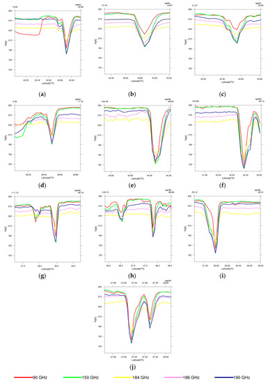
Figure 1.
Brightness temperature distribution along transects crossing the main core of the storm for the analyzed case studies: (a) Bosnia-Herzegovina (2018 UTC); (b) Bulgaria-Sofia (1337 UTC); (c) Bulgaria-Montana (1928 UTC); (d) Germany (1427 UTC); (e) S. Dakota-Vivian (2254 UTC); (f) S. Dakota-Charles (2341 UTC); (g) Colorado-N. Mexico (0337 UTC); (h) Minnesota-N. Dakota (0110 UTC); (i) Argentina-Viale (1239 UTC); (j) Argentina-Liebig (2136 UTC).
As observed by Ferraro et al. [29] and Leppert and Cecil [36], MHS frequencies are very sensitive to the hail bulk and size distribution showing high skills in distinguishing the different concentration of ice into the clouds. Thus, consistent with theory, the magnitude of TB reduction grows with increasing observation frequencies as a function of effective size distribution of ice into the satellite instantaneous field of view (IFOV). Therefore, a high concentration of very large hail strongly depresses TBs at all MHS frequencies revealing not much difference moving from 90 to 157 and 190 GHz. On the contrary, smaller aggregates enhance TBs at the highest frequencies showing low perturbation in the lowest ones.
TBs at all frequencies in Figure 1 decrease when approaching the storm core showing high sensitivity to the hail scattering. The contribution by all channels is well differentiated showing different sounding capabilities with respect to the storm intensity (Figure 1a–d). In particular, the 90 GHz channel exhibits high TB with respect to the ones at 150 and 190 GHz possibly indicating low sensitivity to small hailstones. On the contrary, the same frequency triplet strongly reduces the signal when observing hailstorms over the US Great Plains and AR (Figure 1e–j).
The intense convections over S. Dakota (Vivian and Charles) largely impact on the MHS measurements by reaching very low values when approaching the storm core: TB90min = 114.31 K, TB150min = 107.67 K, TB184min = 124.07 K, TB186min = 114.53 K, and TB190min = 107.78 K. TB minima for the AR hailstorms (Viale and Liebig) are quite low: TB90min < 140 K, TB150min < 130 K, TB184min< 160 K, TB186min < 150 K, TB190min < 130 K. Given the importance of defining the impact of hail on the nominal signal to the satellite and then identify a TB interval where hailstorms can be delineated, on the basis of values listed in Table 1, two classes of hail diameters were considered. For each class the average values of TB minima allow to specify the maximum impact of hail diameters (d) on the MHS frequencies. Results are displayed in Table 2. As expected, large hail is often associated with lower TB values than smaller hail. All channels exhibit high sensitivity to the scattering by hail showing large TB reductions from smaller to larger hail. In particular, hail with d < 10 cm (median value: 4.5 cm) strongly depress the quasi-window channels at 150 and 190 GHz where both signals converge around 175 K. These frequencies reveal a high signal dynamic also by fitting hail d ≥ 10 cm where TBs are 50 K lower than in the previous case. Moreover, by comparing the individual response of these channels, it can be said that the difference (TB150–TB190) oscillates around zero when hail is captured and seems to increase with increasing hail diameter.
Table 2.
Averaged minimum brightness temperature (TB) thresholds at the channel frequencies calculated for the two hail diameter classes. Italics indicate the standard deviation.
The scattering by hail with d ≥ 10 cm strongly affects measurements at 90 GHz where the signal displacement of 70 K specifies the high sensitivity of that frequency to very large hail. This is probably due to the larger wavelength allowing to better identify large particles with respect to higher frequencies that are more sensitive to the smaller aggregates.
The TB differences between the two classes observed at 184 and 186 GHz demonstrate their sensitivity to the presence of hail showing that a change hail size rapidly decreases the TBs. However, since their signal dynamics are closely linked to the water vapor absorption in the middle-upper atmosphere the detection of hail based on these frequencies alone could be problematic with respect to using only window channels.
We can thus state that all MHS frequencies sense the presence of hail, with the physical concept that the sensitivity to the scattering from ice increases with frequency. It needs to be specified that the interaction between hail clouds and the upwelling radiation is complex and strongly non-linear. In fact, the radiation measured by satellite is generally extinguished by a large variety of particles coexisting in the frozen region of the clouds. As demonstrated by several authors [37,38,39,40], the radiation scattered by hail is not unique but associated with other hydrometeors differing in shape, density and size distribution and sometime with the presence of supercooled water above the ice layer, and therefore not easily discriminated from the ice contribution. This justifies the adoption of two wide bins of hail diameters for exploring the TB variations and it can explain the large spread of the data observed in particular in the first bin where the heterogeneity of particle sizes is higher than in the second (the standard deviations decrease correspondingly).
2.1. The MicroWave Cloud Classification (MWCC) Method
To better isolate the hail signature the MicroWave Cloud Classification method (hereafter MWCC) [7,9] was applied. The MWCC originally developed for MHS and now adapted to the ATMS and Special Sensor Microwave Imager/Sounder (SSMIS), exploits the properties of the high frequency channels to classify the cloud type (stratiform/convective) by estimating the cloud top altitude and the phase of hydrometeors. The concept of the MWCC algorithm is based on the probing capability of the MHS channels on the basis of their different weighting function distributions. The MWCC method infers the variation of the nominal signal as observed in clear sky conditions by the spectral channels in the water vapor absorption band at 183.31 GHz. The basic concept is that different stages of cloud formation impacts differently on the channel frequencies at 183.31 GHz. Therefore, the effects of clouds on the MHS water vapor channels can be assessed and capitalized for classifying cloud types according to core-associated scattering.
Figure 2 introduces the conceptual scheme of the MWCC. An idealized convection tower (Figure 2a) progressively grows and impacts on the MHS weighting functions (Figure 2b) as a direct effect of its development phase ([6,41]).
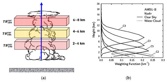
Figure 2.
Conceptual scheme of the MicroWave Cloud Classification (MWCC) algorithm. (a) Artist image describing the impact () of convection development on each water vapor channel as a function of the height of the peak of the weighting functions; (b) channel weighting functions.
Thus, the vertical evolution of convection gradually affects the radiation field around the 183.31 GHz frequencies by “perturbing” their nominal signal at different levels in the atmosphere. Generally, clouds peaking in the low and middle atmosphere affect channels at 190 GHz and 186 GHz. Deep convection strongly scatters the incoming radiation by affecting the highest weighting function of the channel at 184 GHz that peaks around 8 km.
This signal perturbation depends on the channel characteristics, such as the nominal frequency and the weighting functions, and on the cloud structure in terms of its vertical development and microphysical composition. It is computed and compared with the unperturbed radiation field for deriving cloud information. Thus, the vertical evolution of clouds can be derived by evaluating their penetration in the atmosphere on the basis of the signal depression quantified as a percentage variation of the clear sky radiation field (unperturbed background, TBmax).
The MWCC thresholds were statistically calculated from several satellite observations. Radiative transfer simulations were used to support satellite observations in calculating the algorithm offset for reducing the absorption of water vapor which can obscure the signal especially for low level clouds.
The signal variation for each frequency is quantified by the variational normalized index
measuring the absolute value of the net deviation from the unperturbed background radiation and varying between 0 (unperturbed) and 1 (max perturbation).
Hence, all indices are merged in a cascade test which routinely calculates the total perturbation (PMWCC) induced by clouds. The algorithm identifies two main cloud types (stratiform and convective) on the basis of the disturbance due to the penetration of cloud tops into the MHS weighting functions. According to the scattering features observed in the stratiform and convective domain the MWCC method classifies further three sub-classes for each cloud type.
Figure 3 shows the TB150 (<150 K in the core) map of an intense hailstorm over South Dakota (Vivian). The MWCC retrieval scheme identifies a wide region of deep convections (CO1, red), which includes the main core of the hailstorm. In this case, the three water vapor channels measure quite similar TBs because their weighting functions change their typical distribution being flat on the cloud region characterized by large ice.
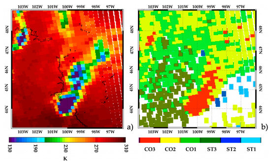
Figure 3.
Hailstorm over South Dakota on 23 July 2010 2254 UTC. (a) Microwave Humidity Sounder (MHS) channel 2 TBs (K); (b) MWCC cloud classification. Colors in b) identify deep (CO3) to shallow (CO1) convection (red to light green) and high (ST3) to low (ST1) stratiform clouds (dark green to cyan).
At the edges of deep convections, the MWCC classifies as moderate (CO2, yellow) and shallow (CO1, light green) convection the rest of the storm. This is due to the temperature weighting functions of the channels at 186 and 190 GHz, which span the middle and lower atmosphere capturing the scattering by smaller frozen hydrometeors near the main core, which increases with frequency.
The TB variation according to the three convective cloud types observed over South Dakota is provided in Figure 4. For shallow and moderate convection (Figure 4a,b) the only TB variations are registered in the channels at 186 and 190 GHz but the perturbation of signal at 184 GHz oscillates in a narrow range since the water vapor absorption generally masks cloud tops below the weighting function distribution. For shallow convections, the signal variation is lower than 15% while for convective clouds in the mid troposphere values go up to 20%.
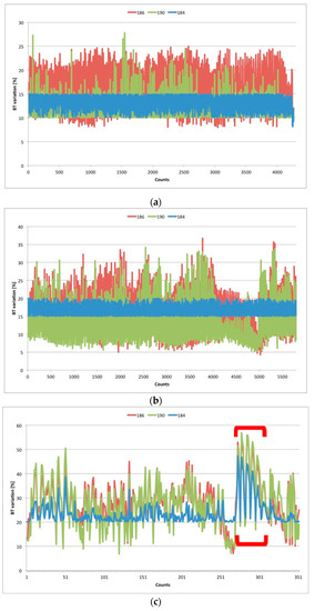
Figure 4.
Distribution of the brightness temperature variations as a function of MWCC convective cloud classification (CO) during the hailstorm over South Dakota, 23 July 2010 2254 UTC. (a) CO1, (b) CO2, and (c) CO3. Red brackets enclose the hail signatures inducing strong TB variations in the three water vapor channels.
During a deep convective event the weighting functions of the three water vapor channels are distorted by the convection tower because the scattering by frozen aggregates perturbs considerably the radiation field. Thus, all frequencies contribute to the identification of cloud features and the MWCC method can help to delimit the cloud areas where the signal is strongly extinguished by hailstones reaching the convective top. From the analysis of the diagram in Figure 4c a region (red brackets) where the signal variations reach a maximum can be seen. This is due to the scattering by large hail which significantly depresses TBs at all frequencies. Therefore, if no-hail is detected, each channel preserves its own dynamics where most prominent oscillations characterize high frequencies (10–50% and 20–40% for and , respectively) and lower values characterize . On the contrary, if hail is detected, the TB depression rapidly increases till 60% at 190 GHz, 53% at 186 GHz, and 48% at 184 GHz. Notably, the scattering by hail is well-distinguished with respect to the whole signal distribution, in particular at (blue lines) where values are generally distributed under the 30% threshold increasing to 50% when hail is observed. This suggests new criteria for isolating hail signatures and calibrate a new method for hail detection. The high potential of the MWCC method in selecting deep convection when coupled with the sensitivity of allow to identify out-of-range signals normally included in the CO3 cloud type. Therefore, by extracting these signals a sub-database for calibrating the hail detection model can be realized. This is the main strategy for powering a probabilistic model used to describe the relationship between the radiometric impact of hail sizes and the net effect of TB reductions.
3. The Hail Detection Model
The physical basis of the hail detection method is based on the relationship between the hail diameters as estimated by hail reports and the scattering signal captured by the MHS channels. Generally, large hail is associated with large TB reduction and the signal extinction increases with frequency (see Table 2). As already noted, the magnitude of the TB reduction is the net volume effect of a number of parameters such as ice in the satellite FOV, its size distribution, and its vertical extent.
In this section, the datasets used to train the model for hail detection are presented. Then the model conceived to calculate the probability of hail occurrences is presented.
3.1. The MWCC Training Dataset
Two independent datasets were used to quantify hail signals and calculate the statistics of the hail detection method. The first, where MHS data are used to directly estimate the impact of hail on TBs, is extracted from the hailstorms listed in Table 1. Each event is binned in the two classes of diameters of Table 2 and then the average TB reduction is calculated.
The second dataset is derived from the 10-year (2000–2009) MHS measurements co-located with hail reports over the US. This matchup dataset already used to develop the prototype algorithm in [29] was derived from satellite overpasses within 5 min and 25 km distance from hailstorm locations, and restricted to an AMSU-B local zenith angle of 25° in order to reduce the impact of changing FOV size due to the scanning geometry.
As discussed in Section 2.1, a preliminary classification of clouds through the MWCC is needed for mapping those convective clouds where hail signature can be recognized. Because the interest is in severe storms, only deep convections classified as CO3 have been isolated and assumed to be associated with hail. Let us consider that in this domain only limited areas of the cloud can be related with hail. Thus, when hail is captured the signal is much higher than that of the background no-hail areas, showing a very strong TB depression.
In order to better discriminate all signals associated with hail, the TB variation at 184 GHz (see Equation (1)) as distributed in the CO3 category has been analyzed. Therefore, three sensitivity classes based on the values have been defined on the basis of the simple concept that tends to increase by increasing the amount of growing ice, which is in turn related to the vertical development of convection. The magnitude of is then related to the convection depth: high values of mean high convection severity (high scattering) and then high probability of hail. Table 3 shows the average TBs for each bin.
Table 3.
Averaged brightness temperatures as function of for different hail diameters (d).
As demonstrated by Cecil [26], the TB magnitude tends to decrease with hail diameter and the impact of hail size is modulated by the observing frequency: high frequencies sense the scattering from a wide range of hail diameters while lower frequencies miss the majority of the scattering signal from smaller ice particles and their use is usually limited to very large hailstones.
Table 3 shows that the average TBs decrease with increasing hail diameters and values. Generally, high values correspond to low TBs reaching the minimum values for d > 10 cm.
A detailed analysis demonstrates that when < 25% the TBs show no noticeable reduction from d lower to higher than 10 cm. However, a comparison between the two first rows of Table 3 highlights that averaged TBs are apparently higher for d > 10 cm with respect to those associated with smaller d. This result appears physically contradictory, but can be justified by considering that in this class the TB variability is due to several factors linked to the intrinsic dynamics of each class. Hailstorms belonging to the class d < 10 cm are generally characterized by a large variety of ice aggregates coexisting on top of convection towers. This large particle size distribution, when segmented by values, tends to fill the first two bins with a tendency to aggregate in the first bin where the median diameter value (4.5 cm) belongs. On the contrary, hailstorms where d > 10 cm are often characterized by hail cores clustered in a restricted area of convective clouds. Then large hail distributes in the bins where > 25% leaving very small frozen hydrometeors (possibly associated with supercooled water) in the first bin where < 25%. The result is that for < 25% the ice scattering mostly impacts on the category d < 10 cm but for bins with > 25% the average TBs largely diverge touching minimum values for d < 10 cm.
The CO3 domain of two hailstorms is segmented in Figure 5 on the basis of values. The first sequence of images (top) refers to the Colorado hailstorm (d < 3.5 cm) and shows the unfiltered patterns of CO3 (5a) and those filtered by 15% < < 25%, 25% < < 35%, and > 35% (Figure 5b,c,d respectively). As seen, only the first two classes capture hail signatures drawing the distribution of main hail cores leading different hail-size diameters. Consistent with the relatively small hail diameters, no hail signals for > 35% have been found.
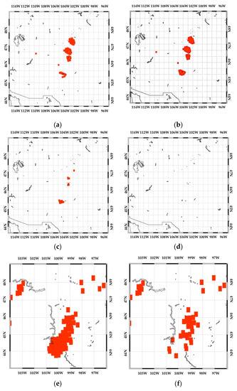
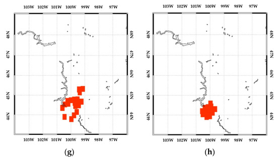
Figure 5.
sensitivity classes applied to the hailstorms over Colorado (a–d) and South Dakota (e,f). The sequencing of CO3 complete domain (a,e) using the thresholds identifies the majority of convective pixels in the class 15%–25% (b,f) while classes with values ranging in 25–35% (c,g) and > 35% (d,h) enclose the main hail cores. Note that no pixels belong to the class > 35% for the Colorado hailstorm where the measured hail diameter at ground was lower than 3.5 cm.
The second series of images displays the event over South Dakota (Vivian) where the measured hail size at the ground was around 11 cm. In this case, the sequencing of the whole dataset (Figure 5e) with the thresholds demonstrate as the smaller ice particles (low scattering) are collected by 15% < < 25%, (Figure 5f) but the signal associated with hail is sampled by classes > 25% (Figure 5g,h). In particular, > 35% (Figure 5h) caught the highest TB reductions correlated to the extinction by very large hail.
The investigation on the individual channels reveals the high capabilities of the MHS frequencies in detecting the variations of cloud ice bulk and estimating the hydrometeor properties during deep convection. Nevertheless, not all channels contribute at the same level of significance. Frequencies at 90, 150, and 190 GHz perform better in describing the ice scattering regime of convective cores containing hail and this makes them primary candidates as proxies for hailstorm detection.
A closer examination of the previous results adds some further considerations. First, low perturbations induced by relatively low scattering as described by < 25% are very difficult to be directly associated with hail signatures. Hence, CO3 cloud features belonging to this class cannot be directly related to hail clouds. Second, moderate to high TB reductions observed for 25% < < 35% can be associated to hail but only the 150 and 190 GHz channels revealed high sensitivity to hail size modifications. This is probably due to the sensitivity of these wavelengths to the minimal variations of ice size distribution while the dynamic range at 90 GHz typically senses scattering by large to very large hail as observed by the > 35% class.
The threshold > 25% is then applied to the whole dataset in order to isolate the TB values useful to calibrate the hail detection model.
In summary, we explore the combinations of the most sensitive MHS channels to evaluate the best frequency differences fitting hail signatures. The TB differences (BTD) between 90, 150, and 190 GHz are displayed in Figure 6. Both combinations including the 90 GHz frequency appear less significant in terms of sensitivity so that they do not recommend themselves for inclusion in the hail detection model. For d < 10 cm the distribution (BT90–BT150) is flat and takes a quadratic shape when d > 10 cm. The difference (BT90–BT190) shows a decreasing exponential distribution when d < 10 cm while the distribution becomes quadratic when d > 10 cm. High sensitivity is demonstrated by the (BT150–BT190) difference exhibiting the same distribution in both hail diameter classes becoming zero for large hail signature as detected by > 35%. The skill of the (BT150–BT190) difference in evidencing hail scattering fits the conceptual model, which is an exponential distribution as a function of hail diameters. Thus, the hail detection model will be trained by exploiting this BTD.
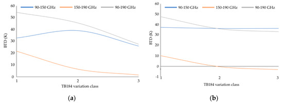
Figure 6.
Brightness temperature differences (BTD) fitting the three classes for hail diameters 2 < d < 10 cm (a) and d > 10 cm (b). Note that the difference (BT150–BT190) shows high sensitivity in capturing hail features with changing diameters.
3.2. AMSU-B Matchup Data
The training data for the hail model stems from a large database of co-located ground hail observations and AMSU-B overpasses. The matchup dataset covers the training period March-September 2000–2009 [29]. Each satellite overpass within 5 min and 25 km distance from the hailstorm location, and restricted to AMSU-B local zenith angle < 25° to avoid low resolution FOVs and reduce the impact of surface type and atmospheric moisture content [42], is retained. The training dataset was investigated by using the thresholds to isolate the TBs correlated with hail signatures. AMSU-B average TBs co-located with surface hail observations are displayed in Table 4.
Table 4.
AMSU-B average TBs by threshold for the training period 2000–2009.
Only data corresponding to > 25% should be considered, where the likelihood of hail signatures is higher. By compacting Table 3 and Table 4, the training dataset of the hail detection model is distributed as in Table 5 by assuming as limits for the TBs the average values of the two tables in the corresponding classes.
Table 5.
Number of training data for the hail detection model.
63.60% (1834) of data populate the class < 35% and 36.40% (1048 data) belong to the class > 35%. Note that the majority of hail sizes shows d < 10 cm with a mode value around 5 cm. Only 324 occurrences (see Table 3) show d > 10 cm with maximum d = 14 cm. Thus, the model is constrained by a statistical population of hail diameters from a few cm or lower to 14 cm within the average TB range in Table 6. Finally, the absolute minimum of the two datasets defines the maximum sensitivity to hail scattering of the 150 and 190 GHz channels involved in the detection algorithm.
Table 6.
Average TBs defining the dynamic range for hail detection.
3.3. The Hail Detection Model
The hail detection model is based on a probability model of growth [43] that exploits the TBs at 150 and 190 GHz. The general concept is based on the inverse proportionality between the upwelling radiation and hail cross-sections. As demonstrated above, the frequencies at 150 and 190 GHz are the most sensitive to the presence of hail being subject to a modification of their radiation field as a function of hail diameter. Furthermore, although their dynamics is pretty similar, the signal at 150 GHz channel tends to decrease more steeply than at 190 GHz. Therefore, we assume as model for hail detection a modified sigmoidal function as follows:
where x and y are the TBs at 150 and 190 GHz, respectively. The difference between these two frequencies is demonstrated to be very sensitive to the growth of ice aggregates particularly when hail size is the order of centimeters. Eq. 2 shows boundaries between 0 with clear sky conditions and 0.99 when hail is observed.
The probability model described by Equation (2) was trained with the entire dataset described in Table 5 knowing that signatures from very large hail, typically correlated with >8–10 cm, can be found when >35%.
Equation (2) is also reinforced by a variable inspired by the concept of carrying capacity [44] of biological species, that is the maximum population size that the environment can sustain indefinitely or on the contrary the maximal load of the environment which modulates the population equilibrium. The carrying capacity is then a sort of regulator of population dynamics typically approximated by a probability model, which controls the occurrence of an overshooting of survival conditions that in long term leads to the collapse of the species. In the case of hail detection, the population (hail) impacts on the upwelling radiation (environment) by increasing the scattering effects (environment sustainability). The growth of hail sizes increases the scattering effects and then decreases the radiation to the satellite.
This process is well described by Equation (2), which approximates the expected probability distribution as a function of decreasing TBs. To govern the dynamics of the probability model by stopping the computation when the sensitivity reaches its maximum (overshooting) and no hail signatures can be recognized (saturation condition), a dynamic carrying capacity was introduced. The carrying capacity attains values in the range [0,1] and is described by the dimensionless variable K,
where α = 104 K and x is the TB at 150 GHz, frequency chosen because it reaches saturation conditions faster. For K << 1 the population load is minimum while for K = 1 the model reaches the overshooting and the computation stops. A realistic distribution of Equations (2) and (3) fed by data in Table 6 is reported in Figure 7. Note that both distributions converge to 1 when the minimum value is reached but largely diverge for the maximum TB.
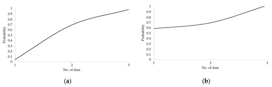
Figure 7.
Distribution of probability model (Equation (2)) when applied to data in Table 6. The model realistically approximates the probability distribution (a) and the carrying capacity (b) when the model runs with the whole dataset.
Therefore, by regressing Equations (2) and (3) we derive a compact general model able to represent the hail size distribution as a function of TB depression. The result is a new function H(K) that maps the probability of hail detection as only function of TB150.
The dynamics of the hail detection model when applied to the whole dataset (2882 data) is reported in Figure 8a. The distribution of probability starts with a carrying capacity about 0.40, which roughly corresponds to TB150 > 270 K and is quite far from hail signatures as found in Table 6. Thus, for finding a numerical value that fits the hail signal, Equation (4) is adjusted on the basis of TB150 values displayed in Table 6 used as input to Figure 8b. The hail detector starts with probability values > 0. 36 (TB150 = 181.30 K) generally associated with graupels or small hail aggregates to large hail (2 < d < 10 cm) then reaches values around 0.53 when TB150 = 152.51 K, which is associated to the transition between large hail (d < 10 cm) to super hail (d > 10 cm) and finally the model stops (saturation condition) when TB150 approaches the critical value 103.70 K, i.e., the absolute minimum found in the training dataset.
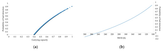
Figure 8.
Distribution of hail probabilities calculated from eq. 4 when applied to the whole dataset (a) and the hail model as a function of TB150 (b).
It is then clear the advantage of using a compact formula (Equation. (4)) in approximating such a complex interaction mechanism between hail and radiation field which typically is no-linear. As a final comment, ought to be said that since the model has been developed and tested during the “warm” months when hail typically forms (Mar-Sep) such possible spurious effects can be arisen over from frozen soils. Experimental applications demonstrate very few false alarms when the hail detector is integrated into the MWCC computational scheme which is able to screen out the surface effects.
4. Validation
To validate the performances of the hail detection model described by eq. 4 (hereafter MWCC-Hail) twelve years of mean AMSU-derived hail occurrences have been used. Each MHS overpass was combined with hail occurrences at the ground within 1° grid box lat/lon and represents the total number of hailstorms over the entire spatial domain. The analysis is based on 12-year data March through September, i.e., the period of peak hailstorm occurrence.
The MWCC-Hail is applied to all available MHS data for the whole period, not just to those co-located with the storm reports, which represent a very small subsample of all possible satellite measurements. Thus, the MWCC-Hail model-derived hail will cover different time and space domains with respect to those we observe from the ground.
An inspection of the plates (a) and (b) in Figure 9 demonstrates the similarities between the MWCC-Hail and the SPC storm reports. The majority of hail occurrences are located in the Central US with a clear coverage of the Eastern US. Even though the MWCC-Hail tends to underestimate the number of events with a maximum number of occurrences around 40 with respect to more than 60 as reported by the storm reports, the area of maxima is well reproduced.
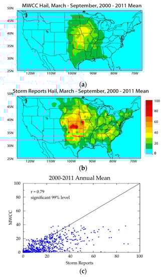
Figure 9.
2000–2011 annual mean distribution of hail events from the (a) the MWCC hail detection model and (b) surface storm reports; (c) scatter plot of the correlation between the two datasets.
The overall performance of MWCC-Hail quantified in the scatterplot of Figure 9c confirms on one hand the underestimation with respect to hail reports while at the same time the high correlation coefficient (0.79) indicates notable retrieval capabilities.
The seasonal distribution of the number of events and their location from MWCC-Hail and SPC storm reports are displayed in Figure 10. Although the hail occurrences are generally underestimated, MWCC-Hail shows high sensitivity in identifying the location of maxima and their areal extent fitting the seasonality of the events. In fact, the peak in May-June is detected as well as the minimum in August-September. Note that the missing retrievals on the Eastern CONUS in May-June are associated with hail events characterized by small hail diameters (5196 data with 2.2 cm and 1418 with 4.1 cm) often corresponding to probability values under the minimum threshold (0.36). However, the statistical comparison (Figure 11) shows a good agreement between retrieved and observed data with correlation values ranging between 0.60 in September and 0.75 in May.
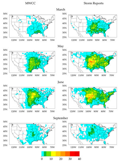
Figure 10.
Twelve-year (2000–2011) mean number of hail events over CONUS for the months of March, May, June and September from MWCC-Hail retrievals (left) and official storm reports (right).
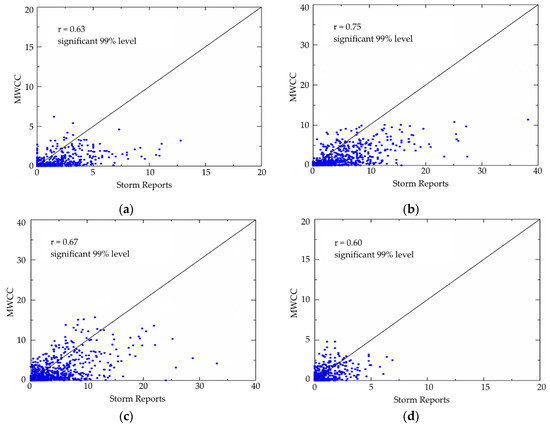
Figure 11.
(a) March, (b) May, (c) June and (d) September scatter plots for the mean 2000–2011 maps of Figure 10.
As an overall consideration on the validation results, note that while the model MWCC-Hail shows high capability in detecting hail events and their areal distribution it performs worse when small or very small hail diameters dominate the observed hailstorm. Additionally, potential overestimates can be registered during the winter season when the background conditions, often controlled by frozen soils, may affect the retrievals. This issue deserves further studies.
Finally, the intrinsic flexibility of the probability-based approach reinforces the potential of MWCC-Hail both in identifying a variety of hail size distributions and fit similar PMW frequencies from other satellite instruments, as demonstrated in Section 5.
5. Application Examples
The performances of MWCC-Hail will be displayed by applying the model to several hailstorms characterized by different regime of severity. The aim of this section is showing the sensitivity of the detector to different hail conditions by prospecting its employing in reconstructing the hail patterns on the global scale. Accordingly, probability values lower than 0.36 are classified as no hail, values in the range 0.36–0.60 are associated to hail, and probabilities greater than 0.60 are associated to the super hail category.
Thus, we propose a series of examples where the MWCC-Hail will be experimentally applied to all MHS-like radiometers currently flying on the GPM constellation. Although the well-known technical differences between the MHS-like radiometers and MHS (reference instrument) the present outcomes demonstrate the high skills of model in identifying hail clouds and discern hail size on the basis of likelihood values. These results have then stimulated new studies where the hail detection model described by Equation (4) will be recalibrated to fit better the instrumental characteristic of the MHS-like radiometers by improving the current retrievals.
Figure 12 shows some of the hail events reported in Table 1. In all plates it can be seen the capability of model to identify the convective cores where the presence of hail is detected. All of these events were characterized by a hail-train clusters where the diameters significantly change.
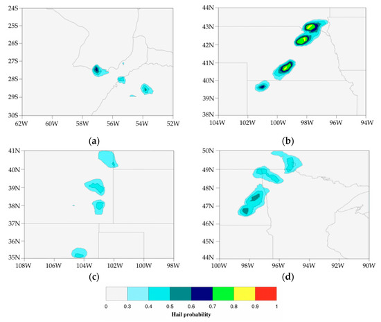
Figure 12.
Hail probability as calculated by the MWCC-Hail for hailstorms over (a) Argentina (Colonia) 13 Nov 2017 2136 UTC, (b) South Dakota (Charles) 21 Aug 2007 2341 UTC, (c) Colorado–New Mexico 9 May 2017 0337 UTC, and (d) Minnesota–North Dakota 10 Jun 2017 0237 UTC.
The retrievals show that the highest severity is registered over South Dakota where hail probability reaches 0.80 (super hail) in the smaller cores and 0.70 in the surroundings. The other cases can be classified from moderate to severe hailstorms due to the high values of hail probability reaching the maximum of 0.70 over Argentina and the lowest values (0.40–0.50) retrieved over Colorado–New Mexico. Noteworthy the event over Minnesota–North Dakota exhibiting two different hail regimes: probability values 0.50–0.60 over North Dakota typically associated to large hail and values around 0.40 over Minnesota which delineate smaller hail diameters.
Figure 13 documents the first experiment where the MWCC-Hail is applied to the GPM constellation. Since not all satellites covers the same event we evaluate the performances of detection by using two separate hailstorms. Applying the MWCC-Hail to the GMI data on the heavy hailstorm over Naples on 5 September 2015 (Figure 13a) we can note as the severity of the event is fully captured by the model which identifies the intensity of each hail cluster. The borders of system are flagged by hail probability close to 0.50 while the main core of deep convection reaches values over than 0.90 which is associated to super hail as well documented by surface hail reports.
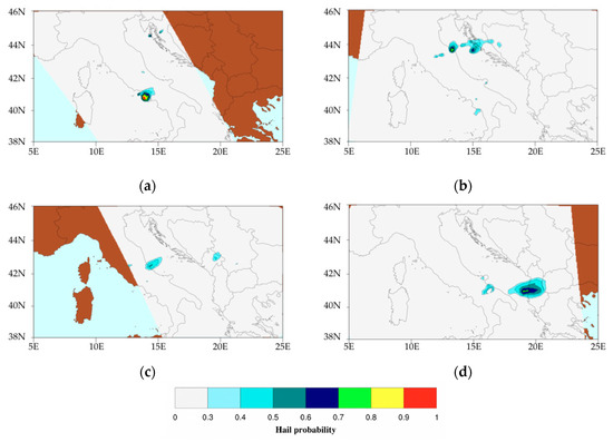
Figure 13.
MWCC-Hail applied to the GPM constellation during two severe hailstorms. The hail probability is calculated during heavy hailstorms with (a) GMI frequencies on 5 September 2015 over Naples, and on 10 Jul 2019 over the Adriatic Sea coast with (b) F17-SSMIS, (c) N20-ATMS, and (d) N19-MHS, respectively.
On 10 July 2019 the Adriatic coast of Italy was hit by a long sequence of severe storms triggered from the early morning in the North-East part of Italy and dissolved during the night over Greece. The series of deep convections rapidly evolved in severe hailstorms is well-reconstructed by the MWCC-Hail when applied to MHS-like radiometers of the GPM constellation. The SSMIS caught the very large hail hitting the city of Milano Marittima (Figure 13b, hail probability: 0.80) while the ATMS identified the hail cloud over the city of Pescara (Figure 13c, hail probability: 0.60), and finally the MHS, used as a reference target, spotted the system traveling from Italy to Greece detecting a super hail cloud over Albania (Figure 13d).
6. Summary and Conclusions
A new model for hail detection based on satellite PMW radiometers has been presented. By using the MicroWave Cloud Classification (MWCC) method only deep convective clouds were selected to isolate hail signatures. In order to reproduce the signal attenuation due to hail scattering a probabilistic method was adopted for describing the TB reductions as a function of hail diameters. The carrying capacity concept was used to force the convergence of the model when saturation conditions are reached. The result is a simple one-variable (TB150) equation that calculates the probability associated with the presence of hail by identifying large and very large hail signatures. The validation with 12-year matchup data demonstrates the high performance of the model in detecting hail by showing strong correlation with validating dataset and reproducing well the seasonality of hailstorms over CONUS.
The MWCC-Hail model is now applied in investigating the presence of hail patterns during deep convection over mid-latitude and tropical regions where the majority of heavy rainstorms are typically due to the melting of large ice hydrometeors (graupel and hail) before reaching the ground. The investigation of hail amounts in convective rain both in terms of size and occurrences is instrumental to a better understanding of the impact of frozen hydrometeors in inducing extreme rainfalls in view of confirming the hypothesis of severe storms increase due to climate change. In this perspective, the MWCC-Hail model has been integrated in the computational scheme of the water vapor strong lines at 183 GHz (183-WSL) algorithm [4] to associate hail probability with precipitation retrievals so that the incidence of hail in the formation of heavy rain can be evaluated.
The flexibility of the hail detection model MWCC-Hail stimulated further applications to the GPM constellation, where MHS-like radiometers currently orbit, showing very high performances in detecting hail patterns. The first results presented here have motivated a new sensitivity analysis to evaluate the generalization of the model to the new radiometers by assessing the impact of MHS-like frequencies of PMW radiometers orbiting of the GPM constellation (ATMS ch17: 165.5 GHz; GMI ch11: 166.5 GHz). This opens the way to the applicability of the MWCC-Hail at the global scale for building a satellite-based worldwide hail climatology.
We conclude that the potential offered by the hail detection model discussed in this work in terms of its generalization to all MHS-like radiometers encourages further studies of a geostationary high-frequency PMW sensor. Such instrument is under discussion since almost 20 years within the international satellite community. This challenging mission will definitely change the current prospective of the atmospheric studies introducing the possibility to continuously observe meteorological phenomena impacting the hydrologic cycle.
Author Contributions
S.L. conceived the method and carried out the data analysis. V.L. contributed to the concept. R.R.F. and J.B. contributed to the validation. All authors contributed to the writing. All authors have read and agreed to the published version of the manuscript.
Funding
This research received no external funding.
Acknowledgments
This work is performed in the context of the scientific cooperation defined by the MOU between the Institute of Atmospheric Sciences and Climate of the Italian National Research Council (CNR-ISAC) and the National Oceanic and Atmospheric Administration (NOAA). Giulio Monte is gratefully acknowledged for drawing Figure 1, Figure 12 and Figure 13.
Conflicts of Interest
The authors declare no conflict of interest.
Abbreviations
| AMSU-B | Advanced Microwave Sounding Unit-B |
| AR | Argentina |
| ATMS | Advanced Technology Microwave Sounder |
| BTD | Brightness Temperature Difference |
| CONUS | Conterminous United States |
| DPR | Dual-frequency Precipitation Radar |
| ESSL | European Severe Storms Laboratory |
| EU | Europe |
| FOV | Field of View |
| IFOV | Instantaneous FOV |
| IR | InfraRed |
| GMI | GPM Microwave Imager |
| GPM | Global Precipitation Measurement mission |
| MHS | Microwave Humidity Sounder |
| MWCC | MicroWave Cloud Classification method |
| NOAA | National Oceanic and Atmospheric Administration |
| PMW | Passive Microwave |
| PMWCC | Perturbation of MWCC |
| SPC | Storm Prediction Center |
| SSM/I | Special Sensor Microwave/Imager |
| SSMIS | Special Sensor Microwave Imager/Sounder |
| TB | Brightness Temperature |
| TRMM | Tropical Rainfall Measuring Mission |
| US | United States of America |
| VIS | Visible |
| 183-WSL | Water vapor Strong Lines at 183 GHz algorithm |
References
- Ferraro, R.R.; Weng, F.; Grody, N.; Zhao, L.; Meng, H.; Kongoli, C.; Pellegrino, P.; Qiu, S.; Dean, C. NOAA operational hydrological products derived from the advanced atmospheric sounding unit. IEEE Trans. Geosci. Remote Sens. 2005, 43, 1036–1049. [Google Scholar] [CrossRef]
- Staelin, D.H.; Chen, F.W. Precipitation observations near 54 and 183 GHz using the NOAA-15 satellite. IEEE Trans. Geosci. Remote Sens. 2000, 38, 2322–2332. [Google Scholar] [CrossRef]
- Sanò, P.; Panegrossi, G.; Casella, D.; Marra, A.C.; D’Adderio, L.P.; Rysman, J.F.; Dietrich, S. The passive microwave neural network precipitation retrieval (PNPR) algorithm for the CONICAL scanning Global Microwave Imager (GMI) radiometer. Remote Sens. 2018, 10, 1122. [Google Scholar] [CrossRef]
- Laviola, S.; Levizzani, V. The 183-WSL fast rainrate retrieval algorithm. Part I: Retrieval design. Atmos. Res. 2011, 99, 443–461. [Google Scholar] [CrossRef]
- Laviola, S.; Levizzani, V.; Cattani, E.; Kidd, C. The 183-WSL fast rainrate retrieval algorithm. Part II: Validation using ground radar measurements. Atmos. Res. 2013, 134, 77–86. [Google Scholar] [CrossRef]
- Hong, G.; Heygster, G. Detection of deep convective clouds from AMSU-B water vapor channels measurements. J. Geophys. Res. 2005, 110, D05205. [Google Scholar] [CrossRef]
- Laviola, S.; Levizzani, V. Observing precipitation by means of water vapor absorption lines: A first check of the retrieval capabilities of the 183-WSL rain retrieval method. Ital. J. Remote Sens. 2009, 41, 39–49. [Google Scholar] [CrossRef]
- Funatsu, B.M.; Claud, C.; Chaboureau, J.-P. Potential of Advanced Microwave Sounding Unit to identify precipitating systems and associated upper-level features in the Mediterranean region: Case studies. J. Geophys. Res. 2007, 112, D17113. [Google Scholar] [CrossRef]
- Levizzani, V.; Laviola, S.; Cattani, E.; Costa, M.J. Extreme precipitation on the Island of Madeira on 20 February 2010 as seen by satellite passive microwave sounders. Eur. J. Remote Sens. 2013, 46, 475–489. [Google Scholar] [CrossRef]
- Bauer-Messmer, B.; Waldvogel, A. Satellite data detection and prediction of hail. Atmos. Res. 1997, 43, 217–231. [Google Scholar] [CrossRef]
- De Coning, E.; Gijben, M.; Maseko, B.; van Hemert, L. Using satellite data to identify and track intense thunderstorms in South and southern Africa. S. Afr. J. Sci. 2015, 111, 2014-0402. [Google Scholar] [CrossRef]
- Rosenfeld, D.; Woodley, W.L.; Lerner, A.; Kelman, G.; Lindsey, D.T. Satellite detection of severe convective storms by their retrieved vertical profiles of cloud particle effective radius and thermodynamic phase. J. Geophys. Res. 2008, 113, D04208. [Google Scholar] [CrossRef]
- Mecikalski, J.R.; Watts, P.D.; Koenig, M. Use of Meteosat Second Generation optimal cloud analysis fields for understanding physical attributes of growing cumulus clouds. Atmos. Res. 2011, 102, 175–190. [Google Scholar] [CrossRef]
- Merino, A.; López, L.; Sánchez, J.L.; García-Ortega, E.; Cattani, E.; Levizzani, V. Daytime identification of summer hailstorm cells from MSG data. Nat. Hazards Earth Syst. Sci. 2014, 14, 1017–1033. [Google Scholar] [CrossRef]
- Sánchez, J.L.; Gil-Robles, B.; Dessens, J.; Martin, E.; López, L.; Marcos, J.L.; Berthet, C.; Fernández, J.T.; García-Ortega, E. Characterization of hailstone size spectra in hailpad networks in France, Spain, and Argentina. Atmos. Res. 2009, 93, 641–654. [Google Scholar] [CrossRef]
- Prein, A.; Holland, G.J. Global estimates of damaging hail hazard. Weather Clim. Extrem. 2018, 22, 10–23. [Google Scholar] [CrossRef]
- Cintineo, J.L.; Smith, T.M.; Lakshmanan, V.; Brooks, H.E.; Ortega, K.L. An objective high-resolution hail climatology of the contiguous United States. Weather Forecast. 2012, 27, 1235–1248. [Google Scholar] [CrossRef]
- Nisi, L.; Martius, O.; Kunz, M.; Germann, U. Spatial and temporal distribution of hailstorms in the Alpine region: A long-term, high resolution, radar-based analysis. Quart. J. R. Meteorol. Soc. 2016, 142, 1590–1604. [Google Scholar] [CrossRef]
- Smith, T.M.; Lakshmanan, V.; Stumpf, G.J.; Ortega, K.L.; Hondl, K.; Cooper, K.; Calhoun, K.M.; Kingfield, D.M.; Manross, K.L.; Toomey, R.; et al. Multi-Radar Multi-Sensor severe weather and aviation products: Initial operating capabilities. Bull. Am. Meteorol. Soc. 2016, 97, 1617–1630. [Google Scholar] [CrossRef]
- Punge, H.J.; Bedka, K.M.; Kunz, M.; Werner, A. A new physically based stochastic event catalog for hail in Europe. Nat. Hazards 2014, 73, 1625–1645. [Google Scholar] [CrossRef]
- Warren, R.A.; Ramsay, H.A.; Siems, S.T.; Manton, M.J.; Peter, J.R.; Protat, A.; Pillalamarri, A. Radar-based climatology of damaging hailstorms in Brisbane and Sydney, Australia. Quart. J. R. Meteorol. Soc. 2019. [Google Scholar] [CrossRef]
- Ajvazyan, H.M.; Ajvazyan, H.H. Hail embryons detection in clouds using passive and active radars in millimeter and submillimeter wave bands. Int. J. Infrared Millim. Waves 1993, 14, 1155–1174. [Google Scholar] [CrossRef]
- Spencer, R.W.; Olson, W.S.; Rongzhang, W.; Martin, D.W.; Weinman, J.A.; Santek, D.A. Heavy thunderstorms observed over land by the Nimbus-7 scanning multichannel microwave radiometer. J. Clim. Appl. Meteorol. 1983, 22, 1041–1046. [Google Scholar] [CrossRef]
- Spencer, R.W.; Howland, M.R.; Santek, D.A. Severe storm identification with satellite microwave radiometry: An initial investigation with Nimbus-7 SMMR data. J. Clim. Appl. Meteorol. 1987, 26, 749–754. [Google Scholar] [CrossRef]
- Spencer, R.W.; Santek, D.A. Measuring the global distribution of intense convection over land with passive microwave radiometry. J. Clim. Appl. Meteorol. 1985, 24, 860–864. [Google Scholar] [CrossRef][Green Version]
- Cecil, D.J. Passive microwave brightness temperatures as proxies for hailstorms. J. Appl. Meteorol. Climatol. 2009, 48, 1281–1286. [Google Scholar] [CrossRef]
- Cecil, D.J. Relating passive 37-GHz scattering to radar profiles in strong convection. J. Appl. Meteorol. Climatol. 2011, 50, 233–240. [Google Scholar] [CrossRef]
- Cecil, D.J.; Blankenship, C.B. Toward a global climatology of severe hailstorms as estimated by satellite passive microwave imagers. J. Clim. 2012, 25, 687–703. [Google Scholar] [CrossRef]
- Ferraro, R.R.; Beauchamp, J.; Cecil, D.J.; Heymsfield, G. A prototype hail detection algorithm and climatology developed with the Advanced Microwave Sounding Unit (AMSU). Atmos. Res. 2015, 163, 24–35. [Google Scholar] [CrossRef]
- Ni, X.; Liu, C.; Zhang, Q.; Cecil, D.J. Properties of hail storms over China and the United States from the Tropical Rainfall Measuring Mission. J. Geophys. Res. 2016, 121, 12031–12044. [Google Scholar] [CrossRef]
- Ni, X.; Liu, C.; Cecil, D.J.; Zhang, Q. On the detection of hail using satellite microwave radiometers and precipitation radar. J. Appl. Meteorol. Climatol. 2017, 56, 2693–2709. [Google Scholar] [CrossRef]
- Marra, A.C.; Porcù, F.; Baldini, L.; Petracca, M.; Casella, D.; Dietrich, S.; Mugnai, A.; Sanò, P.; Vulpiani, G.; Panegrossi, G. Observational analysis of an exceptionally intense hailstorm over the Mediterranean area: Role of the GPM Core Observatory. Atmos. Res. 2017, 192, 72–90. [Google Scholar] [CrossRef]
- Mroz, K.; Battaglia, A.; Lang, T.J.; Cecil, D.J.; Tanelli, S.; Tridon, F. Hail-detection algorithm for the GPM Core Observatory satellite sensors. J. Appl. Meteorol. Climatol. 2017, 56, 1939–1957. [Google Scholar] [CrossRef]
- Mroz, K.; Battaglia, A.; Lang, T.J.; Tanelli, S.; Sacco, G.F. Global Precipitation Measuring Dual-Frequency Precipitation Radar observations of hailstorm vertical structure: Current capabilities and drawbacks. J. Appl. Meteorol. Climatol. 2018, 57, 2161–2178. [Google Scholar] [CrossRef]
- Bang, S.D.; Cecil, D.J. Constructing a multifrequency passive microwave hail retrieval and climatology in the GPM domain. J. Appl. Meteorol. Climatol. 2019, 58, 1889–1904. [Google Scholar] [CrossRef]
- Leppert, K.D., II; Cecil, D.J. Signatures of hydrometeor species from airborne passive microwave data for frequencies 10-183 GHz. J. Appl. Meteorol. Climatol. 2015, 54, 1313–1334. [Google Scholar] [CrossRef]
- Bauer, P.; Moreau, E.; Di Michele, S. Hydrometeor retrieval accuracy using microwave window and sounding channel observations. J. Appl. Meteorol. 2005, 44, 1016–1032. [Google Scholar] [CrossRef]
- Bennartz, R.; Bauer, P. Sensitivity of microwave radiances at 85–183 GHz to precipitating ice particles. Radio Sci. 2003, 38, 8075. [Google Scholar] [CrossRef]
- Skofronick-Jackson, G.M.; Gasiewski, A.J.; Wang, J.R. Influence of microphysical cloud parameterizations on microwave brightness temperatures. IEEE Trans. Geosci. Remote Sens. 2002, 40, 187–196. [Google Scholar] [CrossRef]
- Hong, G.; Heygster, G. Sensitivity of microwave brightness temperatures to hydrometeors in a tropical deep convective cloud system at 89–190 GHz. Radio Sci. 2005, 40, RS4003. [Google Scholar] [CrossRef]
- Wang, J.R.; Zhan, J.; Racette, P. Storm-associated microwave radiometric signatures in the frequency range of 90–220 GHz. J. Atmos. Ocean. Technol. 1997, 14, 13–31. [Google Scholar] [CrossRef]
- Karbou, F.; Prigent, C.; Eymard, L.; Pardo, J. Microwave land emissivity calculations using AMSU measurements. IEEE Trans. Geosci. Remote Sens. 2005, 43, 948–958. [Google Scholar] [CrossRef]
- Verhulst, P.-F. Recherches mathématiques sur la loi d’accroissement de la population. Nouv. Mémoires l’Académie R. Sci. Belles-Lett. Brux. 1845, 18, 14–54. Available online: http://eudml.org/doc/182533 (accessed on 12 February 2020).
- Mayer, P.S.; Ausbel, J.H. Carrying capacity: A model with logistically varying limits. Technol. Forecast. Soc. Chang. 1999, 61, 209–214. [Google Scholar] [CrossRef]


© 2020 by the authors. Licensee MDPI, Basel, Switzerland. This article is an open access article distributed under the terms and conditions of the Creative Commons Attribution (CC BY) license (http://creativecommons.org/licenses/by/4.0/).