1. Introduction
With the development of laser scanning and image stereo matching, 3D point clouds have emerged in large numbers and become an important type of geometric data structure [
1]. Efficient and effective semantic feature learning for 3D point clouds has been an urgent problem for further analysis tasks such as classification and segmentation, which have enormous real-world applications such as autonomous driving, 3D reconstruction, and digital cities [
2,
3].
Recently, benefiting from the powerful feature learning capability of deep learning networks [
4,
5,
6], researchers have attempted to generalize deep learning from regular grid domains (e.g., images, speeches) to irregular 3D point clouds [
7,
8,
9,
10]. However, because of the irregular data structure of 3D point clouds, standard convolutional neural networks (CNNs) cannot be directly applied to them. To address this problem, the most intuitive way is to divide the 3D point cloud space into regular 3D voxels [
11,
12,
13,
14] or project the 3D point cloud onto 2D images from multiple views [
15,
16,
17,
18], so that the CNNs can be applied directly. However, since the 3D point clouds only record the surface points of 3D objects, the 3D volumetric representation inevitably leads to computation consumption and resolution limitation, while the multi-view projection is sensitive to the mutual occlusion among objects [
7]. More recently, PointNet [
1] introduced a set-based point cloud deep learning network, which allows researchers to directly extract the discriminative features of point clouds by using simple multilayer perceptron (MLP) and a global aggregation function (e.g., the max function). However, the set-based method neglects the spatial neighboring relation between points, which contains fine-grained geometric structures for 3D point cloud analysis.
In fact, the convolution, which is the core of CNNs, can be seen as a template-matching process between the input signal and the convolution kernels. Each convolution kernel has its specific function and is activated when it meets the corresponding structure (e.g., the edge of the image). Inspired by this, the key of our structure-aware convolution (SAC) is to extract the local geometric structure of point clouds by matching each point’s neighborhoods with a series of 3D kernels with specific structures (as shown in
Figure 1). Similarly, the interested geometric structures in 3D point clouds is activated when they are matched with our kernels. To adapt to the complex real situations, the geometric structure of the 3D kernels is adaptively learned from the training dataset.
Specifically, for each point in the point cloud, we first find its neighborhoods as a point set and then match it with the kernel which also consists of a set of learnable 3D points. During the training phase, the kernels are guided to approximate the geometric structures that exist in the training data. However, different from regular 2D images, in which the coordinates of each neighboring pixel are fixed and the geometric structures are reflected by changing gray values, our kernels for 3D point clouds need to be matched with the coordinates of the neighboring points. When the kernels are well trained, they form a series of 3D geometric structures that can be used to capture the corresponding structures in the point clouds.
Our SAC focuses on capturing the local geometric structures of 3D point clouds; it is a simple yet efficient module that can be embedded into other existing point cloud deep learning networks such as PointNet [
1], PointNet++ [
19], and KCNet [
20]. To verify the effectiveness of our proposed SAC, we experimentally applied it to various point cloud analysis tasks, including object classification and semantic segmentation, on three public datasets. Experimental results show that the proposed SAC is efficient to capture the geometric structures of the 3D point clouds and efficiently improves the performance of the recently developed point cloud deep learning networks.
Overall, the main contributions of this paper can be summarized as follows:
We propose a novel structure-aware convolution (SAC) to explicitly capture the geometric structure of point clouds by matching each point’s neighborhoods with a series of learnable 3D point kernels (which can be regarded as 3D geometric “templates”);
We show how to integrate our SAC into existing point cloud deep learning networks, and train end-to-end point cloud classification and segmentation networks;
We experimentally demonstrate the effectiveness of our SAC by improving the performance of the recently developed point cloud deep learning networks (PointNet [
1], PointNet++ [
19], and KCNet [
20]) on both classification and segmentation tasks.
3. Methods
We propose a novel structure-aware convolution for geometric structure learning on point clouds with a series of learnable 3D kernels (
Section 3.1), and show its relation with standard convolution on a regular 2D grid (
Section 3.2). Afterward, we show how to integrate the proposed SAC into recently developed deep learning networks for both point cloud classification and segmentation (
Section 3.3).
3.1. Structure-Aware Convolution
We denote the given point cloud as , where represents the coordinates of the -th point. represents the set of neighboring points of (including itself), and our goal is to recognize the geometric structure that is formed by the neighboring points. For example, is it a plane, a spherical surface, a corner, or another geometric structure?
To this end, our SAC is designed to describe these geometric structures with a series of 3D kernels, where each kernel consists of a set of learnable 3D points. When the geometric structure formed by the kernel is well matched with the one formed by the neighboring points (e.g., a plane), then the current point is correspondingly activated.
Specifically, we denote each 3D kernel as
(
), which is a set of 3D points with learnable coordinates, and
is the number of kernels. The corresponding output of the SAC can be formulated as follows:
where
is the number of neighboring points and
is a constant parameter.
is the one-to-one mapping function between sets of neighboring points and kernel points, so that the distance between the two sets is minimized, which corresponds to the maximum output of
.
Consequently, the extracted geometric structure can be expressed as an -dimensional feature vector . Each kernel represents a specific geometric structure and an attempt is made to match the neighboring points. If they can be perfectly matched, the corresponding channel is activated as a value close to 1, and the other channel is close to 0.
At the beginning of the training phase, the initial kernel points are uniformly scattered in a sphere, which means no meaningful geometric structures are formed by the convolution kernels and they cannot be used to match any geometric structures. During the training process, each convolution kernel is guided to approximate a specific geometric structure contained in the training data (an illustration of the training process of our SAC kernel is shown in
Figure 2). Thus, our learned SAC kernels can be matched with and represent kinds of complex geometric structures that exist in real situations during the testing phase.
3.2. Relationship to Standard Convolution
3.2.1. Reformulation of Standard Convolution
We first revisit the standard convolution on regular 2D images (
Figure 3). For each pixel of the regular image, we first need to find its neighboring pixels in a convolution window as a matrix
I (here the image with a single channel is considered for convenience). We denote the convolution kernel as
W, which is also a 2D matrix. Then, the convolution on the regular 2D image can be expressed as follows:
where
represents the output of the convolution,
represents the index of the pixel in the neighbor patch or convolution kernel, and
is the corresponding bias.
More generally, if we flatten the matrix
I and convolution kernel
W to a one-dimensional vector with the same order, the above convolution on the regular image can reformulated as follows:
where
is a function about the convolution kernel and the neighboring pixels. We can see that the convolution on the 2D image is actually a process of weighted summation of the neighboring pixels, where the values of the convolution kernel are the corresponding weights.
3.2.2. Reformulation of SAC
Similar to 2D images, our SAC also aims to aggregate the information in its neighboring region for each point, as shown in Equation (1). Suppose
is the optimization mapping function between the sets of neighboring points and kernel points in Equation (1). In practice, since
, the first-order Taylor expansion of the right side of Equation (1) is already a good approximation to
. Therefore, we have the following:
where
and
are the parameters related to
. Compared to the standard convolution in Equation (3), our SAC can actually be simplified as a similar formulation (Equation (4)) but with a modified convolution kernel function
.
However, unlike 2D images with regular data structure and their neighbors leveraging the natural fixed relative positions, the neighboring points of 3D point clouds can appear in any position of the 3D space and have no certain order. To handle this problem, a mapping function
that matches each neighboring point to its corresponding kernel point is needed, so that the kernel points can be applied to their corresponding neighboring points. Specifically, for each neighboring point
, we should first find its corresponding kernel point
, and the distance is then calculated between the corresponding point pair in the kernel and neighbor sets (as shown in
Figure 3).
3.3. Deep Learning Networks with the Proposed SAC
According to the above analysis, our SAC actually provides a flexible geometric structure extractor which can be easily embedded into existing point cloud deep learning networks. In this section, we show how to construct the corresponding deep learning networks with our proposed SAC.
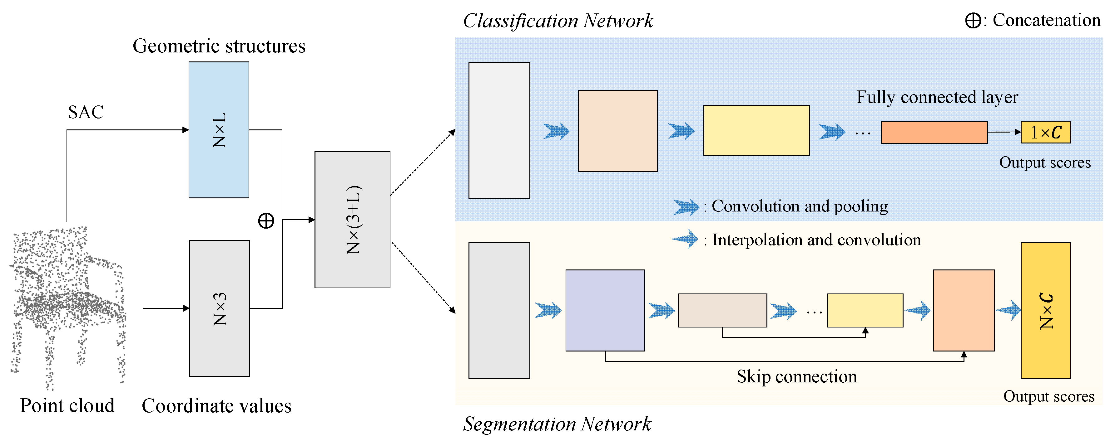
Specifically, the architecture of the classification and segmentation networks with our SAC is illustrated in
Figure 4. For each point
, we first find its neighboring points
according to their spatial distance, and then match them with a series of 3D kernels
. Therefore, the output of our SAC is an
-dimensional feature vector
, where each
can be regarded as the matching degree between neighboring points and the
-th convolution kernel
. The geometric feature
is then used as the initial feature of each point for the subsequent classification or segmentation networks, which can be achieved with other state-of-the-art point cloud deep learning networks such as PointNet [
1], PointNet++ [
19], and KCNet [
20].
5. Discussion
For this section, we conducted more experiments to further explore and discuss the performances and properties of the proposed SAC.
5.1. Parametric Sensitivity Analysis
We started by analyzing the sensitivity of the parameters in our proposed SAC. According to the above description, the three parameters were the number of convolution kernels, the number of points contained in each convolution kernel, and the constant parameter
(
Section 3.1). The number of convolution kernels corresponded to the output channel of our SAC, whereas the number of kernel points determined the size of the convolution kernel. According to the commonly used convolution parameters for 2D images, we similarly considered several choices for these parameters to analyze their influences.
In
Table 4, we provide detailed classification accuracy of the ModelNet40 dataset [
13] using the proposed SAPointNet. We can see that with an increased number of convolution kernels, more geometric structures can be represented by our SAC for accurate object classification, and the number of kernel points shows a consistent pattern. However, considering the balance between performance and efficiency, the number of convolution kernels and kernel points were set to 32 and 17, respectively, in this paper. In addition, according to the shape of the Gaussian function, smaller or larger
makes the outputs tend toward 0 or 1 and the difference between the output values tends toward 0, which is harmful for geometric feature representation. Thus, the parameter
was finally used in our experiments.
5.2. KNN vs. Ball Query
The two alternative local neighborhood searching methods are k-nearest neighbors (KNN) and radius-based ball query. For our object classification task on the ModelNet40 dataset [
13], the 17 nearest points were selected as the neighbor set for each point, whereas the 17 neighboring points within a local ball were selected for semantic segmentation experiments for both indoor and outdoor 3D scenes. For this section, we conducted more experiments to discuss the performance differences between KNN and ball query.
In
Table 5 and
Table 6, we provide the classification and segmentation results, respectively, using KNN and ball query. Interestingly, we note that KNN is better than ball query for the object classification task, but it is the opposite for the semantic segmentation task. Because of the non-uniform point density of the indoor and outdoor 3D scenes, neighborhood searching in a local ball can reduce the influence of varied point density and noise. However, for point clouds that are uniformly sampled from ModelNet40 3D objects, the searching window of KNN can be adaptively changed and shows better performance.
5.3. Latent Visualization
Good features should be discriminative, which means that features of the same object category should be close to each other, whereas the features from different object categories should be far away from each other. The deep learning network can be regarded as two phases, namely feature extraction and classification. The network first maps the input point clouds into a latent feature space, where the point clouds can be easily distinguished and classified.
To further verify the effectiveness of the proposed SAC, we provided more visualization of the extracted features on the ModelNet40 dataset [
13]. Specifically, the features in the last fully connected layer of PointNet and our SAPointNet were visualized in this experiment. However, since the extracted features always had high dimensions (e.g., the feature dimension of our classification network was set as 256), t-SNE [
54] was applied here to project the features onto a 2D plane. In addition, for visual convenience, only the first 15 object categories of the ModelNet40 dataset were selected, and their feature visualizations are provided in
Figure 9. Compared to PointNet, the features learned by our SAPointNet show better distinguishability for different categories, which is important for the further classification tasks.
5.4. Visualization of the Learned Kernels
In this section, we provide more visualizations of the learned kernels. Our SAC was designed to capture geometric features with a series of learnable kernels. The geometric structures formed by the kernels can be adaptively adjusted to match the similar structures in the point clouds. To give an intuitive visualization, the learned kernels (consisting of a set of 3D points) are rendered in
Figure 10, as well as their corresponding activations on the input point clouds.
However, why are the structures formed by the learned kernels not the regular common geometric structures (e.g., line, plane, or corner)? Actually, since the directions of geometric structures in real situations are arbitrary and complex, simple geometric structures (e.g., line, plane) with specific directions are difficult to adapt to structures with arbitrary directions. Therefore, the geometric structures of our learned kernels are correspondingly distorted in the 3D space, in order to be matched with as many geometric structures in real situations as possible.
5.5. Robustness Test
To fully understand the performance of our SAC under the disturbance of noise, we further conducted several robustness tests for this section. Note that the additional noise changes the class attributes of the points in the segmentation task and that our robustness tests are only conducted on the classification task with the ModelNet40 dataset [
13].
Specifically, for each object in the testing dataset, some of the points are randomly replaced by the uniform noises lying in
. All the networks are trained on the ModelNet40 training dataset without the disturbance of noise. In addition, to avoid random deviations during the experiments, all results were tested five times, and their averages are reported. Results of robustness tests are presented in
Figure 11. We can see that PointNet is most sensitive to noises, followed by PointNet++. At the same time, benefiting from the structure representation capability of our SAC, the robustness of these back-end networks is efficiently improved.
6. Conclusions and Future Works
We propose a novel structure-aware convolution (SAC) to learn the geometric structures of 3D point clouds. The key of our SAC is to match the input 3D point clouds with a series of learnable 3D kernels, which can be seen as the “templates” with specific geometric structures learned from the training dataset.
Our SAC is a lightweight yet efficient module that can be easily integrated with existing state-of-the-art point cloud deep learning networks. To verify the performance of the proposed SAC, we integrated it with three recently developed networks, PointNet [
1], PointNet++ [
19], and KCNet [
20], for both object classification and semantic segmentation tasks of 3D point clouds. Experimental results show that, benefiting from the geometric structure learning capability of our SAC, the performance of PointNet, PointNet++, and KCNet can be efficiently improved with few additional parameters (e.g., +2.77% mean classification accuracy and +4.99% mean segmentation IoU). Moreover, with the integration of SAC, these back-end networks have also shown better robustness to noise.
In the future, two main aspects can be considered to improve or extend our proposed SAC. (1) Adding rotation freedom for the kernels. Since the kernels in our SAC are directly matched with the input point clouds, geometric structures with arbitrary directions are difficult to represent with finite kernels. Thus, preadjusting the direction of the kernels to align them with the real point clouds would be helpful to improve the performance of SAC. (2) Extending SAC to the feature space. The proposed SAC aims at capturing the local geometric structures directly from 3D point clouds. However, the “structure” also exists in high-dimensional feature space, and our SAC can also be extended to explore such relations between features.


