Article

Classification of Rainfall Types Using Parsivel Disdrometer and S-Band Polarimetric Radar in Central Korea

1
Department of Environmental Atmospheric Sciences, Pukyong National University, Busan 608-737, Korea
2
Department of Atmospheric Sciences, National Central University, Zhongli, Taoyuan City 320-01, Taiwan
3
Atmospheric Environmental Research Institute, Pukyong National University, Busan 608-737, Korea
*
Author to whom correspondence should be addressed.
Remote Sens. 2020, 12(4), 642; https://doi.org/10.3390/rs12040642
Submission received: 13 January 2020 / Revised: 12 February 2020 / Accepted: 13 February 2020 / Published: 14 February 2020

Abstract

:
Tools to identify and classify stratiform and convective rains at various times of the 12 days from June 2015 to March 2016 in Jincheon, Korea, were developed by using a Parsivel disdrometer and S-band polarimetric (S-POL) radar data. Stratiform and convective rains were identified using three different methods (vertical profile of reflectivity (VPR), the method proposed by Bringi et al. (BR03), and a combination of the two (BR03-VPR)) by using a Parsivel disdrometer for its applications to radar as a reference. BR03-VPR exhibits a better classification scheme than the VPR and BR03 methods. The rain types were compared using the drop size distribution (DSD) retrieved from polarimetric variables and reflectivity only. By using the DSD variables, a new convective/stratiform classification line of the log-normalized droplet number concentration ( log 10 N w ) median volume diameter ( D 0 ) was derived for this area to classify the rainfall types using DSD variables retrieved from the polarimetric radar. For the radar variables, the method by Steiner et al. (SHY95) was found to be the best method, with 0.00% misclassification of the stratiform rains. For the convective rains, the DSD retrieval method performed better. However, for both stratiform and convective rains, the fuzzy method performed better than the SHY95 and DSD retrieval methods.

1. Introduction

Rainfall is generally classified into stratiform and convective regimes [1,2,3] based on the spatial and temporal scales and vertical velocity of the cloud system [4]. Stratiform rains have relatively weak vertical velocity fields, greater horizontal homogeneity, and lower rainfall intensity, whereas convective rains are associated with strong vertical velocity fields, low areal coverage, and high rainfall intensities [1,5]. These parameters are important for understanding cloud physics, as stratiform and convective rains are characterized by different rainfall growth mechanisms [6], and for understanding radar-rainfall measurements [7,8]. Moreover, they also play an important role in quantitative precipitation estimation from both ground- and space-based instruments [6].
The classification of rainfall types using ground radar can identify and correct effects from areas associated with the bright band [1,9,10] as well as the conversion from reflectivity measurements to rainfall [1]. Numerous studies have classified rainfall types using ground radar (e.g., [7,11,12,13,14]), ground-based in situ measurements (e.g., [8,15,16,17]) or satellite data (e.g., [5]).
Furthermore, several studies have examined cloud microphysical processes and found that vertical motions differ during stratiform and convective rains, revealing the characteristically different drop size distributions (DSDs) for each rain type [8,12,13,14,15]. There is a region where active convective updrafts might decay into stratiform rainfall [18], which results in DSD values between those of convective and stratiform rains [14]. The measurement of DSDs using a surface disdrometer shows that they vary both spatially and temporally and over a wide range of different climatic regimes, precipitation types, atmospheric conditions, and orography [8,13,15,18,19,20].
Chen et al. [21] showed that the rainfall estimation from radar can be influenced by the variability of DSDs. DSD variability can have a strong impact on the relation between the reflectivity factor (Z; mm 6 m 3 ) and the rain rate (R; mm h 1 ), has already been established [22], which depends on the climatic regime, rain type, and geographical location [20,21]. Therefore, DSD characteristics for various climatic regimes are needed to optimize radar rainfall estimation algorithms [21]. Significant research has been conducted on developing DSD models, retrieving DSD parameters from polarimetric radar measurements, and quantitatively comparing disdrometer measurements with radar retrievals (e.g., [15,23,24,25]).
Several radar-based classification algorithms that distinguish convective and stratiform rains have been proposed to address the microphysical differences (e.g., [2,3,11,12,13,14,26]). For instance, Steiner et al. [7] (SHY95) modified the classification method with horizontal reflectivity ( Z H ) data from Steiner and Houze Jr [27]. They identified convective rains with the revised criteria (intensity, peakedness, and surrounding area) of Steiner and Houze Jr [27]. Biggerstaff and Listemaa [11] modified the algorithm of SHY95 to classify stratiform and convective rains (using lapse rates > 3.5 dB km 1 , and lapse rates < 3.5 dB km 1 , respectively) based on data from Houston, Texas.
According to Bringi et al. [28], Z H and the differential reflectivity ( Z D R ) can be used for DSD parameter retrieval in the case of a gamma distribution or exponential distribution with a fixed gamma distribution shape parameter ( μ ). Anagnostou and Anagnostou [29] presented a more accurate model of the distribution of raindrop shapes and sizes, by improving the derivation of precipitation estimation algorithms. Vivekanandan et al. [25] mentioned that an additional relationship is needed to retrieve the three parameters of the gamma distribution. For example, the intercept parameter ( N 0 )- μ relation was used with attenuation and radar reflectivity to retrieve all three gamma DSD parameters [19]. The DSD can be characterized by three parameters (DSD shape, diameter, and concentration) and analytic forms, such as the lognormal or gamma distributions have been widely used.
For instance, three modified equations of the peakedness criterion (based on reflectivity) were proposed by Penide et al. [3] to reduce the rate of misclassification, using DSDs retrieved from a C-band polarimetric radar after comparing the Tokay and Short [8] (TS96) and Bringi et al. [12] (BR09) methods. TS96 separates the convective from its stratiform counterpart through N 0 of gamma distribution with the same R. BR09 proposed a classification boundary derived from log-normalized droplet number concentration ( log 10 N w ) and median volume diameter ( D 0 ) with the data of C-band polarimetric radar and a dual frequency profiler from Darwin, Australia. Thompson et al. [14] also reported that log 10 N w D 0 relationship was superior to the BR09 method over the equatorial Indian and west Pacific Oceans. You et al. [4] (YOU16) proposed a new classification method for Korean climatological precipitation, after comparing the TS96, Bringi et al. [15] (BR03), Caracciolo et al. [16] (CA08), and BR09 methods.
More recently, Dolan et al. [30] compared 12 disdrometer datasets of temporal and spatial DSD variability across three latitude bands (low: < | 23 | , middle: 23 < lat < 45, and high: > 45) with the BR09 and Thompson et al. [14] methods projected in log 10 N w D 0 space. They indicated that DSDs vary by location and the midlatitudes have broader ranges of log 10 N w and D 0 compared to low and high latitudes. Additionally, a fuzzy logic method was introduced by Yang et al. [6] to classify stratiform and convective rains based on the radar reflectivities of Hefei Doppler radar in China. Fuzzy logic techniques can improve the flexibility of classification methods based on uncertain or imprecise information [6]. However, this technique was generally used for hydrometeor classification. Fuzzy logic principles form the basis for most polarimetric classification methods [31]. This method was first explored by Straka and Zrnić [32] and Straka [33] and further improved by Park et al. [31], Vivekanandan et al. [34], Zrnić and Ryzhkov [35], Liu and Chandrasekar [36], Keenan [37], Lim et al. [38], Marzano et al. [39], Al-Sakka et al. [40], Mahale et al. [41], and others into more sophisticated classification routines.
Korea, in particular, is still lacking in detailed DSDs and rainfall classification information. A few previous studies have concentrated on the south of Korea, either on rainfall classification or rainfall characteristics (e.g., [4,42,43,44]). However, a comparison between DSD parameters by rainfall types is needed to understand the overall characteristics of rainfall in the central part of Korea. There are only a few studies on the classification of rainfall types using DSD parameters retrieved from polarimetric variables. This study compares the existing classification methods and proposes a new algorithm or separation method by using a Parsivel disdrometer and S-band polarimetric (S-POL) radar at Jincheon (central region of South Korea). The DSD retrieval and fuzzy method proposed in this study can be used to classify stratiform and convective rains by using the S-POL radar. The next section briefly describes the instruments, data, and analysis employed in this study. Section 3 discusses results of the classification. Finally, Section 4 summarizes and concludes this study.

2. Data and Methodology
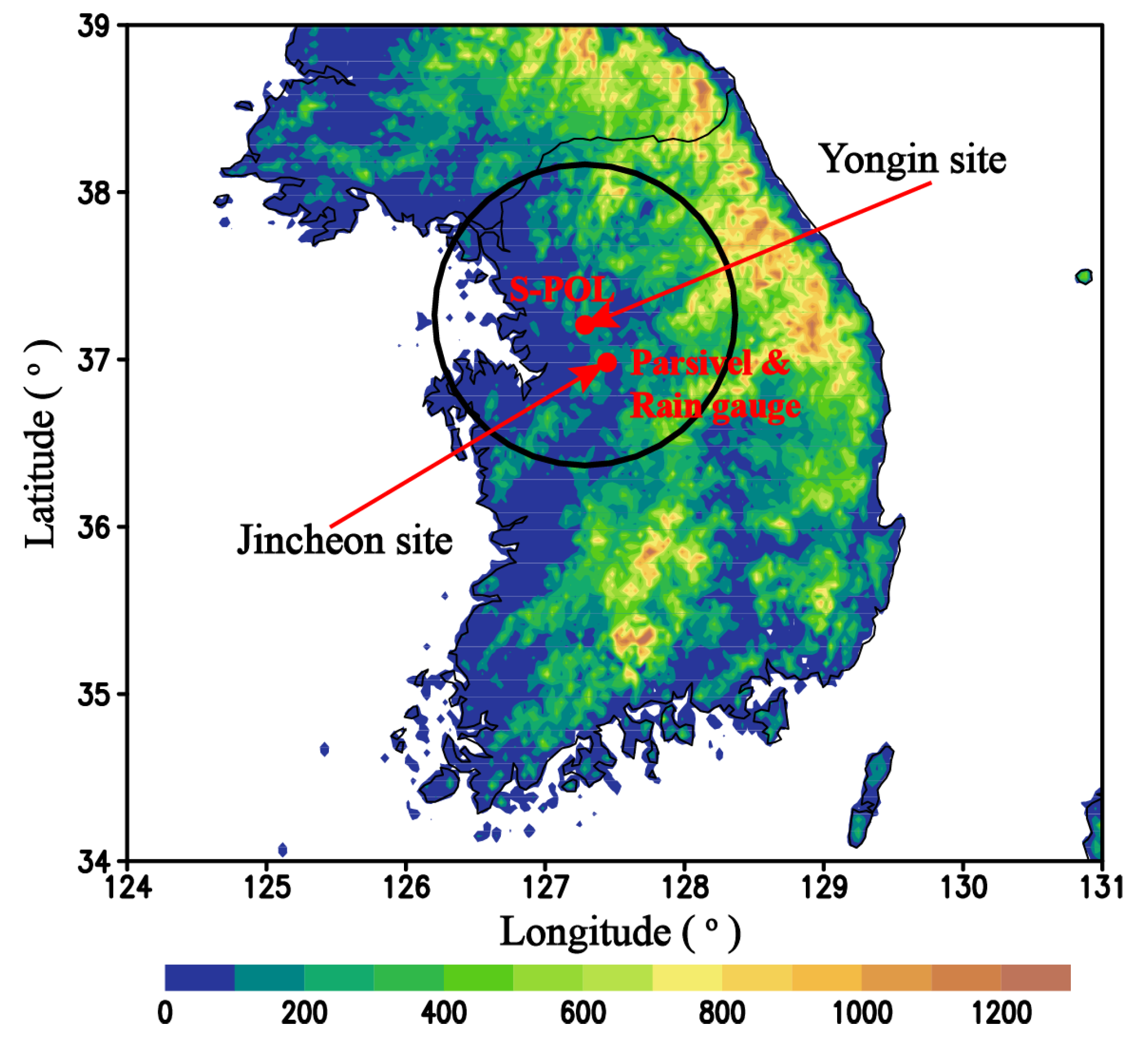
2.1. Datasets

The rain gauge, Parsivel disdrometer, and S-POL radar data from sites in Jincheon (36.98 ° N, 127.44 ° E) and Yongin (37.21 ° N, 127.29 ° E), shown in Figure 1, were acquired from June 2015 to March 2016. The rainfall data from Jincheon were collected and used to evaluate the accuracy of the radar rainfall from a tipping bucket rain gauge, which is operated and quality-controlled by the Korea Meteorological Administration (KMA). Ten days of 2015 and two days of 2016 were selected for a comparison of DSD parameters using the Parsivel disdrometer and S-POL radar, as presented in Table 1. The total daily rainfall for the 12 selected days was 385.4 mm in 155 h at the Jincheon site, and the cases were selected as those with daily rainfall larger than the threshold of 15 mm. Details can be found in Loh et al. [45].
The DSD values obtained using the Parsivel disdrometer from the Jincheon site, located 28.62 km from the S-POL radar site, were analyzed and compared with the radar retrievals in a statistical and functional approach. Briefly, the Parsivel disdrometer is a modern, laser-based optical disdrometer that measures the size and fall velocity of all liquid and solid precipitation [17,46]. It can measure 32 size bins from 0.062 to 24.5 mm [4]. A detailed description of the disdrometer can be found in Löffler-Mang and Joss [46]. A total of 17,280 1-min DSD spectra, observed from the Parsivel disdrometer for 12 days at Jincheon, were used to determine the relationship between polarimetric variables for the retrieval of DSD parameters from S-POL variables and the Parsivel disdrometer.
The S-POL radar data used in this study are from the Yongin site, operated by the Weather Radar Center of KMA (Figure 1). The S-POL radar data were updated every 10 minutes with 11 elevation angles (0.20 ° , 0.61 ° , 1.12 ° , 1.84 ° , 2.81 ° , 4.21 ° , 6.23 ° , 9.12 ° , 13.20 ° , 19.00 ° , and 80.00 ° ). The transmitted power was 850 KW, the beamwidth was 1.0 ° , the pulse repetition frequency was 599 Hz, and the effective observational range was 240 km.

2.2. Parsivel Disdrometer

2.2.1. Quality Control

The fall velocity, from Atlas et al. [47], can be defined as
v = 9.65 10.3 e 0.6 D
where v is in m s 1 , and D is the diameter of an equivalent-volume sphere, in mm, was applied to filter unreliable data. Kruger and Krajewski [48] found that the occurrence of outliers was larger as compared to Atlas et al. [47]. Therefore, a fall-velocity-based filter was developed
| V m e a s u r e d V A | < 0.4 V A
where V m e a s u r e d (m s 1 ) is the observed fall velocity and V A (m s 1 ) is v from Equation (1) used to remove the outliers of the data affected by the wind-caused turbulence [49]. In addition, 1-min rainfall rates were neglected at less than 0.1 mm h 1 (to eliminate acoustic and wind noise [8,44]) and greater than 200 mm h 1 (to enhance the capability of the detection of small raindrops (<1 mm) [44]).

2.2.2. DSD Parameters

A three-parameter ( μ , Λ , and N 0 ) normalized gamma DSD model was used in this study. The values of Λ and μ were obtained through the untruncated-moment method. The integration of most moment calculations is usually performed over the size range from zero to infinity as
D n = 0 D n N ( D ) d D = N 0 Λ ( μ + n + 1 ) Γ ( μ + n + 1 )
where n is the order and Γ ( μ + n + 1 ) is the complete gamma function [4,25]. The parameters μ , Λ , and N 0 can be obtained from any three moments (e.g., 2nd, 4th, and 6th). The ratio of the three moments, η , is defined as
η = D 4 2 D 2 D 6 = ( μ + 3 ) ( μ + 4 ) ( μ + 5 ) ( μ + 6 )
From Equation (4), the values of μ , Λ , and N 0 can be computed as
μ = ( 7 11 η ) ( 7 11 η ) 2 4 ( η 1 ) ( 30 η 12 ) 1 / 2 2 ( η 1 )
Λ = D 2 Γ ( μ + 5 ) D 4 Γ ( μ + 3 ) 1 / 2 = D 2 ( μ + 4 ) ( μ + 3 ) D 4 1 / 2
N 0 = D n Λ μ + n + 1 Γ ( μ + n + 1 )
Refs. [4,17,25,50]. Then, the value of D 0 can be obtained from μ (Equation (5)) and Λ (Equation (6)) through
D 0 = 3.67 + μ Λ
Ref. [50].
In fact, D m is very close to D 0 , which is defined as the ratio of the fourth to the third moment of the DSD:
D m = 0 N ( D ) D 4 d D 0 N ( D ) D 3 d D = D 4 D 3
The relation of D m with D 0 for a gamma distribution was also shown by Ulbrich [19] as below:
D m = 4 + μ 3 . 67 + μ D 0
The liquid water content (LWC; g m 3 ) was calculated as
L W C = π ρ w 6 0 N ( D ) D 3 d D = π 6 ρ w D 3
where ρ w (g m 3 ) is the water density [4,15,17]. The normalized intercept parameter N w (mm 1 m 3 ) is estimated from D m (Equation (10)) and LWC (Equation (11))
N w = 4 4 π ρ w L W C D m 4
Refs. [4,15,17].

2.3. S-POL Radar

2.3.1. Quality Control

The Z H and Z D R bias correction schemes were not applied but a differential phase shift ( Φ D P ) unfolding stage and noise removal stage based on study of You et al. [51] was applied. A detailed description can be found in You et al. [51]. After the noise removal from Φ D P , a specific differential phase ( K D P ) was obtained from the slope of 9 and 25 gates of quality-controlled Φ D P , with a gate size of 250 m. The lightly filtered estimate of K D P was selected when Z H 40 dBZ, whereas when Z H < 40 dBZ, the heavily filtered estimate was used for any particular range gate [51]. The calculation of the specific attenuation at horizontal polarization ( A H ) was based on the method of Ryzhkov et al. [52] and You and Lee [53]. A H can be calculated from the attenuated reflectivity ( Z a ) radial profile and two-way Path Integrated Attenuation ( P I A ) along the propagation path ( r 1 , r 2 ). Details of the A H calculation can be found in You and Lee [53].

2.3.2. DSD Parameters

The retrieval of DSD parameters from polarimetric radar is important for improving the accuracy of rainfall estimations [23]. According to Brandes et al. [23] (BRA04), Z H (mm 6 mm 3 ), Z V (mm 6 m 3 ), Z D R (dB), and K D P (deg km 1 ) are the most important factors in quantitative rain estimation among polarization radar parameters and depend on the drop scattering amplitudes and DSD. Similarly, A H (dB km 1 ) is also important and is given in terms of N ( D ) (mm 1 m 3 ) and the total extinction cross-section ( σ e ( D ) ) (mm 2 ) as described by Bringi et al. [54]. The values of Z H , Z D R , K D P , and A H can be obtained using the transition-matrix (T-matrix) scattering method, which is required to obtain information such as raindrop shape, canting angle of raindrop, frequency, temperature, and DSDs to calculate radar variables. The following raindrop shape assumptions are combined with respect to the rain drop size used for the calculation of variables from the DSDs:
b / a = 1.0048 + 0.500057 D 0.02628 D 2 + 0.003682 D 3 0.0001677 D 4
b / a = 1.012 0.01445 D 0.01028 D 2
where a, b, and D are the major axis, minor axis, and equivolume diameter of the raindrops in millimeters, respectively.
Equation (13) was proposed by Beard and Chuang [55] for the equilibrium raindrop axis ratio derived from a numerical model. Later, Andsager et al. [56] found that raindrop shapes with a diameter between 1.1 and 4.4 mm in turbulent flow are better explained by Equation (14). Bringi et al. [15] proposed the combined drop shape assumption using Equations (13) and (14) to better represent rain drops in nature. You and Lee [53] found that combining Equation (13) for raindrops smaller than 1.1 mm and larger than 4.4 mm with Equation (14) for the raindrop diameter between 1.1 and 4.4 mm gave more accurate rainfall estimates in Korea, compared with other raindrop shape assumptions. Other variables in the T-matrix calculations include the temperature, frequency and distribution of the canting angles of rain drops. The temperature is assumed to be 20 ° C, the frequency is 2.87 GHz and the distribution of their canting angles is Gaussian with a mean of 0 ° and a standard deviation of 7 ° , as determined by Huang et al. [57]. The T-matrix scattering method [58,59] was used to compute the polarimetric variables and relationships between D 0 and Z D R , and N w and Z H , using DSDs measured by a Parsivel disdrometer to determine the reference classification method for rainfall types using radar variables.

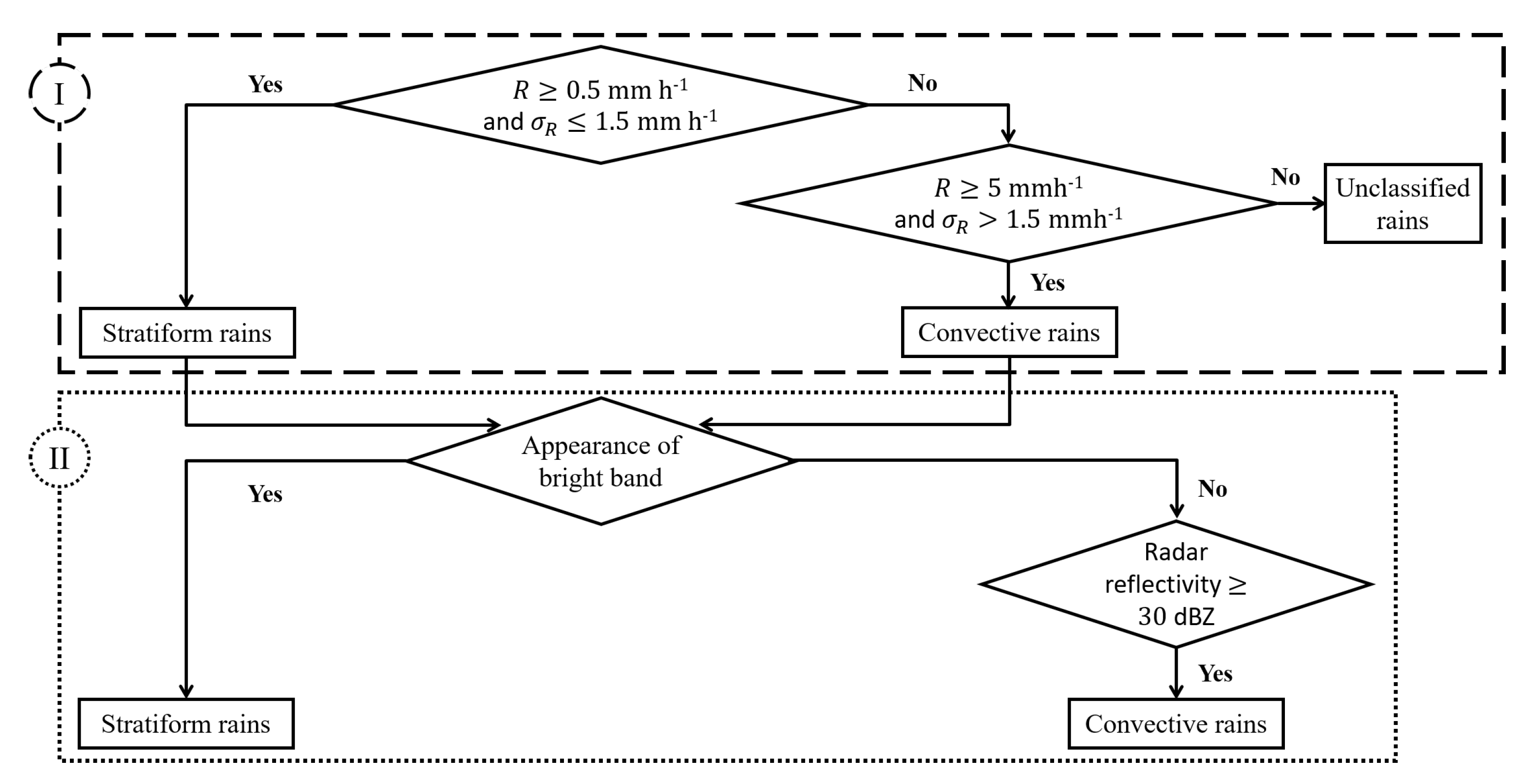
2.4. Methods for Rainfall Classification Using Disdrometer and S-POL Radar

The rain types are classified by disdrometer and S-POL radar after identification through the BR03, vertical profile of reflectivity (VPR), and BR03-VPR methods.

2.4.1. General Identification Methods

1. The BR03 method
This scheme was proposed by BR03 and has been applied in numerous studies (e.g., [17,21,39,44]). BR03 used a standard deviation for R ( σ R ) of 1.5 mm h 1 , as the threshold for the classification of convective and stratiform rains, based on data acquired by the 2DVD in Colorado, with a radar-observed bright band signature during a stratiform upslope event. For stratiform rains, the criteria were based on σ R 1.5 mm h 1 and R 0.5 mm h 1 . Otherwise, the rainfall was considered as convective rain if σ R > 1.5 mm h 1 and R 5 mm h 1 , which was adopted and conducted in every minute in this study, as shown in the dashed box (I) of Figure 2. This method is a disdrometer-based method applied to the Parsivel data. In addition, the remaining rainfall data (total samples of the Parsivel data) that belong neither to stratiform nor convective rains were categorized as unclassified rains. For the BR03 method, 1301 (382) samples of stratiform (convective) rains from the Parsivel disdrometer were selected at the Jincheon site.
2. The VPR method
The bright band is a radar signature of the melting layer, which is generally identified with stratiform rains [7,8,11]. Convective rains typically can be distinguished by considering the threshold in radar reflectivity. Almost all precipitation with a radar reflectivity above 40 dBZ was identified as convective rain (e.g., [1,2,7,8,14]), with different conditions. For instance, Steiner et al. [7] classified convective rains based on the intensity (reflectivity of at least 40 dBZ) and sharpness of the peaks of echo intensity. However, other thresholds have also been used to identify convective rains. For example, CA08 considered the rainfall as convective rain if R was greater than 10 mm h 1 , and the reflectivity was higher than 38 dBZ. A threshold of 30 dBZ was used by Niu et al. [60] to classify convective rains that resulted from the weaker precipitation system in a semi-arid continental regime [61].
Stratiform and convective rains can also be identified through the VPR method, as shown in the box II of Figure 2. This method was conducted every 10 min. Stratiform rains can be distinguished by the presence of a bright band (e.g., [1,4,7,11,18]), where the bright band was determined subjectively in this study, and rains with a reflectivity of 30 dBZ or higher are identified as convective (e.g., [60,62]) by the VPR method. According to Zhang et al. [61], the maximum height of convective rains is between 7–8 km and the height is typically 5–6 km. Franco et al. [63] introduced the 30 dBZ echo-top altitude as a discriminatory variable for classifying convective rains and indicated that a Z H value ≥ 30 dBZ at altitudes higher than 1 km can be considered as convective rains for the low-convection scenario, although the maximum height for the high-reflectivity scenario (i.e., >40 dBZ) would be the same height as that of the stratiform bright band. Therefore, weak convective rains with Z H of 30–35 dBZ at low echo-top heights (≤5 km) were also considered as convective rains in this study. The durations selected for all rainfall types at the Yongin site are summarized in Table 1.
This method is a radar-based method applied to the S-POL data. For the VPR method, 1798 (451) samples of stratiform (convective) rains were selected at Jincheon. In the current study, time series of reflectivity were analyzed to classify the different rain types at the Jincheon site (Figure 3). The vertical profiles of reflectivity (VPRs) of radar were calculated by 11 PPI scan data. The elevation angles within one volume in 10 min are 0.2, 0.6, 1.1, 1.8, 2.8, 4.2, 6.2, 9.1, 13.2, 19.0, and 80.0 degrees. Considering these elevation angles apart from 80.0 degrees and the distance between the radar and Jincheon site, the averaged vertical distance between grid points is approximately 1.12 km. Figure 3 shows the time-height cross-sections of reflectivity from the S-POL radar at the Yongin site for 12 different dates. The reflectivity values of the selected convective rains (Table 1) were larger than 35 dBZ except for 26 June 2015 (Figure 3a). The reflectivity values for 26 June 2015 were lower than for the other cases (≥35 dBZ). However, because the values occurred at ∼5 km, these were attributed to convective rains in this study. Figure 3e,f,g show that the reflectivity values of convective rains, by the S-POL radar, exceeded 45 dBZ during 0600-0610 LST and 1030-1050 LST on 2 August 2015, 1530-1620 LST on 16 August 2015, and 1410-1430 LST on 5 September 2015. In contrast, stratiform rains were selected (Table 1) by virtue of the presence of the bright band (Figure 3). Figure 3b indicates that the strong bright band was detected at a height of 4–5 km from 0900 to 1800 LST on 12 July 2015. A particularly weak-to-moderate bright band was also observed at a height of 5–6 km from 0520 to 0920 LST on 16 August 2015, at a height of 3–4 km from 1310 to 1430 LST and 1910 to 2020 LST on 7 November 2015, at a height of 2–3 km from 1900 to 2000 LST on 13 February 2016, and at a height of 2–3 km from 1630 to 1730 LST on 5 March 2016, as shown in Figure 3f,i,k,l.
3. The BR03-VPR method
A unified method, BR03-VPR, was applied in this study. The BR03-VPR combines the methods of BR03 and VPR. The VPR method may be less effective for rainfall classification owing to human error. Human error refers to the error of the individual analyst and does not correspond to the method or the procedure. Additionally, the VPR method is based on the radar data collected every 10 min, whereas the BR03 method is based on the Parsivel disdrometer data, which are updated every minute. First, the rainfall types were identified using the BR03 method (dashed box in Figure 2). Next, the rainfall types were distinguished by the appearance of the bright band and threshold values of radar reflectivity, as shown by the dotted box in Figure 2. This method was used as a reference to evaluate the accuracy of classifying rainfall types based on S-POL radar (especially for DSD retrieval and the fuzzy method as described in Section 2.4.3). A total of 1562 (1224 stratiform and 338 convective rains) 1-min DSD spectra were sampled by the BR03-VPR method in this study. The data was only selected when the resulting outputs, from previous two methods, were both identified as either stratiform or convective rains. Moreover, the DSD parameters for the Jincheon site were extracted in order to compare with the DSD retrieval and fuzzy methods.

2.4.2. Classification with DSDs Variables Measured by Parsivel Disdrometer

Several rainfall classification methods using DSD parameters acquired either from disdrometer measurements or polarimetric radar retrievals have been proposed [4]. For example, BR09 found a classification method using a relationship between D 0 and log 10 N w at Darwin, Australia. CA08 suggested a separation method for Italy that used the reflectivity and R threshold from JWD and Pludix instruments with a relationship between l o g N 0 and Λ . An empirical classification method for Kapingamarangi Atoll demonstrating log 10 N 0 R and Λ R relationships has been proposed by TS96. YOU16 developed a new classification boundary condition, based on heavy rainfall from the Parsivel disdrometer over Busan, Korea after comparing the methods of BR09, CA08, and TS96. The four separation methods, including YOU16, were compared in this study to determine an appropriate separation line for both rainfall types corresponding to the S-POL radar data.

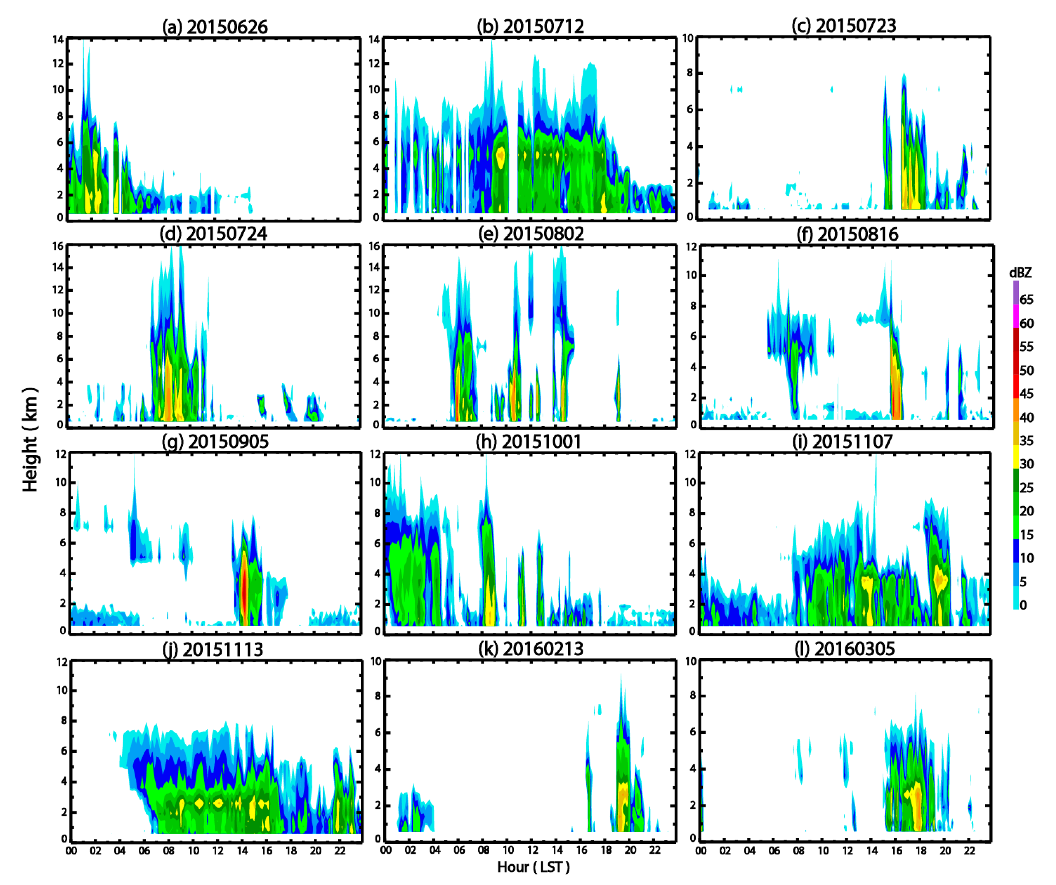
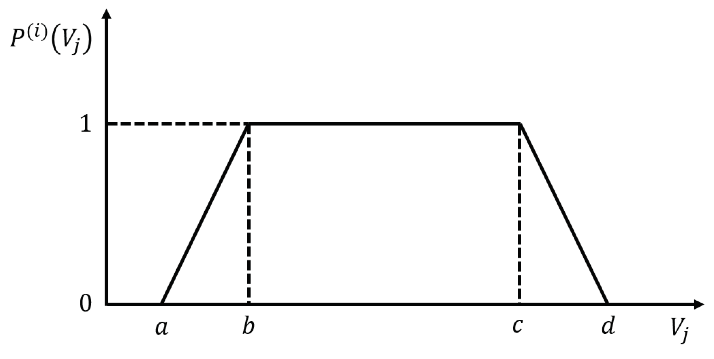
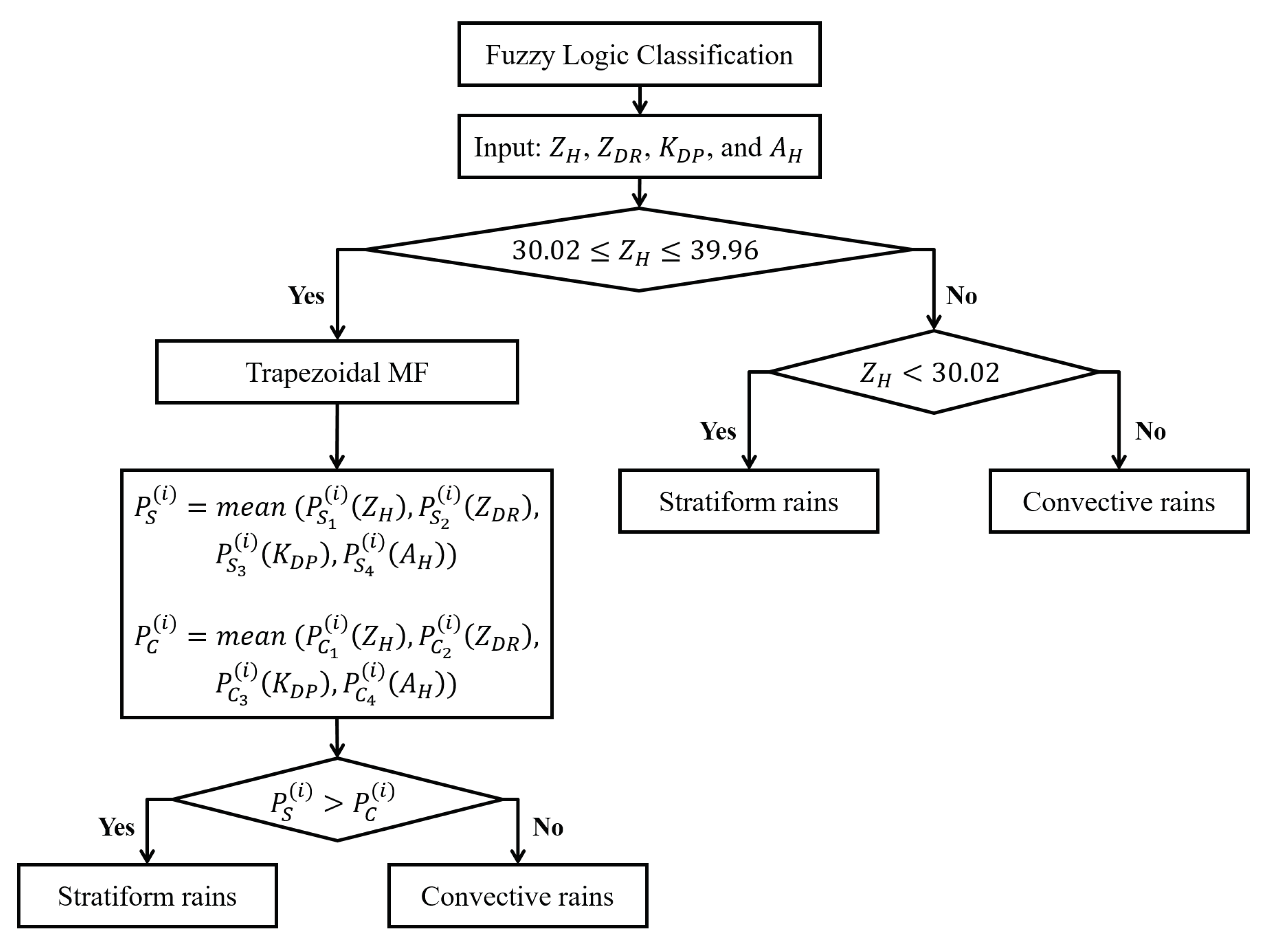
2.4.3. Classification by S-POL Radar

1. DSD retrieval method
Significant progress has been made in retrieving DSD parameters from polarimetric radar measurements, quantitatively comparing the radar retrievals with disdrometer measurements, and developing DSD models (e.g., [4,12,15,23,24,25]). Two approaches have commonly been suggested for the retrieval of a normalized gamma distribution.
The β (slope) method, proposed by Gorgucci et al. [64,65] and Bringi et al. [66] (BR02), retrieves N w and D 0 from Z H , Z D R , K D P , and β . β is given by
β = d r d D
where r is the axis ratio ( b / a ; a and b are the major and minor axes of the spheroid, respectively) and D is the equivolumetric spherical diameter in mm [64]. The goal of this method is to retrieve the DSD parameters from Z H , Z D R , K D P and β [23,64,67]. The advantage of the β method is that the three parameters of the normalized gamma DSD can be retrieved independently [67]. However, the errors in the modeled DSD and K D P estimations restrict the application of the method to cases with high R values [67], and thus the retrievals from Z H , Z D R , and K D P may be dependent [68].
The constrained-gamma method retrieves the DSD parameters based on Z H and Z D R , as proposed by Brandes et al. [23], Zhang et al. [69], Brandes et al. [70]. Brandes et al. [70] also suggested an empirical relationship ( Λ = 0.0365 μ 2 + 0.735 μ + 1.935 ), which essentially reduces the three-parameter normalized gamma DSD to a two-parameter model. Some studies have shown that the constrained-gamma method is better than the β method for DSD retrieval (e.g., [23,24,29]) despite having some uncertainties [71].
2. Fuzzy logic classification method
The fuzzy logic theory was first developed by Zadeh [72] to provide a scheme for handling issues due to the indefiniteness arising more from an intrinsic ambiguity than from a statistical variation [73]. The fuzzy set allows an element to partially belong to a set indicated by a membership degree of 0 to 1 through a membership function (MF). While 0 is defined as an element that is not included in the set at all, 1 is an element that belongs to the set [74].
Many studies have shown that a valid approach for hydrometeor classification is to use a fuzzy logic algorithm (e.g., [31,36,39,40,75]). Different hydrometeor classes were described by one-dimensional ( F ( i ) ( V j ) = P ( i ) ( V j ) , where V j is the j t h additional radar variable) or two-dimensional ( F ( i ) ( Z H , V j ) = P ( i ) ( Z H ) P Z ( i ) ( V j ) ) MFs based on the fuzzy logic methodology [76]. The one-dimensional unconditional MFs P ( i ) ( Z H ) and P Z ( i ) ( V j ) characterize distributions of Z H and V j , respectively, for the i t h class. The MFs P Z ( i ) ( V j ) characterize the conditional distribution of the variable V j for the i t h class for a given Z H . The product of P ( i ) ( Z H ) and P Z ( i ) ( V j ) represents the two-dimensional MF characterizing the joint distribution of Z H and V j in the Z V j plane for the i t h class.
The maximal aggregation value is used to identify the hydrometeor class. For each class, the aggregation was defined as
A i = j = 1 M W j F ( j ) ( Z H V j )
where M is the number of variables and W j is the weight assigned to the j t h variable [76]. Schuur et al. [76] used five radar parameters ( Z H , Z D R , co-polar correlation coefficient ( ρ H V ), a texture parameter S D ( Z H ) of the Z H field, and a texture parameter S D ( Φ D P ) of the Φ D P field) for automatic classification. Furthermore, Mahale et al. [41] identified three-body scattering by the fuzzy logic classification of S-POL radar echoes following Park et al. [31]. They defined A i as
A i = j = 1 5 W i j P ( i ) ( V j ) j = 1 5 W i j
where W i j is a weight between 0 and 1 assigned to the i t h class and j t h variable and P ( i ) ( V j ) is a trapezoidal MF for the i t h class and j t h variable. Therefore, this may be also a suitable approach for rainfall classification, as it can accurately classify the hydrometeor. However, for rainfall classification, only a few studies have classified rain types through a fuzzy logic approach (e.g., [6,26]).
The fuzzy logic approach in the current study is based on the observations of Z H , Z D R , K D P , and A H , which are highly sensitive to droplet shape, size, orientation, and composition [34,77,78,79,80], for stratiform and convective rain classification. Hence, A i can be defined as
A i = j = 1 4 W i j P ( i ) ( V j ) j = 1 4 W i j
from the Equation (17). The trapezoidal MF is defined by a < b < c < d (Figure 4), and is expressed as follows
P ( i ) ( V j ) = 0 , ( V j < a ) or ( V j > d ) V j a b a , a V j b 1 , b V j c d V j d c c V j d .
The criteria for the limits from the Parsivel data at the Jincheon site used in the trapezoidal MF are the 0.5th, 20th, 80th, and 99.5th percentiles, based on Mahale et al. [41] to obtain the values of the four limits. Details of the vertex values (a, b, c, and d) are shown in Table A1 and Table A2.
Figure 5 shows a flowchart classifying stratiform and convective rains through the trapezoidal MF using S-POL radar data from the Yongin site. The radar classification with the trapezoidal MF method can be performed after obtaining the values of the four limits from the Parsivel data. First, the stratiform rains can be identified when Z H < 30.02 dBZ, whereas the convective rains can be verified if Z H > 39.96 dBZ. According to Hwang [81], the summation of inputs for the fuzzy logic method is advantageous, because other inputs can compensate, particularly for the cases that have weak characteristics in one input. Hence, this summation of inputs is applied in the current study for the intercept of Z H between 30.02 and 39.96 dBZ (Figure 5). The stratiform rains can be identified if P S ( i ) (mean value of the input summation for stratiform rains) is larger than P C ( i ) (mean value of the input summation for convective rains); otherwise, the classification is convective rain. Details of the trapezoidal MF classification method are shown in Figure 5.

3. Results

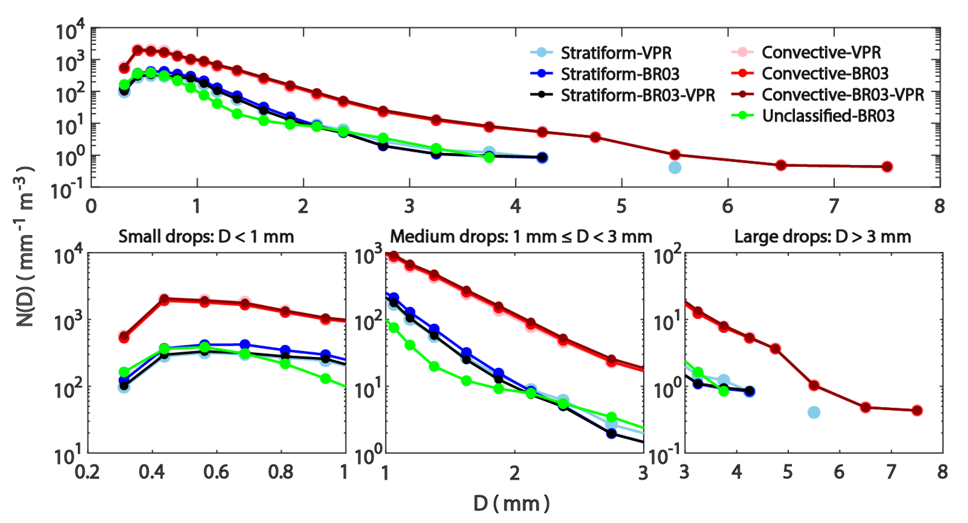
3.1. The Characteristics of DSDs

The averaged droplet number concentration of each rain type during the selected period (Table 1) are shown in Figure 6. Notably, all the convective rains of the three different methods (VPR, BR03, and BR03-VPR) contain more raindrops than the other types (stratiform and unclassified rains) across all drop sizes. Furthermore, stratiform and unclassified rains were found to have a similar pattern, but with minor differences in magnitude, particularly for small drops (0.31–0.65 mm), as shown in the bottom left panel of Figure 6. The DSDs were distributed in a concave downward manner and shifted toward larger drops for more abundant forms in all the rainfall types. The peak number concentration of all convective rains occurred at 0.44 mm, whereas almost all the stratiform rains showed a peak number concentration of 0.56 mm, except for the BR03 method (0.69 mm). This behavior is probably due to the dead time problem of the disdrometer originating from the insensitivity of the instrument to small drops [16,45].
The mean R (mean D) were 1.98 mm h 1 (1.67 mm), 24.43 mm h 1 (2.34 mm), and 0.41 mm h 1 (1.41 mm) for the averaged stratiform rains of the three different methods (VPR, BR03, and BR03-VPR), averaged convective rains (same methods), and unclassified rains of the BR03 method, respectively. The maximum log 10 N w of the stratiform rains (5.10 mm 1 m 3 ) was higher than that of the convective rains (4.93 mm 1 m 3 ) in the BR03 method (Table 2). This might have occurred when large drops formed below the bright band in the stratiform rains [4]. However, Moreover, the mean of the entire dataset was less than that of the convective rains, as the stratiform rains had an abundance of small drops. Furthermore, the DSD of the convective rains ( D m a x = 7.50 mm) was much broader than that of the stratiform rains ( D m a x = 4.25 mm).

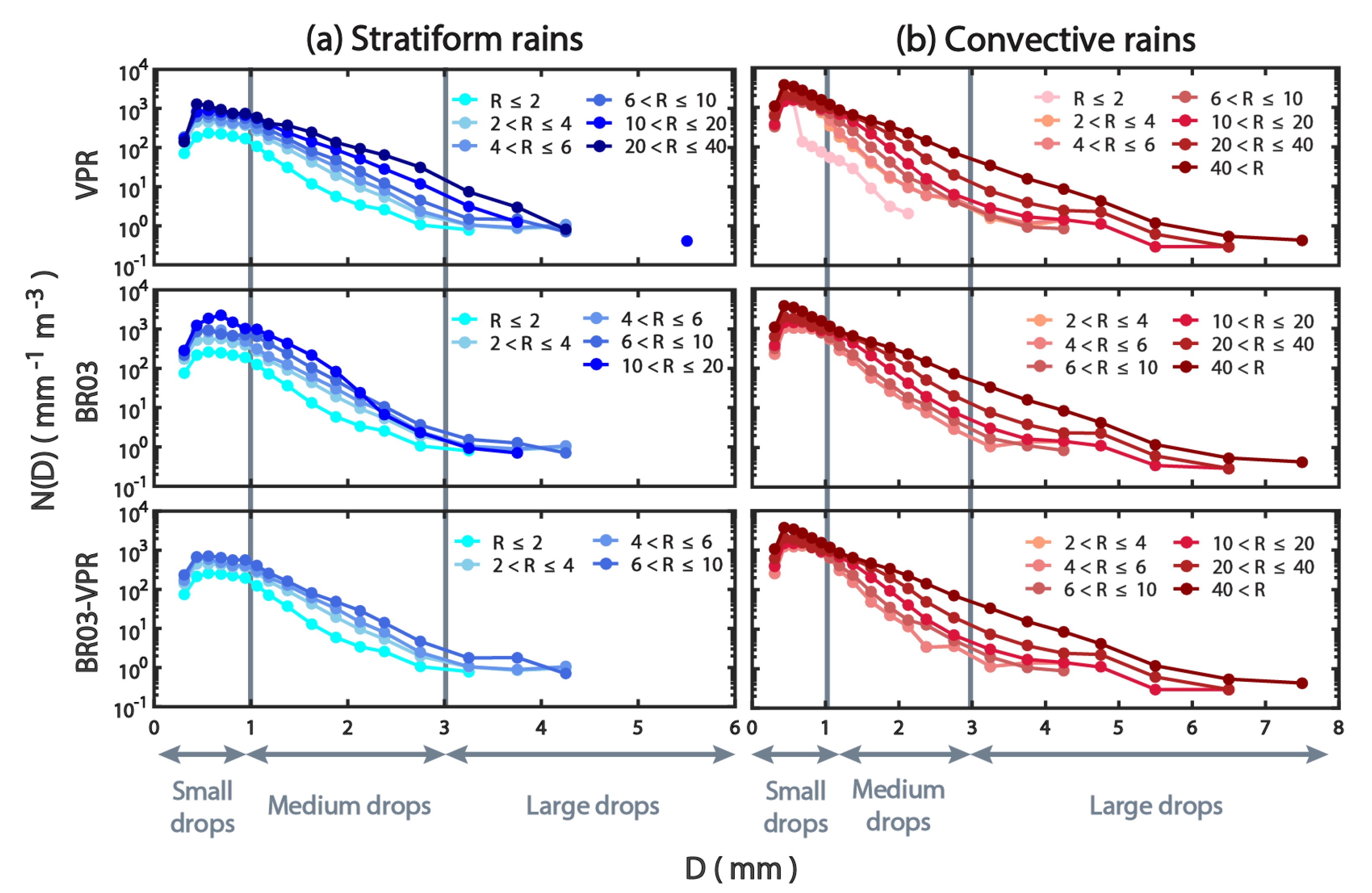
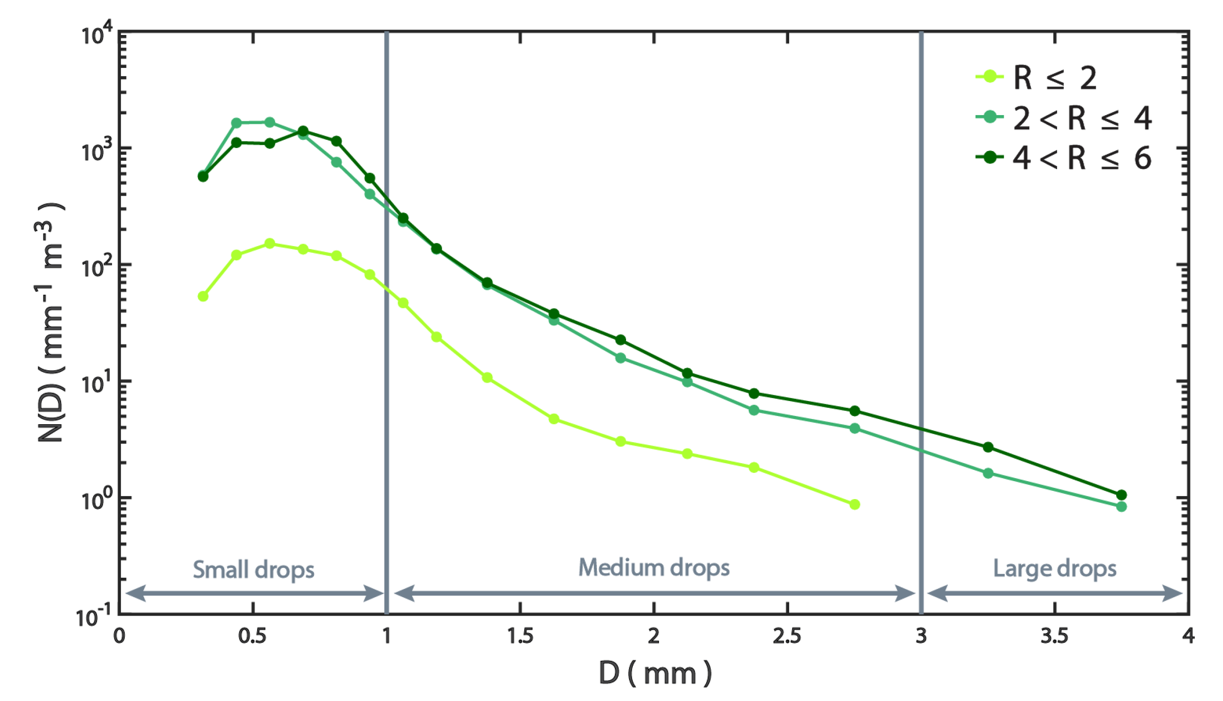
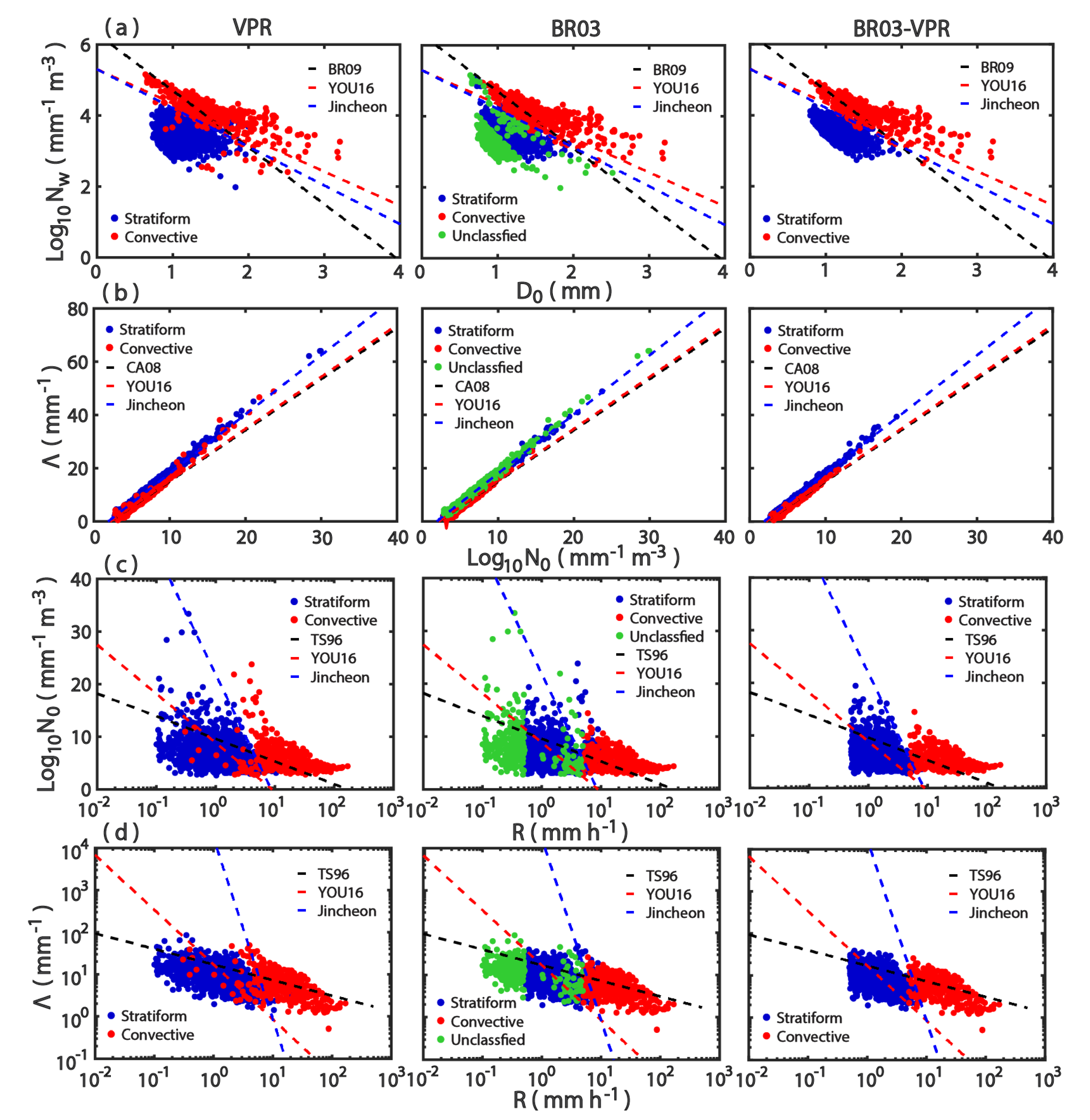
3.2. Relationship between DSD and R

Figure 7 shows the average DSDs of the different R classes for stratiform and convective rains. The number of rainfall categories for the stratiform rains (six classes: R 2 mm h 1 , 2 < R 4 mm h 1 , 4 < R 6 mm h 1 , 6 < R 10 mm h 1 , 10 < R 20 mm h 1 , and 20 < R 40 mm h 1 ) was lower than that for the convective rains (seven classes: R 2 mm h 1 , 2 < R 4 mm h 1 , 4 < R 6 mm h 1 , 6 < R 10 mm h 1 , 10 < R 20 mm h 1 , 20 < R 40 mm h 1 , and R > 40 mm h 1 ). The convective rains had higher R ( R > 40 mm h 1 ) than the stratiform rains. Moreover, the R values for all the stratiform rains were found to be in the lowest category ( R 2 mm h 1 ), as shown in Figure 7a. However, only the VPR method existed for the convective rains (Figure 7b). It was expected that the R of the stratiform rains would be lower than that of the convective rains (e.g., [14,82]).
For the VPR method, the number concentration increased with R only when 1.06 < D 3.75 mm for the stratiform rains. In contrast, the number concentration in the convective rains increased with R only when 1.06 < D 2.38 mm and D ≥ 4.75 mm. For the BR03 method, the number concentration in the convective rains increased for all diameter bins when R increased for smaller drops ( D < 1 mm), whereas for medium drops (1 D < 3 mm), almost all types showed an increase in number concentration for all diameter bins with increasing R for the stratiform and convective rains. Finally, for the BR03-VPR method, the number concentration of the stratiform rains increased with R only when D ≤ 3.75 mm, whereas for the convective rains, the number concentration increased with R only when 1.06 < D 3.25 mm and D ≥ 4.75 mm.
For stratiform rains, the BR03-VPR method showed that the average drop size spectra increased with increasing R across small and medium drops. Furthermore, for medium drops, the VPR method of the stratiform rains showed that average DSDs increased with increasing R. However, for the convective rains, the BR03 method showed that the average drop size spectra increased with increasing R across small and medium drops. In addition, all the methods of the convective rains indicated that the average DSDs increased with increasing R across all the diameter bins for medium drops, except for the VPR method. Figure 8 presents the size distribution of the unclassified rains. The figure demonstrates the average DSDs according to three classes ( R 2, 2 < R 6, and 4 < R 6) for the unclassified rains according to the BR03 method over small, medium, and large drops. The number concentration increased with increasing R only when the diameter in the ranges D ≥ 0.69 mm.

3.3. Comparison of Rainfall Classification

3.3.1. Parsivel Disdrometer

Figure 9a shows scatter plots of the measurements of log 10 N w against D 0 along with the classification lines proposed by BR09, YOU16, and the new separation line derived from the Jincheon site. The values of D 0 ( log 10 N w ) for stratiform rains of all methods ranged from 0.72 mm (1.97 mm 1 m 3 ) to 1.99 mm (5.10 mm 1 m 3 ). The corresponding ranges for all convective rains were 0.64 mm (2.41 mm 1 m 3 ) to 3.20 mm (5.16 mm 1 m 3 ). However, the classification lines of BR09 and YOU16 failed to separate the stratiform and convective rains correctly for all three methods (VPR, BR03, and BR03-VPR). The YOU16 classification line seems to provide a better separation than BR09 (Table 3), which may be because the rainfall types are from the same weather systems. Table 3 shows the percentages of misclassification of both rainfall types based on the D 0 log 10 N w , log 10 N 0 Λ , R log 10 N 0 , and Λ R separation lines.
The BR09 classification line separated the stratiform rains better (with a misclassification of 0.00% to 1.61%) than the convective rains (with a misclassification of 23.67% to 36.14%). Hence, a new classification line was proposed for the Jincheon site based on visual examination to separate the stratiform and convective rains more accurately,
log 10 N w = 1.09 D 0 + 5.3 .
The Jincheon separation line (blue line in Figure 9a) could classify both rainfall types more accurately compared with BR09 and YOU16 for all three methods. Table 3 also demonstrates that the Jincheon separation line performed better than the others, with lower misclassification rates for both stratiform (1.23–6.99%) and convective (1.78–5.76%) rains. The BR03-VPR method had the lowest misclassification rates for stratiform and convective rains, at 1.23% and 1.78%, respectively among the three methods.
Figure 9b shows scatter plots of log 10 N 0 versus the slope parameter ( Λ ), which referred to the CA08 study. In general, the CA08 and YOU16 classification lines failed to separate the stratiform and convective rains. Table 3 also shows the high degree of misclassification, especially for convective rains, at ∼53% for the VPR, BR03, and BR03-VPR methods. The proposed classification line is very similar to that presented for CA08 and YOU16, based on the visual judgement of the Jincheon data, as shown below
Λ + 4.17 = 2.22 log 10 N 0 .
However, the Jincheon separation line also failed to classify both rainfall types at the Jincheon site. It is difficult to accurately derive the log 10 N 0 Λ relationship because of the overlapping of stratiform and convective rains, as shown in Figure 9b. YOU16 indicated that it is not possible to cleanly classify the convective and stratiform rains because of the overlapping in log 10 N 0 Λ space. Additionally, they also proposed that the log 10 N 0 Λ domain by the CA08 classification line is unsuitable for Korea.
The scatter plots of log 10 N 0 against R for the Jincheon site are shown in Figure 9c. The R values for the stratiform and convective rains were in the ranges of 0.0–27.5 and 0.0–169.8 mm h 1 , respectively, for the VPR method. For the BR03 and BR03-VPR methods, the R for the stratiform and convective rains were in the ranges of 0.5–14.6 and 5.0–169.8 mm h 1 , respectively. Moreover, the values of log 10 N w for the stratiform and convective rains were in the ranges of 2.7–33.4 and 2.8–23.8 mm 1 m 3 , respectively. The TS96 and YOU16 classification lines failed to separate the stratiform and convective rains (Figure 9c). Table 3 also shows that the YOU16 separation line could classify the stratiform rains better than the TS96 classification line. Hence, a new separation line was created for the Jincheon site to accurately classify the two rain types. The Jincheon separation line based on visual examination is shown below
N 0 = 7 × 10 21 R 23.3 .
The newly derived separation lines (Equation (22)) were able to clearly separate the stratiform and convective rains. Table 3 also demonstrates that the Jincheon separation line performed better with lower misclassification rates, especially for stratiform rains (3.35–8.76%). The BR03-VPR method had the lowest misclassification rates of 1.18% and 3.35% for convective and stratiform rains, respectively.
Figure 9d presents scatterplots of Λ against R for the Jincheon site. Again, TS96 and YOU16 failed to classify the two rain types. The YOU16 separation line classified the rainfall types better than TS96 because of the different microphysical processes of different regions, as the TS96 separation line is applied to the rainfall in the Kapingamarangi Atoll [4]. Table 3 also indicates that the TS96 and YOU16 classification lines had higher misclassification rates, especially for convective rains. Thus, the newly proposed separation line based on the visual examination of the data is
Λ = 17 × 10 3 R 4.3 .
Equation (23) accurately separates the stratiform and convective rains, particularly for the BR03-VPR method. This method had the lowest misclassification rates of 0.90% and 5.03% for stratiform and convective rains, respectively. The new proposed classification line could accurately separate the stratiform and convective rains for all of the relationships, except for the log 10 N 0 Λ space. The proposed R log 10 N 0 classification line was able to accurately classify the convective rains, whereas for the stratiform rains, the D 0 log 10 N w classification line was suitably accurate. The DSD parameters D 0 and log 10 N w were retrieved from the S-POL radar for the classification of rainfall types as N w and D 0 can be retrieved from polarimetric variables.

3.3.2. S-POL Radar

1. DSD retrieval
Data from all 12 days were used to classify the rainfall types using the S-POL radar. YOU16 indicated that the type of rainfall event occurring over Korea can be assumed by the values of R, D 0 , log 10 N w , Z H , and Z D R . The mean, minimum, and maximum R are 0.80, 0.003, and 49.0 mm h 1 , respectively. Furthermore, the values of D 0 ( log 10 N w ) were found to be in the ranges of 0.38–4.29 mm (1.02–5.41 mm 1 m 3 ). The Z D R ( Z H ) values ranged between 0.001 and 3.922 dB (3.94–55.58 dBZ). The D 0 Z D R and D 0 Z H N w relationships were established using the DSD measurements to derive D 0 and Z D R from the S-POL radar (Figure 10). D 0 was significantly positively correlated with Z D R , yielding a correlation coefficient of 0.78 (Table 4). The following equation was derived as
D 0 = 1.39 Z D R 0.235
(Figure 10a).
Figure 10b shows the scatter plots of Z H N w versus D 0 as well as the curves fitted to the data, as proposed by BR09 and YOU16. The newly derived equations for the Jincheon site seem more accurate, as displayed in Figure 10b. The new power-law relations have the same coefficient as YOU16, but with different magnitudes in the exponent, as shown below
Z H N w = 0.035 D 0 6.655 .
However, Table 4 shows that the relationship between Z H N w D 0 was not as strong as the relationship between D 0 and Z D R . Further studies on the relationship between Z H N w and D 0 are needed for a more detailed understanding.
BRA04 indicated that the enabling of correlations between DSD parameters for DSD retrieval from a pair of independent remote measurements such as Z H and Z D R , is useful for reducing the number of unknowns. They proposed a polynomial fit equation for Florida DSD data during the summer of 1998. Hence, a new polynomial fit
D 0 = 0.155 Z D R 3 0.897 Z D R 2 + 1.851 Z D R + 0.576
was obtained, as shown in Figure 11. Nonetheless, D 0 was highly correlated with Z D R , yielding correlation coefficients of 0.81 (Table 4). Table 4 also shows that D 0 had a stronger correlation with Z D R as compared to BRA04.
2. Fuzzy logic classification
All parameters had positively skewed distributions for both rain types (Figure 12). The skewness for convective rains was higher than that for stratiform rains, except for Z D R . The skewness was the largest for the K D P distribution for convective rains, at 2.85. This was followed by the skewness values of 2.71, 1.41, and 0.44 for the convective rains of A H , Z D R , and Z H , respectively. Similarly, for stratiform rains, the distribution of K D P had the highest skewness as compared to the others, followed by the skewness values of 1.71, 1.54, and 0.33 for the convective rains of Z D R , A H , and Z H , respectively. The Z H value (Figure 12a) showed that Z H < 29.30 dBZ indicated stratiform rains, and Z H > 37.42 dBZ indicated convective rains.
Figure 12b also shows that stratiform rains can be identified when Z D R < 0.19 dB, whereas convective rains correspond with Z D R > 1.13 dB. For K D P , stratiform and convective rains can also be identified when K D P < 0.034 and K D P > 0.098 deg km 1 , respectively. Also, the presence of convective rains can be confirmed when A H > 0.0022 dB km 1 , and rains are classified as stratiform when A H < 0.0015 dB km 1 . The trapezoidal MF can identify stratiform and convective rains easily and effectively, especially for Z H . However, clearly distinguishing both rain types only by way of the intercept is difficult. Therefore, the same steps are applied again for the intercepts of all the DSD parameters based on the interval of Z H , where 30 Z H < 40, as shown in Figure 12. Figure 13 displays the trapezoidal MF and distribution of Z H , Z D R , K D P , and A H based on 30 Z H < 40 for both stratiform and convective rains, through the BR03-VPR method. Again, all the parameters had positively skewed distributions for convective and stratiform rains, as shown in Figure 13. The trapezoidal MF for Z H , K D P , and A H has a clear triangular intercept.
3. Comparison
Three different methods were compared in this study. The first method was given by SHY95, which is based on the analysis of the horizontal gradient of the radar reflectivity field. The method considers rains as convective if Z H 40 dBZ or greater than the fluctuating threshold, depending on the area-averaged background reflectivity for any grid point within the radar scan radius. The DSD retrieval method uses Equations (25) and (26) to calculate the retrieved N w and D 0 , respectively, as retrieved from the observed Z H and Z D R of S-POL radar. The third method of classification, the fuzzy method, has also compared in this section.
For example, during 26 June 2015 from 0130 to 0200 LST (not shown), the SHY95 method failed to identify the convective rains at the Jincheon site, unlike the DSD retrieval and fuzzy methods. This may be because the classification criteria for SHY95 are not suitable to Korea. However, DSD retrieval and fuzzy methods can classify the convective rains with a similar pattern at the Jincheon site. Table 5 displays a comparison of the precision for stratiform and convective rain classification in percentages with the three different methods from the S-POL radar, for all 12 cases that were selected. For the stratiform rains, all the methods classify the rains, particularly the SHY95 method, with 85.47% for stratiform and 0.00% for convective rains. In contrast, the DSD retrieval method showed the lowest (higher) percentages, 61.45% (24.02%) for the appearance stratiform (convective) rains. The new fuzzy method for stratiform rains performed well with 79.61% of stratiform rains and 5.87% of convective rains, which is as good as the SHY95 method.
Meanwhile, the DSD retrieval method had a higher percentage (68.83%) for the convective rains as compared with the others (64.71 and 22.55% for the fuzzy and SHY95 methods, respectively). Table 5 shows that improvement in the fuzzy method is almost thrice that of the SHY95 method for convective rains classification. For the S-POL radar, the fuzzy method seems to identify better than the SHY95 and DSD retrieval methods, especially for the stratiform rains, with a missclassification rate of 5.87%. Hence, the fuzzy method can be considered suitable for classifying the rainfall types at the Jincheon site for all 12 cases that were selected. The fuzzy method performs the best classification for stratiform and convective rains in this study.

4. Conclusions

The aim of this study was to compare the existing classification methods by using Parsivel and S-POL data and to propose a new separation method for central South Korea after classification. Two identification methods of stratiform and convective rains were applied, namely BR03 and VPR, and a new unified method (BR03-VPR) was introduced for rainfall in Korea based on Parsivel disdrometer data. Generally, the BR09, YOU16, and TS96 classification methods could be applied in this study if the slope and/or intercept of the equations were altered. The newly developed separation lines performed well at the Jincheon site using DSD parameters, except for the relationship between log 10 N 0 and Λ . The best-fit line could not be obtained for the Jincheon site using the CA08 method, just as in the study of YOU16.
Three methods (SHY95, DSD retrieval, and fuzzy methods) were used to classify two rain types by the S-POL radar from the Yongin site. Briefly, SHY95 is based on Steiner et al. [7], wheares the DSD retrieval method retrieves the N w and D 0 parameters according to BRA04 and BR09. The three different methods were compared for the Korean rainfall classification. For the stratiform rain classification, SHY95 was found to be the best method, with 0.00% misclassification, whereas the DSD retrieval method was the foremost method for convective rain classification, with 30.39% misclassification. The fuzzy method performs better than the SHY95 and DSD retrieval methods, with 5.87% and 34.31% misclassification for the stratiform and convective rains, respectively. Hence, it can be concluded that the new fuzzy method can classify stratiform and convective rains more accurately as compared with the DSD retrieval and SHY95 methods, even though only 12 cases were used in this study. The fuzzy method performs the best classification for stratiform and convective rains in this study.
Finally, it is suggested that the rainfall identification should be conducted using the new unified BR03-VPR method. This method is more accurate in classifying the rain types for both disdrometer and radar data. For the Parsivel disdrometer, the newly obtained classification line D 0 log 10 N w from DSD data would be the best classification method for central South Korea. The fuzzy method was found to be more effective in classifying the rain types for S-POL radar from central South Korea. In future studies, the characteristics of DSDs for different rainfall systems and at different locations in South Korea will be examined to gain further understanding of the microphysical characteristics of the Korean rainfall system. This method can potentially be used to characterize rainfall type in any region of the world with a different coefficient, which depending on the different characteristics of the DSD. The accumulation of DSD data according to the rainfall types is very important for microphysical understanding and also radar calibration as well as Numerical Weather Forecast validation using radar data.

Author Contributions

The work presented here was carried out in collaboration with all authors. J.L.L. produced the manuscript, performed the experiments and data analysis, and contributed to the revising of the manuscript; D.-I.L., M.-Y.K. and C.-H.Y. participated in discussions on the results; C.-H.Y. contributed to the conception, reviewing and revising of the manuscript. D.-I.L. and C.-H.Y. supervised the work and provided critical comments. All authors have read and agreed to the published version of the manuscript.

Funding

This work was funded by the Korea Meteorological Industry Promotion Agency under Grant KMI 2018-05410.

Acknowledgments

The authors would like to thank the Korea Meteorological Administration for providing the Parsivel and radar data used in this study.

Conflicts of Interest

The authors declare no conflict of interest.

Abbreviations

The following abbreviations are used in this manuscript:
2DVD2-Dimensional Video Disdrometer
BR02Bringi et al. [66]
BR03Bringi et al. [15]
BR03-VPRBringi et al. [15]-vertical profile of reflectivity
BR09Bringi et al. [12]
BRA04Brandes et al. [23]
CA08Caracciolo et al. [16]
DSDsDrop size distributions
JWDJoss-Waldvogel disdrometer
KMAKorea Meteorological Administration
LWCLiquid water content
MFMemebership Function
ParsivelPARticle SIze and VELocity
PIAPath Integrated Attenuation
PludixX-band pluvio-disdrometer
S-POLS-band polarimetric
SHY95Steiner et al. [7]
STDStandard deviation
T-matrixTransition-matrix
TS96Tokay and Short [8]
VPRVertical profile of reflectivity
YOU16You et al. [4]

Appendix A

The four vertex values of trapezoidal MF (a, b, c, and d) were shown in Table A1 and Table A2 for overall and intercept of Z H between 30 and 40 dBZ, respectively as presented in Figure 12 and Figure 13.
Table A1. The vertex values of the trapezoidal MF for Z H (dBZ), Z D R (dB), K D P (deg km 1 ), and A H (dB km 1 ) as presented in Figure 12.
Stratiform RainsConvective Rains
Z H Z D R K D P A D R Z H Z D R K D P A D R
(dBZ)(dB)(deg km 1 )(dB km 1 )(dBZ)(dB)(deg km 1 )(dB km 1 )
a (0.5th)17.950.150.0030.000229.300.190.0340.0015
b (20th)22.250.250.0060.000335.410.400.0950.0030
c (80th)30.180.510.0270.000946.131.230.6320.0110
d (99.5th)37.421.130.0980.002255.473.003.7730.0502
Table A2. Same as Table A1, but for intercept of Z H between 30 and 40 dBZ as presented in Figure 13.
Stratiform RainsConvective Rains
Z H Z D R K D P A H Z H Z D R K D P A H
(dBZ)(dB)(deg km 1 )(dB km 1 )(dBZ)(dB)(deg km 1 )(dB km 1 )
a (0.5th)30.020.350.0220.000530.310.210.0380.0014
b (20th)30.940.480.0300.000934.050.330.00770.0024
c (80th)34.070.780.00550.001438.680.650.1700.0051
d (99.5th)38.031.440.1110.002439.961.530.2510.0083

References

  1. Anagnostou, E.N. A convective/stratiform precipitation classification algorithm for volume scanning weather radar observations. Meteorol. Appl. 2004, 11, 291–300. [Google Scholar] [CrossRef]
  2. Penide, G.; Kumar, V.V.; Protat, A.; May, P.T. Statistics of drop size distribution parameters and rain rates for stratiform and convective precipitation during the North Australian wet season. Mon. Weather Rev. 2013, 141, 3222–3237. [Google Scholar] [CrossRef]
  3. Penide, G.; Protat, A.; Kumar, V.V.; May, P.T. Comparison of two convective/stratiform precipitation classification techniques: Radar reflectivity texture versus drop size distribution–based approach. J. Atmos. Ocean. Technol. 2013, 30, 2788–2797. [Google Scholar] [CrossRef]
  4. You, C.H.; Lee, D.I.; Kang, M.Y.; Kim, H.J. Classification of rain types using drop size distributions and polarimetric radar: Case study of a 2014 flooding event in Korea. Atmos. Res. 2016, 181, 211–219. [Google Scholar] [CrossRef]
  5. Anagnostou, E.N.; Kummerow, C. Stratiform and convective classification of rainfall using SSM/I 85-GHz brightness temperature observations. J. Atmos. Ocean. Technol. 1997, 14, 570–575. [Google Scholar] [CrossRef]
  6. Yang, Y.; Chen, X.; Qi, Y. Classification of convective/stratiform echoes in radar reflectivity observations using a fuzzy logic algorithm. J. Geophys. Res. Atmos. 2013, 118, 1896–1905. [Google Scholar] [CrossRef]
  7. Steiner, M.; Houze, R.A., Jr.; Yuter, S.E. Climatological characterization of three-dimensional storm structure from operational radar and rain gauge data. J. Appl. Meteorol. 1995, 34, 1978–2007. [Google Scholar] [CrossRef]
  8. Tokay, A.; Short, D.A. Evidence from tropical raindrop spectra of the origin of rain from stratiform versus convective clouds. J. Appl. Meteorol. 1996, 35, 355–371. [Google Scholar] [CrossRef] [Green Version]
  9. Kitchen, M.; Brown, R.; Davies, A. Real-time correction of weather radar data for the effects of bright band, range and orographic growth in widespread precipitation. Q. J. R. Meteorol. Soc. 1994, 120, 1231–1254. [Google Scholar] [CrossRef]
  10. Awaka, J.; Iguchi, T.; Okamoto, K. TRMM PR standard algorithm 2A23 and its performance on bright band detection. J. Meteorol. Soc. Japan. Ser. II 2009, 87, 31–52. [Google Scholar] [CrossRef] [Green Version]
  11. Biggerstaff, M.I.; Listemaa, S.A. An improved scheme for convective/stratiform echo classification using radar reflectivity. J. Appl. Meteorol. 2000, 39, 2129–2150. [Google Scholar] [CrossRef]
  12. Bringi, V.; Williams, C.; Thurai, M.; May, P. Using dual-polarized radar and dual-frequency profiler for DSD characterization: A case study from Darwin, Australia. J. Atmos. Ocean. Technol. 2009, 26, 2107–2122. [Google Scholar] [CrossRef]
  13. Thurai, M.; Bringi, V.; May, P. CPOL radar-derived drop size distribution statistics of stratiform and convective rain for two regimes in Darwin, Australia. J. Atmos. Ocean. Technol. 2010, 27, 932–942. [Google Scholar] [CrossRef]
  14. Thompson, E.J.; Rutledge, S.A.; Dolan, B.; Thurai, M. Drop size distributions and radar observations of convective and stratiform rain over the equatorial Indian and West Pacific Oceans. J. Atmos. Sci. 2015, 72, 4091–4125. [Google Scholar] [CrossRef]
  15. Bringi, V.; Chandrasekar, V.; Hubbert, J.; Gorgucci, E.; Randeu, W.; Schoenhuber, M. Raindrop size distribution in different climatic regimes from disdrometer and dual-polarized radar analysis. J. Atmos. Sci. 2003, 60, 354–365. [Google Scholar] [CrossRef]
  16. Caracciolo, C.; Porcu, F.; Prodi, F. Precipitation classification at mid-latitudes in terms of drop size distribution parameters. Adv. Geosci. 2008, 16, 11–17. [Google Scholar] [CrossRef] [Green Version]
  17. Tang, Q.; Xiao, H.; Guo, C.; Feng, L. Characteristics of the raindrop size distributions and their retrieved polarimetric radar parameters in northern and southern China. Atmos. Res. 2014, 135, 59–75. [Google Scholar] [CrossRef]
  18. Uijlenhoet, R.; Steiner, M.; Smith, J.A. Variability of raindrop size distributions in a squall line and implications for radar rainfall estimation. J. Hydrometeorol. 2003, 4, 43–61. [Google Scholar] [CrossRef]
  19. Ulbrich, C.W. Natural variations in the analytical form of the raindrop size distribution. J. Appl. Meteorol. Climatol. 1983, 22, 1764–1775. [Google Scholar] [CrossRef] [Green Version]
  20. Rosenfeld, D.; Ulbrich, C.W. Cloud microphysical properties, processes, and rainfall estimation opportunities. Radar Atmos. Sci. Collect. Essays Honor. David Atlas 2003, 52, 237–258. [Google Scholar]
  21. Chen, B.; Yang, J.; Pu, J. Statistical characteristics of raindrop size distribution in the Meiyu season observed in eastern China. J. Meteorol. Soc. Japan. Ser. II 2013, 91, 215–227. [Google Scholar] [CrossRef] [Green Version]
  22. Chandrasekar, V.; Meneghini, R.; Zawadzki, I. Global and local precipitation measurements by radar. In Radar and Atmospheric Science: A Collection of Essays in Honor of David Atlas; American Meteorological Society: Boston, MA, USA, 2003; pp. 215–236. [Google Scholar]
  23. Brandes, E.A.; Zhang, G.; Vivekanandan, J. Comparison of polarimetric radar drop size distribution retrieval algorithms. J. Atmos. Ocean. Technol. 2004, 21, 584–598. [Google Scholar] [CrossRef] [Green Version]
  24. Brandes, E.A.; Zhang, G.; Vivekanandan, J. Drop size distribution retrieval with polarimetric radar: Model and application. J. Appl. Meteorol. 2004, 43, 461–475. [Google Scholar] [CrossRef] [Green Version]
  25. Vivekanandan, J.; Zhang, G.; Brandes, E. Polarimetric radar estimators based on a constrained gamma drop size distribution model. J. Appl. Meteorol. 2004, 43, 217–230. [Google Scholar] [CrossRef] [Green Version]
  26. Mesnard, F.; Pujol, O.; Sauvageot, H.; Costes, C.; Bon, N.; Artis, J.P. Discrimination between convective and stratiform precipitation in radar-observed rainfield using fuzzy logic. In Proceedings of the 5th European Conference on Radar in Meteorology and Hydrology (ERAD 2008), Helsinki, Finland, 30 June–4 July 2008. [Google Scholar]
  27. Steiner, M.; Houze, R. Three-dimensional validation at TRMM ground truth sites: Some early results from Darwin, Australia. In Proceedings of the 26th International Conference on Radar Meteorology, Norman, OK, USA, 24–28 May 1993; pp. 417–420. [Google Scholar]
  28. Bringi, V.N.; Chandrasekar, V.; Xiao, R. Raindrop axis ratios and size distributions in Florida rainshafts: An assessment of multiparameter radar algorithms. IEEE Trans. Geosci. Remote Sens. 1998, 36, 703–715. [Google Scholar] [CrossRef] [Green Version]
  29. Anagnostou, M.N.; Anagnostou, E.N. Performance of algorithms for rainfall retrieval from dual-polarization X-band radar measurements. In Precipitation: Advances in Measurement, Estimation and Prediction; Springer: Berlin/Heidelberg, Germany, 2008; pp. 313–340. [Google Scholar]
  30. Dolan, B.; Fuchs, B.; Rutledge, S.; Barnes, E.; Thompson, E. Primary modes of global drop size distributions. J. Atmos. Sci. 2018, 75, 1453–1476. [Google Scholar] [CrossRef]
  31. Park, H.S.; Ryzhkov, A.; Zrnić, D.; Kim, K.E. The hydrometeor classification algorithm for the polarimetric WSR-88D: Description and application to an MCS. Weather Forecast. 2009, 24, 730–748. [Google Scholar] [CrossRef]
  32. Straka, J.; Zrnić, D. An algorithm to deduce hydrometeor types and contents from multi-parameter radar data. In Proceedings of the 26th Conference on Radar Meteorology, Norman, OK, USA, 24–28 May 1993; pp. 513–515. [Google Scholar]
  33. Straka, J. Hydrometeor fields in a supercell storm as deduced from dual-polarization radar. In Proceedings of the 18th Conference on Severe Local Storms, San Francisco, CA, USA, 19–23 February 1996; Volume 55, pp. 1–5. [Google Scholar]
  34. Vivekanandan, J.; Zrnić, D.; Ellis, S.; Oye, R.; Ryzhkov, A.; Straka, J. Cloud microphysics retrieval using S-band dual-polarization radar measurements. Bull. Am. Meteorol. Soc. 1999, 80, 381–388. [Google Scholar] [CrossRef]
  35. Zrnić, D.S.; Ryzhkov, A.V. Polarimetry for weather surveillance radars. Bull. Am. Meteorol. Soc. 1999, 80, 389–406. [Google Scholar] [CrossRef]
  36. Liu, H.; Chandrasekar, V. Classification of hydrometeors based on polarimetric radar measurements: Development of fuzzy logic and neuro-fuzzy systems, and in situ verification. J. Atmos. Ocean. Technol. 2000, 17, 140–164. [Google Scholar] [CrossRef]
  37. Keenan, T. Hydrometeor classification with a C-band polarimetric radar. Aust. Meteorol. Mag. 2003, 52, 23–31. [Google Scholar]
  38. Lim, S.; Chandrasekar, V.; Bringi, V.N. Hydrometeor classification system using dual-polarization radar measurements: Model improvements and in situ verification. IEEE Trans. Geosci. Remote Sens. 2005, 43, 792–801. [Google Scholar] [CrossRef]
  39. Marzano, F.S.; Cimini, D.; Montopoli, M. Investigating precipitation microphysics using ground-based microwave remote sensors and disdrometer data. Atmos. Res. 2010, 97, 583–600. [Google Scholar] [CrossRef]
  40. Al-Sakka, H.; Boumahmoud, A.A.; Fradon, B.; Frasier, S.J.; Tabary, P. A new fuzzy logic hydrometeor classification scheme applied to the French X-, C-, and S-band polarimetric radars. J. Appl. Meteorol. Climatol. 2013, 52, 2328–2344. [Google Scholar] [CrossRef]
  41. Mahale, V.N.; Zhang, G.; Xue, M. Fuzzy logic classification of S-band polarimetric radar echoes to identify three-body scattering and improve data quality. J. Appl. Meteorol. Climatol. 2014, 53, 2017–2033. [Google Scholar] [CrossRef]
  42. You, C.H.; Lee, D.I.; Jang, M.; Kim, H.K.; Kim, J.H.; Kim, K.E. Variation of rainrate and radar reflectivity in Busan area and its measurement by clouds type. Asia-Pac. J. Atmos. Sci. 2005, 41, 191–200. [Google Scholar]
  43. You, C.H.; Lee, D.I.; Jang, S.M.; Jang, M.; Uyeda, H.; Shinoda, T.; Kobayashi, F. Characteristics of rainfall systems accompanied with Changma front at Chujado in Korea. Asia-Pac. J. Atmos. Sci. 2010, 46, 41–51. [Google Scholar] [CrossRef]
  44. Suh, S.H.; You, C.H.; Lee, D.I. Climatological characteristics of raindrop size distributions in Busan, Republic of Korea. Hydrol. Earth Syst. Sc. 2016, 20, 193–207. [Google Scholar] [CrossRef] [Green Version]
  45. Loh, J.L.; Lee, D.I.; You, C.H. Inter-comparison of DSDs between Jincheon and Miryang at South Korea. Atmos. Res. 2019, 227, 52–65. [Google Scholar] [CrossRef]
  46. Löffler-Mang, M.; Joss, J. An optical disdrometer for measuring size and velocity of hydrometeors. J. Atmos. Ocean. Technol. 2000, 17, 130–139. [Google Scholar] [CrossRef]
  47. Atlas, D.; Srivastava, R.; Sekhon, R.S. Doppler radar characteristics of precipitation at vertical incidence. Rev. Geophys. 1973, 11, 1–35. [Google Scholar] [CrossRef]
  48. Kruger, A.; Krajewski, W.F. Two-dimensional video disdrometer: A description. J. Atmos. Ocean. Technol. 2002, 19, 602–617. [Google Scholar] [CrossRef]
  49. Chang, W.Y.; Wang, T.C.C.; Lin, P.L. Characteristics of the raindrop size distribution and drop shape relation in typhoon systems in the western Pacific from the 2D video disdrometer and NCU C-band polarimetric radar. J. Atmos. Ocean. Technol. 2009, 26, 1973–1993. [Google Scholar] [CrossRef]
  50. Ulbrich, C.W.; Atlas, D. Rainfall microphysics and radar properties: Analysis methods for drop size spectra. J. Appl. Meteorol. 1998, 37, 912–923. [Google Scholar] [CrossRef]
  51. You, C.H.; Lee, D.I.; Kang, M.Y. Rainfall estimation using specific differential phase for the first operational polarimetric radar in Korea. Adv. Meteorol. 2014, 2014. [Google Scholar] [CrossRef] [Green Version]
  52. Ryzhkov, A.; Diederich, M.; Zhang, P.; Simmer, C. Potential utilization of specific attenuation for rainfall estimation, mitigation of partial beam blockage, and radar networking. J. Atmos. Ocean. Technol. 2014, 31, 599–619. [Google Scholar] [CrossRef]
  53. You, C.H.; Lee, D.I. Algorithm development for the optimum rainfall estimation using polarimetric variables in Korea. Adv. Meteorol. 2015, 2015. [Google Scholar] [CrossRef]
  54. Bringi, V.N.; Keenan, T.; Chandrasekar, V. Correcting C-band radar reflectivity and differential reflectivity data for rain attenuation: A self-consistent method with constraints. IEEE Trans. Geosci. Remote Sens. 2001, 39, 1906–1915. [Google Scholar] [CrossRef]
  55. Beard, K.V.; Chuang, C. A new model for the equilibrium shape of raindrops. J. Atmos. Sci. 1987, 44, 1509–1524. [Google Scholar] [CrossRef]
  56. Andsager, K.; Beard, K.V.; Laird, N.F. Laboratory measurements of axis ratios for large raindrops. J. Atmos. Sci. 1999, 56, 2673–2683. [Google Scholar] [CrossRef]
  57. Huang, G.J.; Bringi, V.; Thurai, M. Orientation angle distributions of drops after an 80-m fall using a 2D video disdrometer. J. Atmos. Ocean. Technol. 2008, 25, 1717–1723. [Google Scholar] [CrossRef]
  58. Waterman, P.C. Symmetry, unitarity, and geometry in electromagnetic scattering. Phys. Rev. D. 1971, 3, 825. [Google Scholar] [CrossRef]
  59. Mishchenko, M.I.; Travis, L.D.; Mackowski, D.W. T-matrix computations of light scattering by nonspherical particles: A review. J. Quant. Spectrosc. Radiat. Transf. 1996, 55, 535–575. [Google Scholar] [CrossRef]
  60. Niu, S.; Jia, X.; Sang, J.; Liu, X.; Lu, C.; Liu, Y. Distributions of raindrop sizes and fall velocities in a semiarid plateau climate: Convective versus stratiform rains. J. Appl. Meteorol. Climatol. 2010, 49, 632–645. [Google Scholar] [CrossRef]
  61. Zhang, P.; Du, B.; Dai, T. Radar Meteorology; China Meteorological Press: Beijing, China, 2001.
  62. Harrison, D.; Norman, K.; Darlington, T.; Adams, D.; Husnoo, N.; Sandford, C. The evolution of the Met Office radar data quality control and product generation system: Radarnet. In Proceedings of the 37th Conference on Radar Meteorology, Norman, OK, USA, 14–18 September 2015. [Google Scholar]
  63. Franco, M.; Sánchez-Diezma, R.; Sempere-Torres, D.; Zawadzki, I. An improved methodology for classifying convective and stratiform rain. In Proceedings of the 32nd Conference on Radar Meteorology, Alvarado, Mexico, 22–29 October 2005. [Google Scholar]
  64. Gorgucci, E.; Scarchilli, G.; Chandrasekar, V.; Bringi, V. Rainfall estimation from polarimetric radar measurements: Composite algorithms immune to variability in raindrop shape–size relation. J. Atmos. Ocean. Technol. 2001, 18, 1773–1786. [Google Scholar] [CrossRef]
  65. Gorgucci, E.; Chandrasekar, V.; Bringi, V.; Scarchilli, G. Estimation of raindrop size distribution parameters from polarimetric radar measurements. J. Atmos. Sci. 2002, 59, 2373–2384. [Google Scholar] [CrossRef] [Green Version]
  66. Bringi, V.; Huang, G.J.; Chandrasekar, V.; Gorgucci, E. A methodology for estimating the parameters of a gamma raindrop size distribution model from polarimetric radar data: Application to a squall-line event from the TRMM/Brazil campaign. J. Atmos. Ocean. Technol. 2002, 19, 633–645. [Google Scholar] [CrossRef] [Green Version]
  67. Kim, D.; Maki, M.; Lee, D. Retrieval of three-dimensional raindrop size distribution using X-band polarimetric radar data. J. Atmos. Ocean. Technol. 2010, 27, 1265–1285. [Google Scholar] [CrossRef]
  68. Illingworth, A.J.; Blackman, T.M. The need to represent raindrop size spectra as normalized gamma distributions for the interpretation of polarization radar observations. J. Appl. Meteorol. 2002, 41, 286–297. [Google Scholar] [CrossRef] [Green Version]
  69. Zhang, G.; Vivekanandan, J.; Brandes, E. A method for estimating rain rate and drop size distribution from polarimetric radar measurements. IEEE Trans. Geosci. Remote Sens. 2001, 39, 830–841. [Google Scholar] [CrossRef] [Green Version]
  70. Brandes, E.A.; Zhang, G.; Vivekanandan, J. An evaluation of a drop distribution–based polarimetric radar rainfall estimator. J. Appl. Meteorol. 2003, 42, 652–660. [Google Scholar] [CrossRef]
  71. Cao, Q.; Zhang, G.; Brandes, E.; Schuur, T.; Ryzhkov, A.; Ikeda, K. Analysis of video disdrometer and polarimetric radar data to characterize rain microphysics in Oklahoma. J. Appl. Meteorol. Climatol. 2008, 47, 2238–2255. [Google Scholar] [CrossRef] [Green Version]
  72. Zadeh, L.A. Fuzzy sets. In Fuzzy Sets, Fuzzy Logic, and Fuzzy Systems: Selected Papers by Lotfi a Zadeh; World Scientific Publishing Co Pte Ltd.: Singapore, 1996; pp. 394–432. [Google Scholar]
  73. De Luca, A.; Termini, S. A definition of a nonprobabilistic entropy in the setting of fuzzy sets theory. Inf. Control 1972, 20, 301–312. [Google Scholar] [CrossRef] [Green Version]
  74. Hwang, Y.; Yu, T.Y.; Lakshmanan, V.; Kingfield, D.M.; Lee, D.I.; You, C.H. Neuro-fuzzy gust front detection algorithm with S-band polarimetric radar. IEEE Trans. Geosci. Remote Sens. 2017, 55, 1618–1628. [Google Scholar] [CrossRef]
  75. Bringi, V.; Chandrasekar, V. Polarimetric Doppler Weather Radar: Principles and Applications; Cambridge University Press: Cambridge, UK, 2001. [Google Scholar]
  76. Schuur, T.; Ryzhkov, A.; Heinselman, P.; Zrnić, D.; Burgess, D.; Scharfenberg, K. Observations and classification of echoes with the polarimetric WSR-88D radar. Rep. Natl. Sev. Storms Lab. 2003, 73069, 46. [Google Scholar]
  77. Zrnić, D.; Bringi, V.; Balakrishnan, N.; Aydin, K.; Chandrasekar, V.; Hubbert, J. Polarimetric measurements in a severe hailstorm. Mon. Weather Rev. 1993, 121, 2223–2238. [Google Scholar] [CrossRef] [Green Version]
  78. Zrnić, D.; Ryzhkov, A. Advantages of rain measurements using specific differential phase. J. Atmos. Ocean. Technol. 1996, 13, 454–464. [Google Scholar] [CrossRef] [Green Version]
  79. Straka, J.M.; Zrnić, D.S.; Ryzhkov, A.V. Bulk hydrometeor classification and quantification using polarimetric radar data: Synthesis of relations. J. Appl. Meteorol. 2000, 39, 1341–1372. [Google Scholar] [CrossRef]
  80. Marzano, F.S.; Scaranari, D.; Vulpiani, G. Supervised fuzzy-logic classification of hydrometeors using C-band weather radars. IEEE Trans. Geosci. Remote Sens. 2007, 45, 3784–3799. [Google Scholar] [CrossRef]
  81. Hwang, Y. Application of Artificial Intelligence to Gust Front Detection with S-band Polarimetric WSR-88D. Master’s Thesis, University of Oklahoma, Norman, OK, USA, 2013. [Google Scholar]
  82. Wen, L.; Zhao, K.; Zhang, G.; Xue, M.; Zhou, B.; Liu, S.; Chen, X. Statistical characteristics of raindrop size distributions observed in East China during the Asian summer monsoon season using 2-D video disdrometer and Micro Rain Radar data. J. Geophys. Res. Atmos. 2016, 121, 2265–2282. [Google Scholar] [CrossRef] [Green Version]
Figure 1. Geographical locations of S-band polarimetric (S-POL) radar and Parsivel disdrometer, which are located at the Yongin and Jincheon sites, respectively, in South Korea. The elevation is in meters.
Remotesensing 12 00642 g001
Figure 2. Flowchart for the identification of rainfall types through the BR03 (I) and VPR (II) methods, with the dashed (- - -) and dotted (······) boxes, respectively. The unified method BR03-VPR, is a combination of the boxes I and II.
Remotesensing 12 00642 g002
Figure 3. Time-height cross-sections of reflectivity at 10-min resolution measured by the S-POL radar on (a) 26 June 2015, (b) 12 July 2015, (c) 23 July 2015, (d) 24 July 2015, (e) 2 August 2015, (f) 16 August 2015, (g) 5 September 2015, (h) 1 October 2015, (i) 7 November 2015, (j) 13 November 2015, (k) 13 February 2016, and (l) 5 March 2016 at the Jincheon site.
Remotesensing 12 00642 g003
Figure 4. Typical trapezoidal MF of the fuzzy logic approach.
Remotesensing 12 00642 g004
Figure 5. Flowchart for rainfall classification through the fuzzy logic method.
Remotesensing 12 00642 g005
Figure 6. (Top) Droplet number concentration distributions versus droplet size for the stratiform, convective, and unclassified rains at the Jincheon site through the VPR, BR03, and BR03-VPR methods. (Bottom) As for the top panel, but over three different diameter ranges: small drops (left panel), medium drops (middle panel), and large drops (right panel).
Remotesensing 12 00642 g006
Figure 7. Same as Figure 6, but for (a) stratiform rains and (b) convective rains with three different separation methods: VPR (top panel), BR03 (middle panel), and BR03-VPR (bottom panel), respectively, in three different diameter ranges: small, medium, and large drops.
Remotesensing 12 00642 g007
Figure 8. Same as Figure 7, but for unclassified rains.
Remotesensing 12 00642 g008
Figure 9. Scatter plots of (a) log 10 N w (mm 1 m 3 ) versus D 0 (mm) with the classification lines from BR09 (black), YOU16 (red), and derived from the Jincheon data (blue); (b) Λ (mm 1 ) versus log 10 N 0 (mm 1 m 3 ) with the classification lines from CA08 (black), YOU16 (red), and derived from the Jincheon data (blue); (c) log 10 N 0 (mm 1 m 3 ) versus R (mm h 1 ) with the classification lines from TS96 (black), YOU16 (red), and derived from the Jincheon data (blue); and (d) Λ (mm 1 ) versus R (mm h 1 ) with classification lines from TS96 (black), YOU16 (red), and derived from the Jincheon data (blue) through the VPR (left panel), BR03 (middle panel), and BR03-VPR (right panel) methods. Blue, red, and green dots indicate stratiform, convective, and unclassified rains, respectively. The separator line (blue dashed line) was drawn based on visual examination of the Jincheon data.
Remotesensing 12 00642 g009
Figure 10. Scatter plots of (a) the retrieved Z D R (dB) against D 0 (mm) and (b) retrieved Z H N w (mm 6 m 3 /mm 1 m 3 ) versus D 0 (mm), with curves fitted from BR02 and BR09 (black), YOU16 (red), and to the Jincheon: BR03-VPR data (blue).
Remotesensing 12 00642 g010
Figure 11. Same as Figure 10, but with the polynomial fitted from BRA04 (black) and to the Jincheon: BR03-VPR data (blue).
Remotesensing 12 00642 g011
Figure 12. Distributions of (a) Z H (dBZ), (b) Z D R (dB), (c) K D P (deg km 1 ), and (d) A H (dB km 1 ) for stratiform (blue) and convective (red) rains at the Jincheon site through the BR03-VPR method. The blue and red lines are the derived trapezoidal MF for stratiform and convective rains, respectively.
Remotesensing 12 00642 g012
Figure 13. Same as Figure 12, but for intercept of Z H between 30 and 40 dBZ.
Remotesensing 12 00642 g013
Table 1. Data sampling used in the study: 12 days from June 2015 to March 2016 by the VPR method (Stratiform rains: appearance of bright band and Convective rains: radar reflectivity ≥ 30 dBZ).
No.DatesStratiform RainsConvective Rains
1.26 June 201501:30–02:00
02:30–03:00
04:00–04:30
2.12 July 201509:00–18:00
3.23 July 201516:30–18:00
4.24 July 201507:30–09:30
5.2 August 201506:00–06:10
10:30–10:50
14:30–14:40
6.16 August 201505:20–09:2015:30–16:20
7.5 September 201514:10–14:30
8.1 October 201501:00–05:00
9.7 November 201513:10–14:30
19:10–20:20
10.13 November 201508:00–16:20
11.13 February 201619:00–20:00
12.5 March 201616:30–17:3017:40–18:10
Table 2. D 0 , log 10 N w , and R measurements for all the rainfall types.
DSD
Parameters
StatisticsAllStratiform RainsConvective RainsUnclassified Rains
VPRBR03BR03-VPRVPRBR03BR03-VPRBR03
Mean0.971.161.191.191.521.611.621.01
D 0 (mm)Max.4.291.991.961.963.203.203.202.52
STD0.360.200.180.170.460.420.440.24
Mean3.973.513.593.544.074.014.043.36
log 10 N w (mm 1 m 3 )Max.5.414.255.104.255.164.934.935.16
STD0.570.260.300.230.460.390.400.44
Mean1.321.642.351.9421.7624.7726.760.41
R (mm h 1 )Max.169.7927.4514.599.66169.79169.79169.794.95
STD5.502.062.291.3923.1423.9124.670.91
Table 3. Percentages of the misclassification of stratiform and convective rains based on the relations of D 0 log 10 N w , log 10 N 0 Λ , R log 10 N 0 , and Λ R for three different identification methods (VPR, BR03, and BR03-VPR).
RelationsSeparationConvective Rains (%)Stratiform Rains (%)
MethodsVPRBR03BR03-VPRVPRBR03BR03-VPR
BR0936.1429.8423.670.561.610.00
D 0 log 10 N w YOU1616.1918.3210.360.504.460.00
Jincheon5.325.761.782.396.991.23
CA0857.8749.2150.0010.7912.7613.15
log 10 N 0 Λ YOU1658.5450.2650.899.9611.6812.01
Jincheon67.8560.9961.545.906.696.94
TS9622.6227.2320.1210.1215.0711.03
R log 10 N 0 YOU163.100.000.0031.9243.5040.03
Jincheon6.431.831.184.628.763.35
TS9657.6566.7563.029.0714.0711.03
Λ R YOU163.100.000.0031.8144.8941.50
Jincheon12.428.905.032.115.920.90
Table 4. Correlation coefficients between DSD parameters ( D 0 and Z H N w ) fitted in different equations of D 0 Z D R and Z H N w D 0 at the Jincheon site.
EquationsPower-Law RelationsPolynomial Function
D 0 Z D R Z H / N w D 0 D 0 Z D R
ReferencesBR02: 0.8123BR09: 0.1796BRA04: 0.5033
YOU160.80940.1782
Jincheon: BR03-VPR0.78150.19980.8116
Bolded (BR02, BR09, and BRA04) represents the method of references.
Table 5. Comparison of the percentages (%) of accuracy rate for stratiform and convective rain classification with the three different radar classification methods (SHY95, DSD retrieval, and fuzzy methods) at the Jincheon site.
MethodsRainfall Types (unit: %)
Stratiform RainsConvective Rains
SHY9585.4722.55
[Misc * : 0.00; Error: 14.53][Misc * : 76.47; Error: 0.98]
DSD
retrieval
61.4568.83
[Misc * : 24.02; Error: 14.53][Misc * : 30.39; Error: 0.78]
Fuzzy79.6164.71
[Misc * : 5.87; Error: 14.52][Misc * : 34.31; Error: 0.98]
Misc * represents misclassification. Error = 100 − (accuracy rate of stratiform/convective rains) − Misc.

