Transformative Urban Changes of Beijing in the Decade of the 2000s

 ,
, 
 , and
, and
Abstract
:
1. Introduction
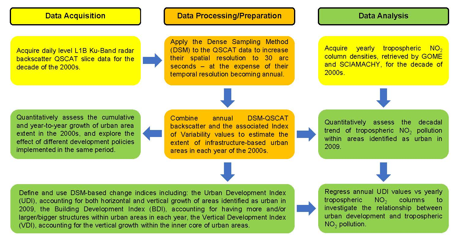
2. Study Area
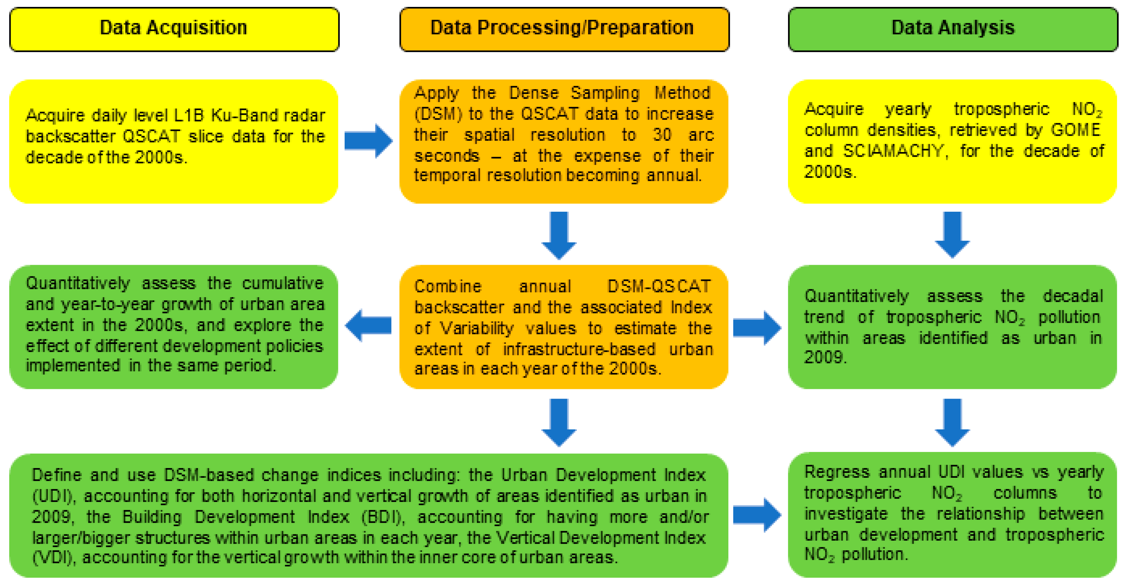
3. Materials and Methods
3.1. QSCAT Data and Dense Sampling Method for Urban Observations
3.2. Tropospheric NO2 Columns
4. Results and Discussion
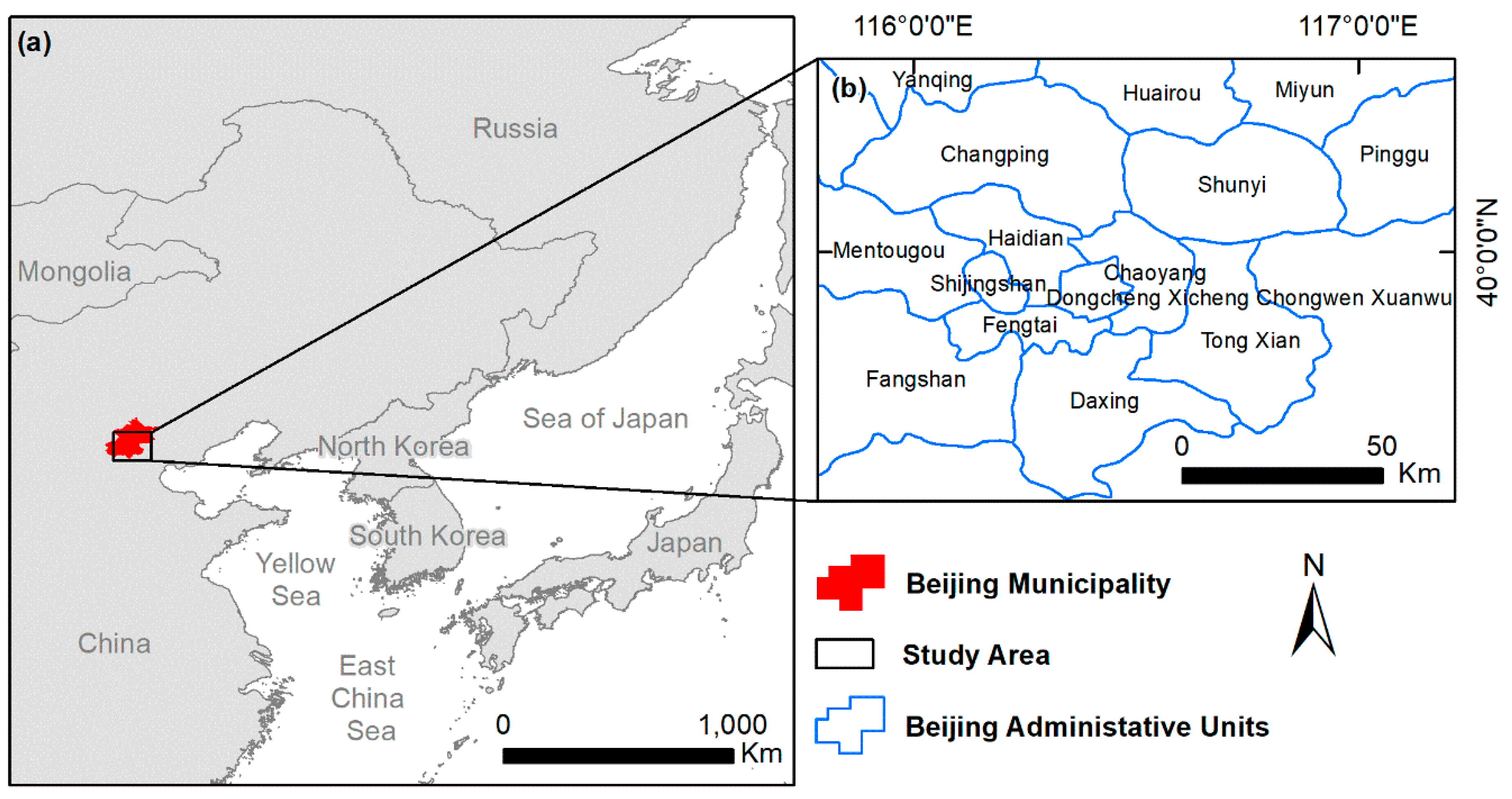
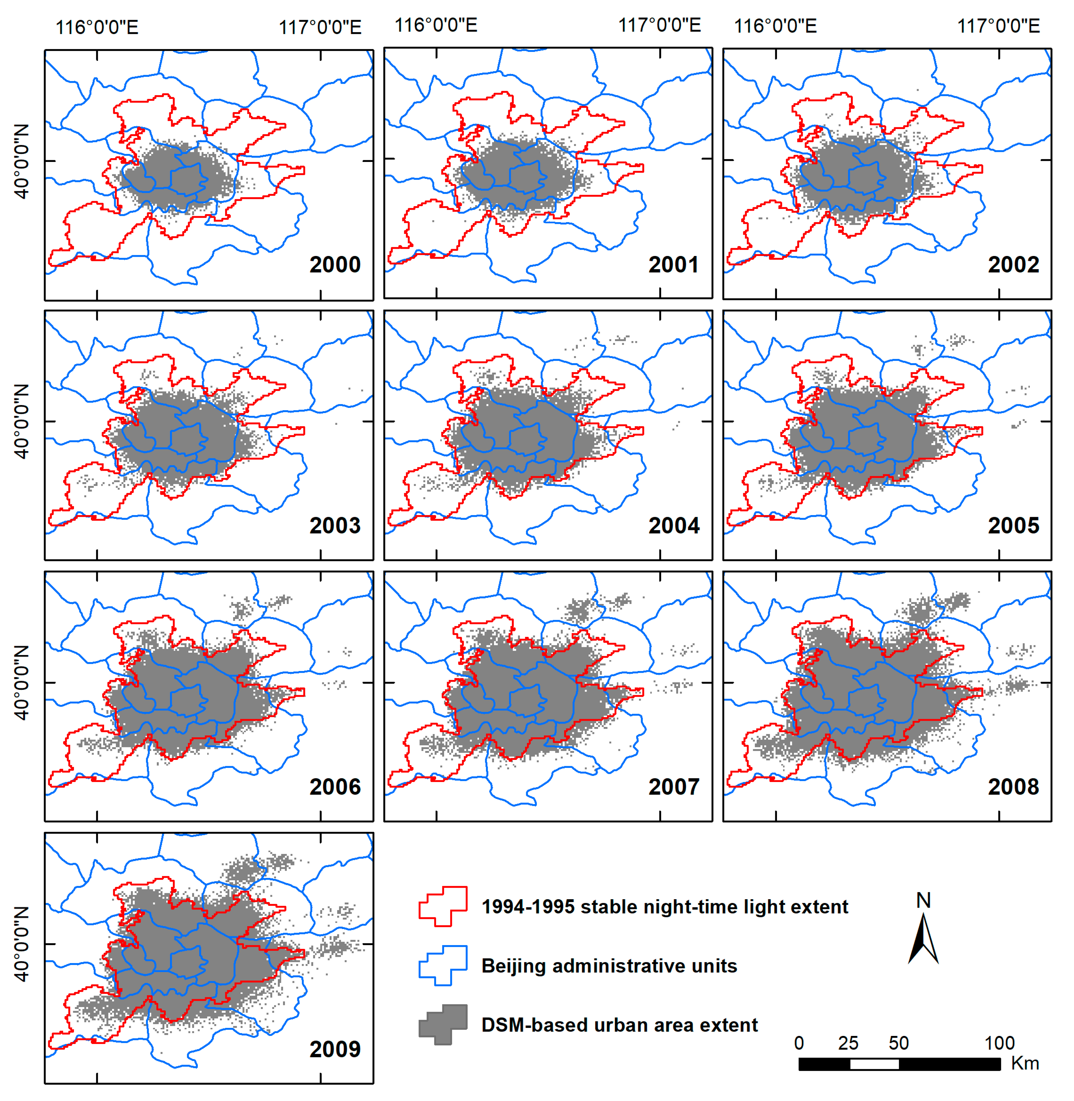
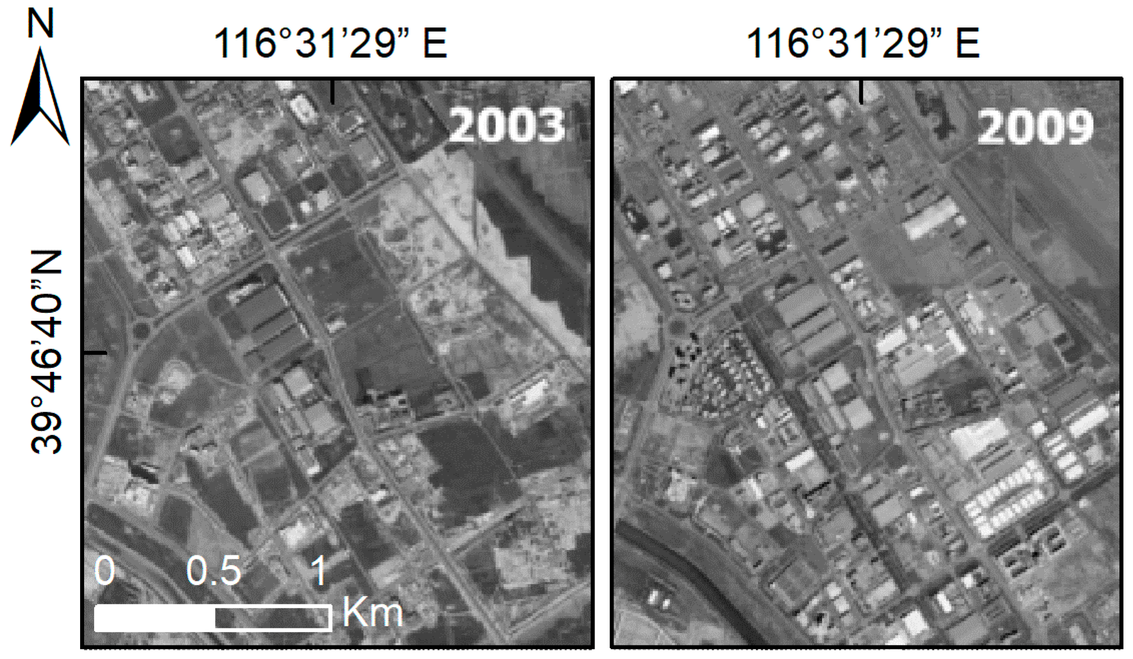
4.1. Beijing Urban Extent
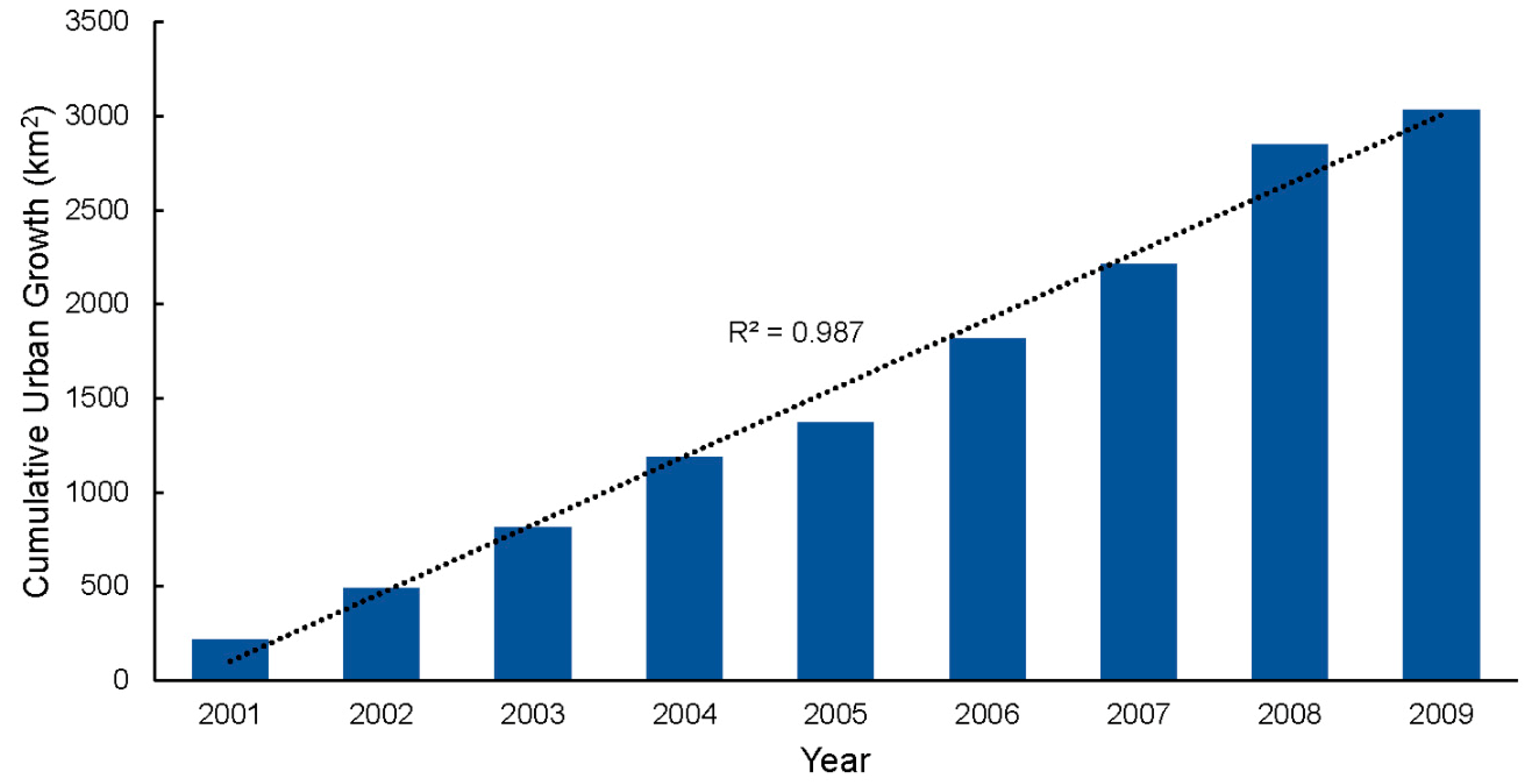
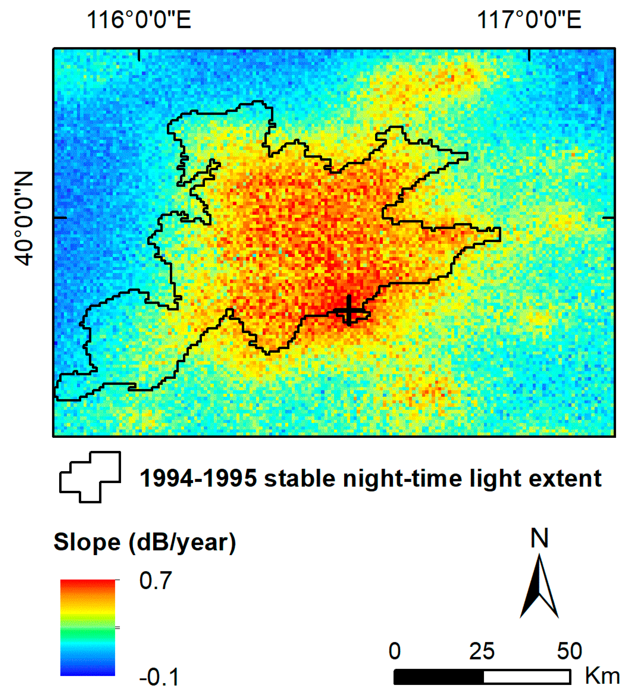
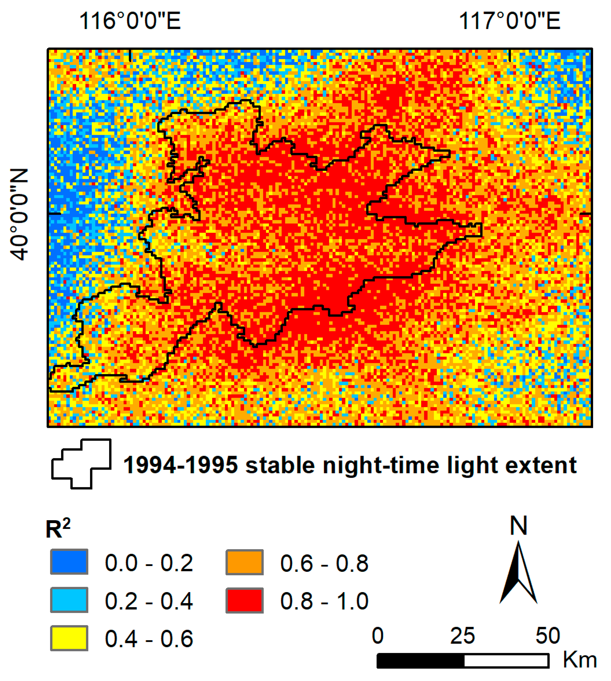
4.2. DSM-Based Change Indices
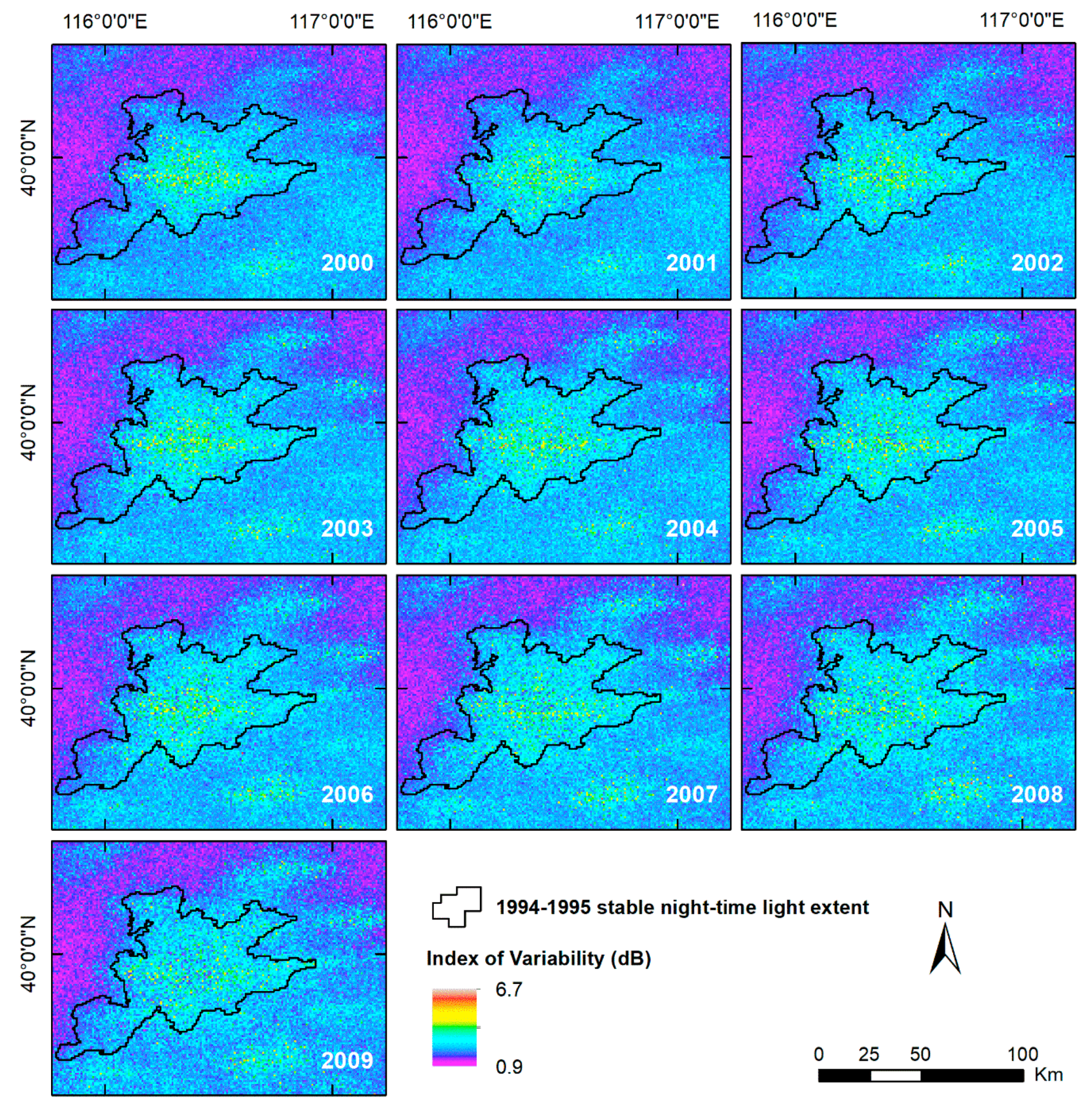
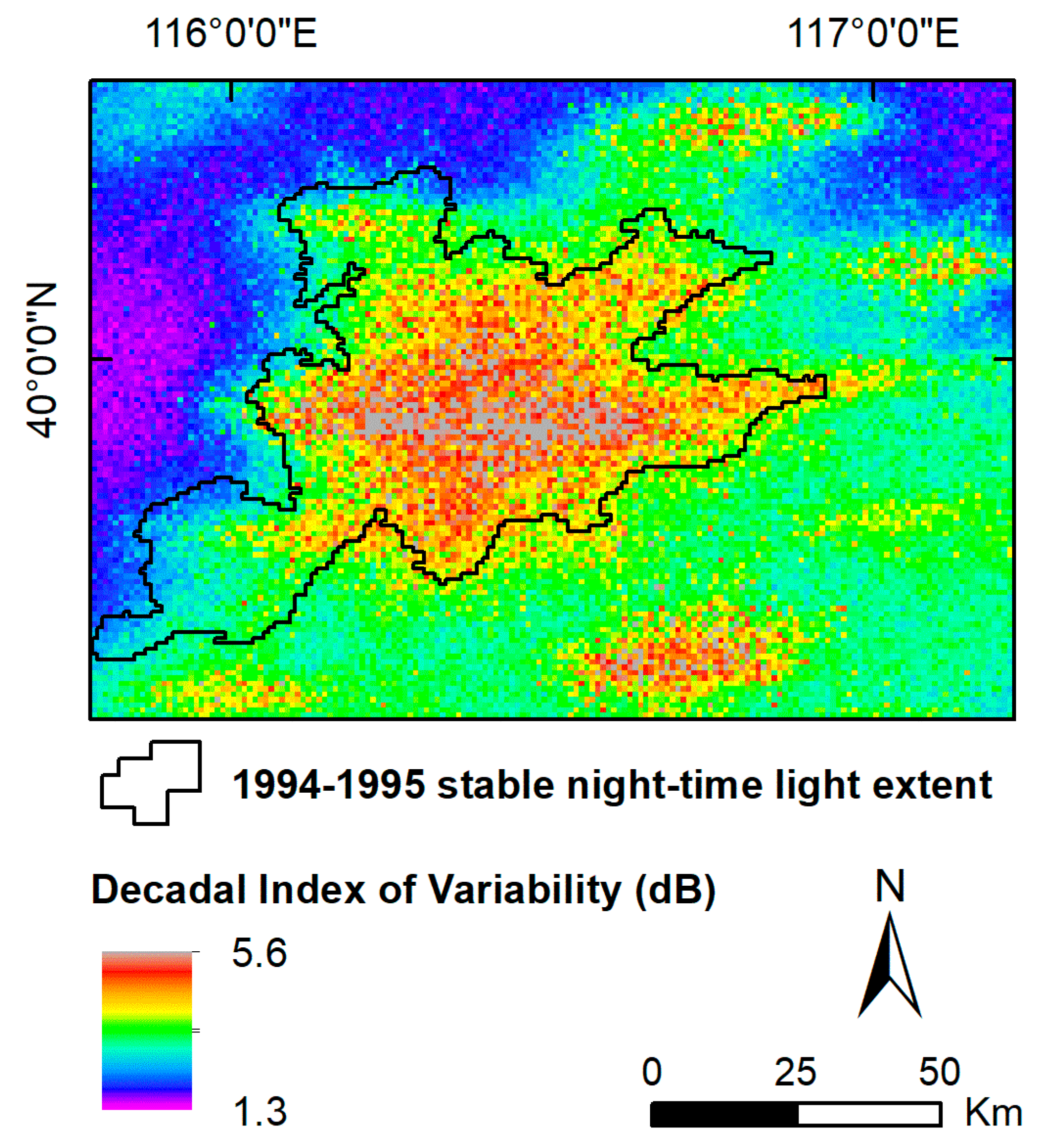
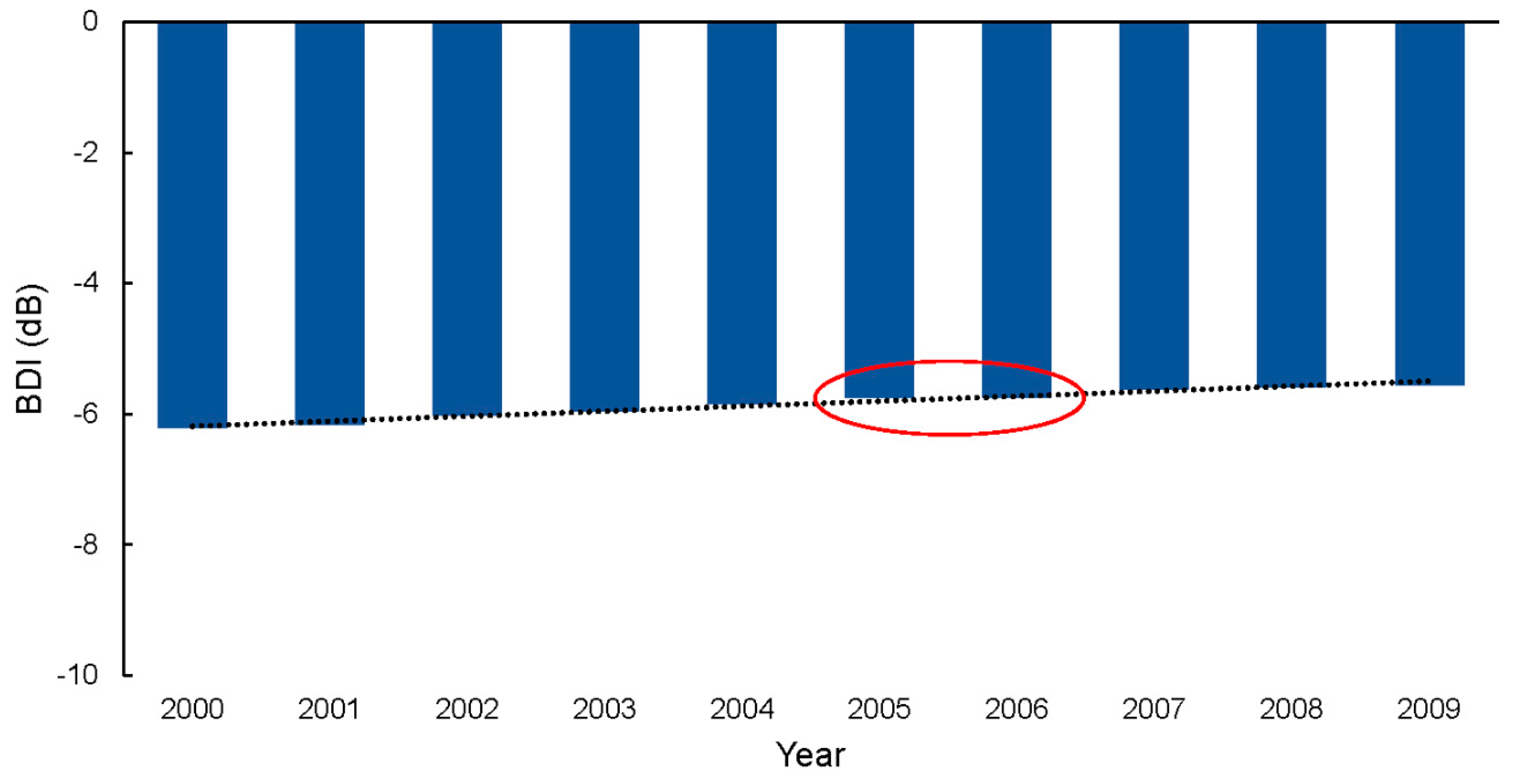
4.2.1. Surface Change Indices
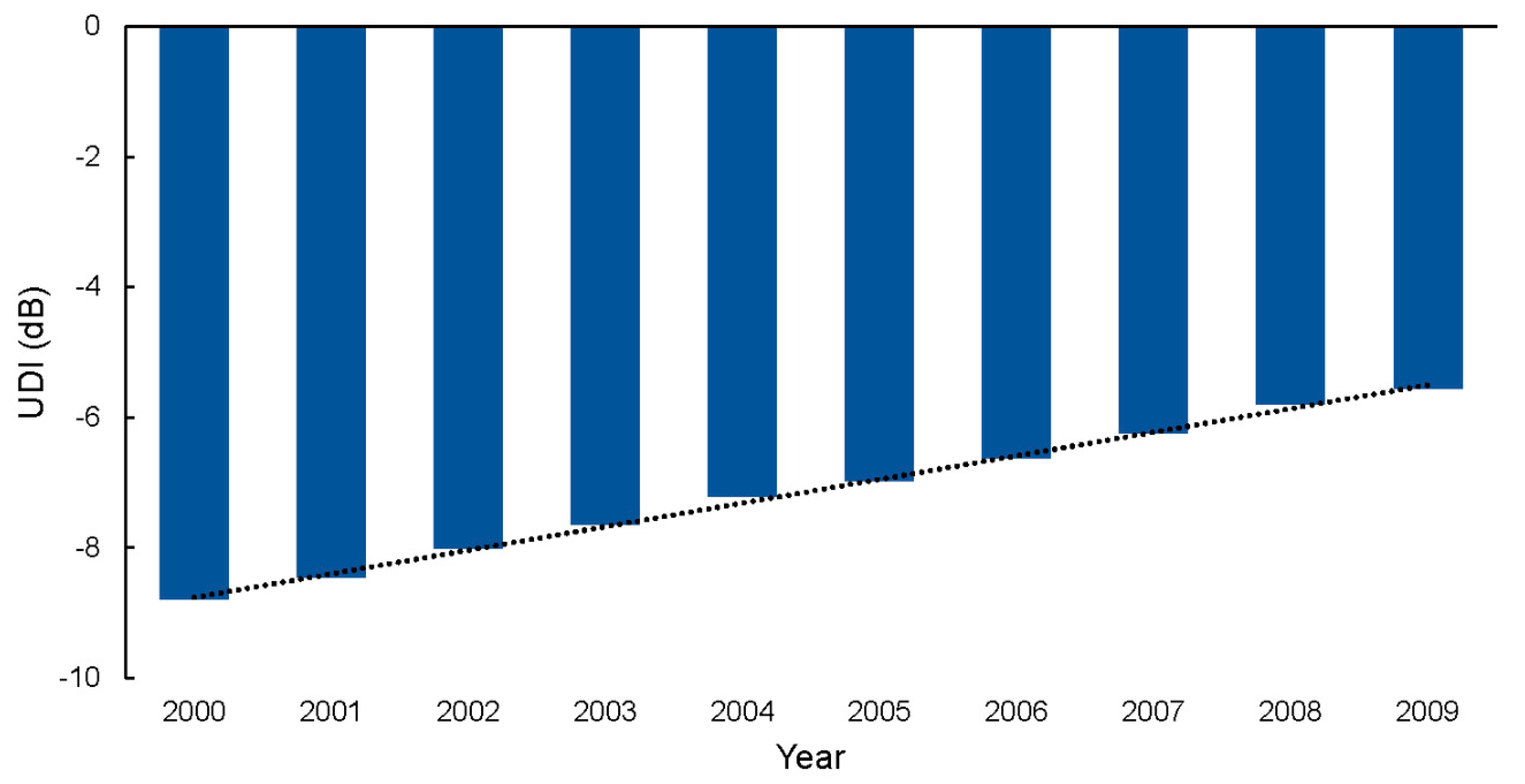
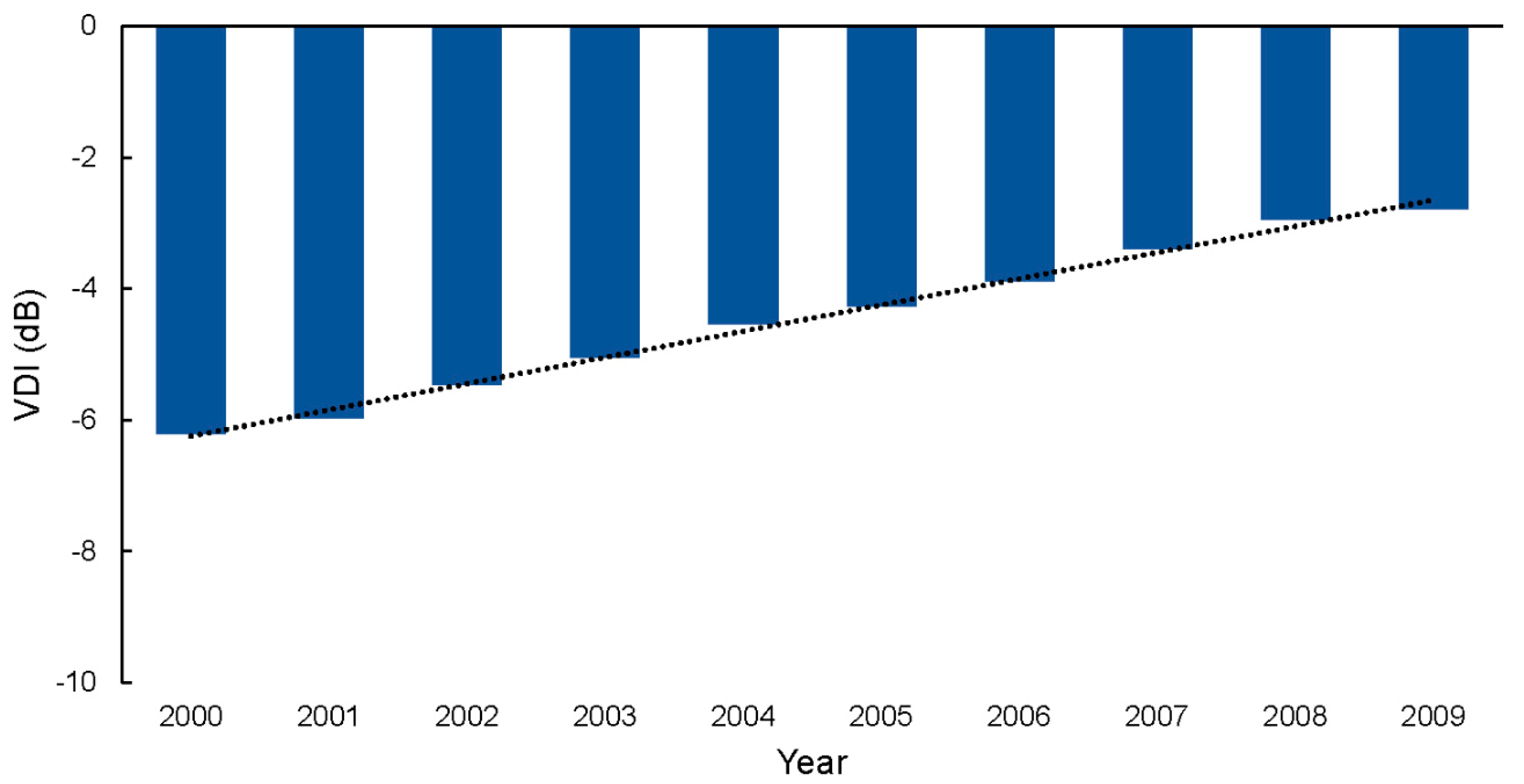
4.2.2. Development Indices
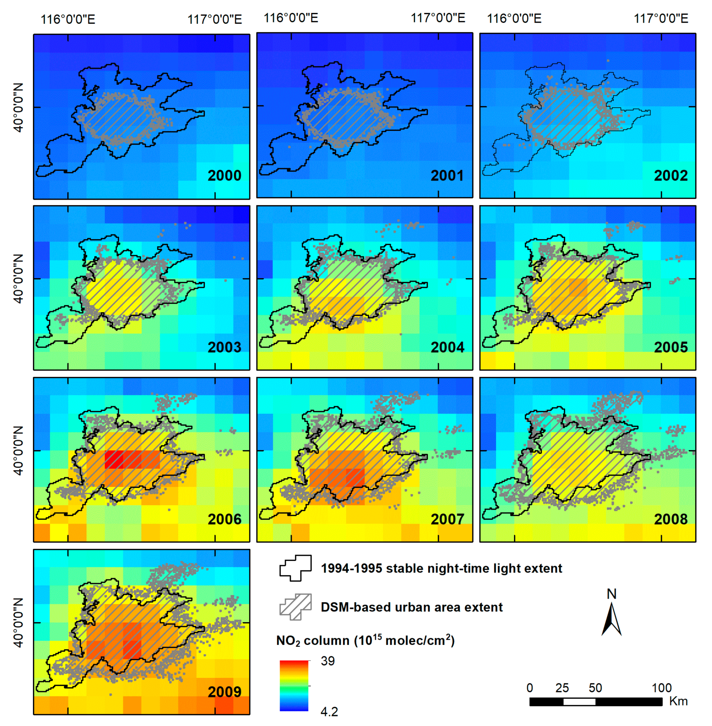
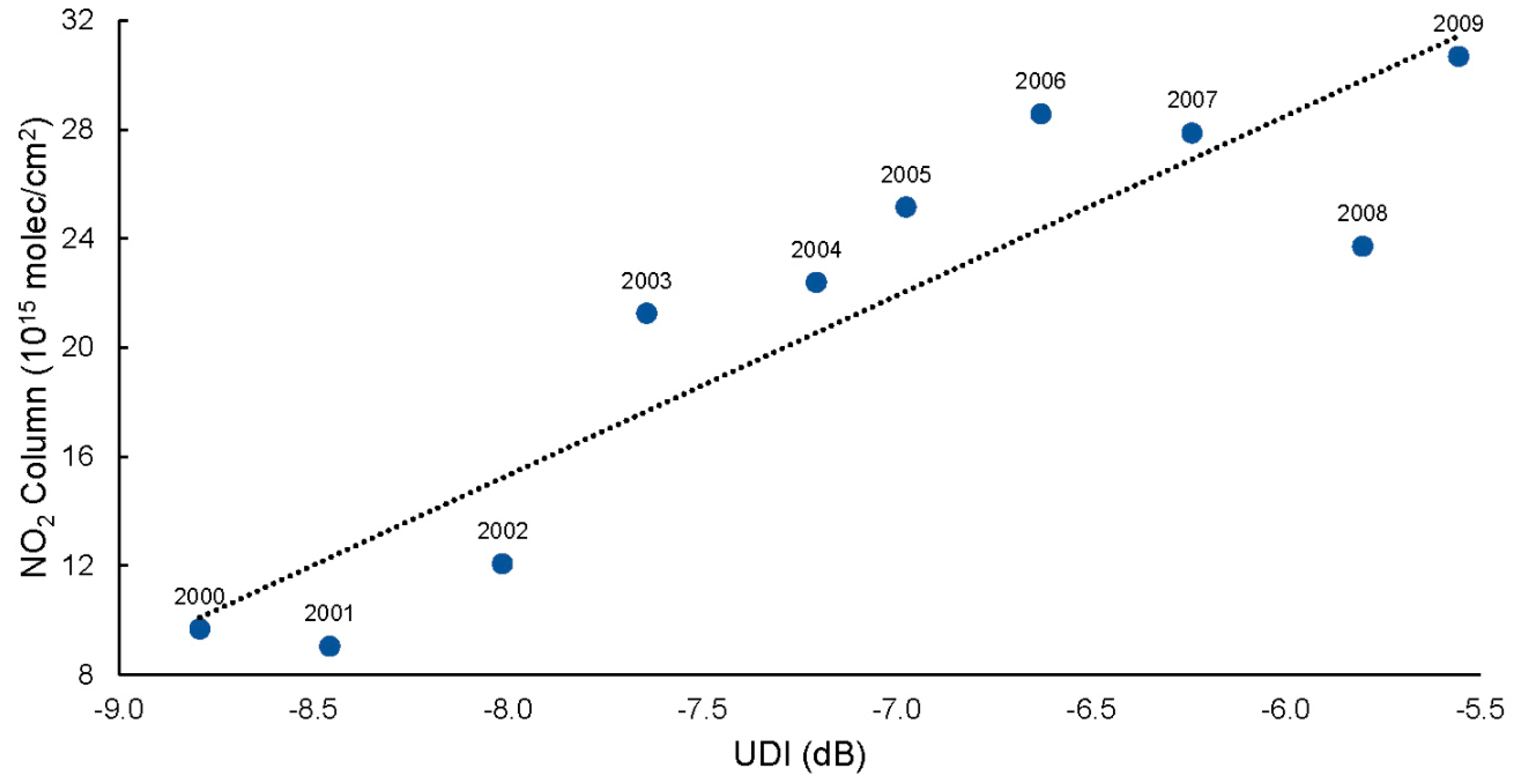
4.3. Beijing NO2 Pollution
5. Conclusions
Supplementary Materials
Author Contributions
Funding
Acknowledgments
Conflicts of Interest
References
- IPCC WGII and WGIII. In Proceedings of the Joint Expert Meeting of IPCC WGII and WGIII on Human Settlement, Water, Energy and Transport Infrastructure—Mitigation and Adaptation Strategies, Calcutta, India, 22–24 March 2011.
- Pachauri, R.K.; Allen, M.R.; Barros, V.R.; Broome, J.; Cramer, W.; Christ, R.; Church, J.A.; Clarke, L.; Dahe, Q.; Dasgupta, P.; et al. Climate Change 2014: Synthesis Report. Contribution of Working Groups I, II and III to the Fifth Assessment Report of the Intergovernmental Panel on Climate Change; IPCC: Geneva, Switzerland, 2014; p. 151. [Google Scholar]
- Chaussard, E.; Amelung, F.; Abidin, H.; Hong, S.H. Sinking cities in Indonesia: ALOS PALSAR detects rapid subsidence due to groundwater and gas extraction. Remote Sens. Environ. 2013, 128, 150–161. [Google Scholar] [CrossRef]
- Güneralp, B.; Güneralp, İ.; Liu, Y. Changing global patterns of urban exposure to flood and drought hazards. Glob. Environ. Chang. 2015, 31, 217–225. [Google Scholar] [CrossRef]
- IPCC. Managing the Risks of Extreme Events and Disasters to Advance Climate Change Adaptation. A Special Report of Working Groups I and II of the Intergovernmental Panel on Climate Change; Cambridge University Press: Cambridge, UK, 2012; p. 582. [Google Scholar]
- Geng, G.; Zhang, Q.; Martin, R.V.; van Donkelaar, A.; Huo, H.; Che, H.; Lin, J.; He, K. Estimating long-term PM 2.5 concentrations in China using satellite-based aerosol optical depth and a chemical transport model. Remote Sens. Environ. 2015, 166, 262–270. [Google Scholar] [CrossRef]
- Streets, D.G.; Fu, J.S.; Jang, C.J.; Hao, J.; He, K.; Tang, X.; Zhang, Y.; Wang, Z.; Li, Z.; Zhang, Q.; et al. Air quality during the 2008 Beijing Olympic games. Atmos. Environ. 2007, 41, 480–492. [Google Scholar] [CrossRef]
- Han, Z.; Ueda, H.; Matsuda, K. Model study of the impact of biogenic emission on regional ozone and the effectiveness of emission reduction scenarios over eastern China. Tellus B 2005, 57, 12–27. [Google Scholar] [CrossRef]
- National Intelligence Council (NIC). Global Trends 2030: Alternative Worlds; National Intelligence Council: Washington, DC, USA, 2012; p. 136.
- Han, H.Y.; Lai, S.K.; Dang, A.R.; Tan, Z.B.; Wu, C.F. Effectiveness of urban construction boundaries in Beijing: An assessment. J. Zhejiang Univ.-Sci. A 2009, 10, 1285–1295. [Google Scholar] [CrossRef]
- IPCC. Climate Change 2013: The Physical Science Basis. Contribution of Working Group I to the Fifth Assessment Report of the Intergovernmental Panel on Climate Change; Cambridge University Press: Cambridge, UK, 2013; p. 1535. [Google Scholar]
- Lin, C.; Li, Y.; Lau, A.K.; Deng, X.; Tim, K.T.; Fung, J.C.; Li, C.; Li, Z.; Lu, X.; Zhang, X.; et al. Estimation of long-term population exposure to PM 2.5 for dense urban areas using 1-km MODIS data. Remote Sens. Environ. 2016, 179, 13–22. [Google Scholar] [CrossRef] [Green Version]
- Jacobson, M.Z.; Nghiem, S.V.; Sorichetta, A. Short-term impacts of the megaurbanizations of New Delhi and Los Angeles between 2000 and 2009. J. Geophys. Res.-Atmos. 2019, 124, 35–56. [Google Scholar]
- Lin, C.H.; Tsai, P.H.; Lai, K.H.; Chen, J.Y. Cloud removal from multitemporal satellite images using information cloning. IEEE Trans. Geosci. Remote Sens. 2013, 51, 232–241. [Google Scholar] [CrossRef]
- Small, C. A global analysis of urban reflectance. Int. J. Remote Sens. 2005, 26, 661–681. [Google Scholar] [CrossRef]
- Li, C.C.; Wang, J.; Wang, L.; Hu, L.Y.; Gong, P. Comparison of classification algorithms and training sample sizes in urban land classification with Landsat Thematic Mapper imagery. Remote Sens. 2014, 6, 964–983. [Google Scholar] [CrossRef] [Green Version]
- Weng, Q.; Hu, X.; Liu, H. Estimating impervious surfaces using linear spectral mixture analysis with multitemporal ASTER images. Int. J. Remote Sens. 2009, 30, 4807–4830. [Google Scholar] [CrossRef]
- Small, C. High spatial resolution spectral mixture analysis of urban reflectance. Remote Sens. Environ. 2003, 88, 170–186. [Google Scholar] [CrossRef]
- Nghiem, S.V.; Balk, D.; Rodriguez, E.; Neumann, G.; Sorichetta, A.; Small, C.; Elvidge, C.D. Observations of urban and suburban environments with global satellite scatterometer data. ISPRS J. Photogramm. 2009, 64, 367–380. [Google Scholar] [CrossRef]
- Elvidge, C.D.; Imhoff, M.L.; Baugh, K.E.; Hobson, V.R.; Nelson, I.; Safran, J.; Dietz, J.B.; Tuttle, B.T. Night-time lights of the world: 1994–1995. ISPRS J. Photogramm. 2001, 56, 81–99. [Google Scholar] [CrossRef]
- Nghiem, S.V.; Sorichetta, A.; Elvidge, C.D.; Small, C.; Balk, D.; Deichmann, U.; Neumann, G. Urban Environments, Beijing Case Study. In Encyclopedia of Remote Sensing; Njoku, E.G., Ed.; Encyclopedia of Earth Sciences Series; Springer: New York, NY, USA, 2014; pp. 869–878. [Google Scholar]
- Small, C.; Pozzi, F.; Elvidge, C.D. Spatial analysis of global urban extent from DMSP-OLS night lights. Remote Sens. Environ. 2005, 96, 277–291. [Google Scholar] [CrossRef]
- Dell’Acqua, F. The role of SAR sensors. In Global Mapping of Human Settlement: Experiences, Datasets, and Prospects; Gamba, P., Herold, M., Eds.; CRC Press: Boca Raton, FL, USA, 2009; pp. 309–319. [Google Scholar]
- Farr, T.G.; Rosen, P.A.; Caro, E.; Crippen, R.; Duren, R.; Hensley, S.; Kobrick, M.; Paller, M.; Rodriguez, E.; Roth, L.; et al. The shuttle radar topography mission. Rev. Geophys. 2007, 45. [Google Scholar] [CrossRef] [Green Version]
- Esch, T.; Taubenböck, H.; Roth, A.; Heldens, W.; Felbier, A.; Thiel, M.; Schmidt, M.; Müller, A.; Dech, S. TanDEM-X mission—New perspectives for the inventory and monitoring of global settlement patterns. J. Appl. Remote Sens. 2012, 6, 061702. [Google Scholar] [CrossRef]
- Shahzad, M.; Maurer, M.; Fraundorfer, F.; Wang, Y.; Zhu, X.X. Buildings detection in VHR SAR images using fully convolution neural networks. IEEE Trans. Geosci. Remote Sens. 2019, 57, 1100–1116. [Google Scholar] [CrossRef] [Green Version]
- Mathews, A.J.; Frazier, A.E.; Nghiem, S.V.; Neumann, G.; Zhao, Y. Satellite scatterometer estimation of urban built-up volume: Validation with airborne lidar data. Int. J. Appl. Earth Obs. Geoinf. 2019, 77, 100–107. [Google Scholar] [CrossRef]
- Lungu, T.; Callahan, P.S.; Dunbar, S.; Weiss, B.; Stiles, B.; Huddleston, J.; Shirtcliffe, G.; Perry, K.L.; Hsu, C.; Mears, C.; et al. QuikSCAT Science Data Product User’s Manual; Version 3.0, D-18053-Rev A; Jet Propulsion Laboratory, California Institute of Technology: Pasadena, CA, USA, 2006.
- Burrows, J.P.; Weber, M.; Buchwitz, M.; Rozanov, V.; Ladstätter-Weißenmayer, A.; Richter, A.; DeBeek, R.; Hoogen, R.; Bramstedt, K.; Eichmann, K.U.; et al. The global ozone monitoring experiment (GOME): Mission concept and first scientific results. J. Atmos. Sci. 1999, 56, 151–175. [Google Scholar] [CrossRef]
- Richter, A.; Burrows, J.P. Tropospheric NO2 from GOME measurements. Adv. Space Res. 2002, 29, 1673–1683. [Google Scholar] [CrossRef]
- Bovensmann, H.; Burrows, J.P.; Buchwitz, M.; Frerick, J.; Noël, S.; Rozanov, V.V.; Chance, K.V.; Goede, A.P.H. SCIAMACHY: Mission objectives and measurement modes. J. Atmos. Sci. 1999, 56, 127–150. [Google Scholar] [CrossRef] [Green Version]
- Wang, Y.; Ren, X.; Ji, D.; Zhang, J.; Sun, J.; Wu, F. Characterization of volatile organic compounds in the urban area of Beijing from 2000 to 2007. J. Environ. Sci. 2012, 24, 95–101. [Google Scholar] [CrossRef]
- Long, Y.; Han, H.; Lai, S.K.; Mao, Q. Urban growth boundaries of the Beijing Metropolitan Area: Comparison of simulation and artwork. Cities 2013, 31, 337–348. [Google Scholar] [CrossRef]
- GADM Maps and Data. Available online: https://gadm.org/ (accessed on 3 October 2019).
- Long, Y.; Mao, Q.; Dang, A. Beijing urban development model: Urban growth analysis and simulation. Tsinghua Sci. Technol. 2009, 14, 782–794. [Google Scholar] [CrossRef]
- Wikipedia—Beijing. Available online: https://en.wikipedia.org/wiki/Beijing (accessed on 2 November 2019).
- Sun, Y.; Wang, L.; Wang, Y.; Quan, L.; Zirui, L. In situ measurements of SO2, NOx, NOy, and O3 in Beijing, China during August 2008. Sci. Total. Environ. 2011, 409, 933–940. [Google Scholar] [CrossRef]
- Hatakeyama, S.; Takami, A.; Wang, W.; Tang, D. Aerial observation of air pollutants and aerosols over Bo Hai, China. Atmos. Environ. 2005, 39, 5893–5898. [Google Scholar] [CrossRef]
- Tsai, W.Y.; Nghiem, S.V.; Huddleston, J.N.; Spencer, M.W.; Stiles, B.W.; West, R.D. Polarimetric scatterometry: A promising technique for improving ocean surface wind measurements from space. IEEE Trans. Geosci. Remote Sens. 2000, 38, 1903–1921. [Google Scholar] [CrossRef]
- Nghiem, S.V.; Leshkevich, G.A.; Stiles, B.W. Wind fields over the Great Lakes measured by the Sea Winds scatterometer on the QuikSCAT satellite. J. Great Lakes Res. 2004, 30, 148–165. [Google Scholar] [CrossRef]
- Stevenazzi, S.; Masetti, M.; Nghiem, S.V.; Sorichetta, A. Groundwater vulnerability maps derived from time dependent method using satellite scatterometer data. Hydrogeol. J. 2015, 23, 631–647. [Google Scholar] [CrossRef]
- Stevenazzi, S.; Bonfanti, M.; Masetti, M.; Nghiem, S.V.; Sorichetta, A. A versatile method for groundwater vulnerability projections in future scenarios. J. Environ. Manag. 2017, 187, 365–374. [Google Scholar] [CrossRef] [PubMed]
- Jacobson, M.Z.; Nghiem, S.V.; Sorichetta, A.; Whitney, N.S. Ring of impact from the mega-urbanization of Beijing between 2000 and 2009. J. Geophys. Res.-Atmos. 2015, 120, 5740–5756. [Google Scholar] [CrossRef]
- Masetti, M.; Nghiem, S.V.; Sorichetta, A.; Stevenazzi, S.; Fabbri, P.; Pola, M.; Filippini, M.; Brakenridge, G.R. Urbanization affects air and water in Italy’s Po Plain. Eos 2015, 96, 13–16. [Google Scholar] [CrossRef]
- Zhang, Q.; Pandey, B.; Seto, K.C.A. Robust Method to Generate a Consistent Time Series From DMSP/OLS Nighttime Light Data. IEEE Trans. Geosci. Remote Sens. 2016, 54, 5821–5831. [Google Scholar] [CrossRef]
- Nguyen, L.H.; Nghiem, S.V.; Henebry, G.M. Expansion of major urban areas in the US Great Plains from 2000 to 2009 using satellite scatterometer data. Remote Sens. Environ. 2018, 204, 524–533. [Google Scholar] [CrossRef]
- Welcome at the IUP-Bremen DOAS Group. Available online: http://www.doas-bremen.de/index.html (accessed on 3 October 2019).
- Richter, A.; Burrows, J.P.; Nüß, H.; Granier, C.; Niemeier, U. Increase in tropospheric nitrogen dioxide over China observed from space. Nature 2005, 437, 129–132. [Google Scholar] [CrossRef]
- Zhang, Q.; Streets, D.G.; He, K.; Wang, Y.; Richter, A.; Burrows, J.P.; Uno, I.; Jang, C.J.; Chen, D.; Yao, Z.; et al. NOx emission trends for China, 1995–2004: The view from the ground and the view from space. J. Geophys. Res.-Atmos. 2007, 112. [Google Scholar] [CrossRef] [Green Version]
- Huang, J.; Zhou, C.; Lee, X.; Bao, Y.; Zhao, X.; Fung, J.; Richter, A.; Liu, X.; Zheng, Y. The effects of rapid urbanization on the levels in tropospheric nitrogen dioxide and ozone over East China. Atmos. Environ. 2013, 77, 558–567. [Google Scholar] [CrossRef]
- Hilboll, A.; Richter, A.; Burrows, J.P. NO2 pollution over India observed from space—The impact of rapid economic growth, and a recent decline. Atmos. Chem. Phys. Discuss. 2017. [Google Scholar] [CrossRef] [Green Version]
- Petritoli, A.; Bonasoni, P.; Giovanelli, G.; Ravegnani, F.; Kostadinov, I.; Bortoli, D.; Weiss, A.; Schaub, D.; Richter, A.; Fortezza, F. First comparison between ground-based and satellite-borne measurements of tropospheric nitrogen dioxide in the Po basin. J. Geophys. Res.-Atmos. 2004, 109. [Google Scholar] [CrossRef] [Green Version]
- Nghiem, S.V.; Tsai, W.Y. Global snow cover monitoring with spaceborne K/sub u/-band scatterometer. IEEE Trans. Geosci. Remote Sens. 2001, 39, 2118–2134. [Google Scholar] [CrossRef] [Green Version]
- Santini, M.; Taramelli, A.; Sorichetta, A. ASPHAA: A GIS-based algorithm to calculate cell area on a latitude-longitude (geographic) regular grid. Trans. GIS 2010, 14, 351–377. [Google Scholar] [CrossRef]
- Xie, Y.; Fang, C.; Lin, G.; Gong, H.; Qiao, B. Tempo-spatial patterns of land use changes and urban development in globalizing China: A study of Beijing. Sensors 2007, 7, 2881–2906. [Google Scholar] [CrossRef] [Green Version]
- Ebeijing—Land Area and Utilization 2007. Available online: http://www.ebeijing.gov.cn/feature_2/Statistics/GeneralSuvey/t1067970.htm (accessed on 3 October 2019).
- Wikipedia—Geography of Beijing. Available online: http://en.wikipedia.org/wiki/Geography_of_Beijing (accessed on 3 October 2019).
- Broudehoux, A.M. Spectacular Beijing: The conspicuous construction of an Olympic metropolis. J. Urban Aff. 2007, 29, 383–399. [Google Scholar] [CrossRef] [Green Version]
- Shenghe, L.; Prieler, S.; Xiubin, L. Spatial patterns of urban land use growth in Beijing. J. Geogr. Sci. 2002, 12, 266–274. [Google Scholar] [CrossRef]
- U.S. Environmental Protection Agency—Nitrogen Dioxide (NO2) Pollution. Available online: https://www.epa.gov/no2-pollution/basic-information-about-no2#Effects (accessed on 3 October 2019).
- Rich, D.Q.; Kipen, H.M.; Huang, W.; Wang, G.; Wang, Y.; Zhu, P.; Ohman-Strickland, P.; Hu, M.; Philipp, C.; Diehl, S.R.; et al. Association between changes in air pollution levels during the Beijing Olympics and biomarkers of inflammation and thrombosis in healthy young adults. JAMA 2012, 307, 2068–2078. [Google Scholar] [CrossRef]
- Schleicher, N.; Norra, S.; Chen, Y.; Chai, F.; Wang, S. Efficiency of mitigation measures to reduce particulate air pollution—A case study during the Olympic Summer Games 2008 in Beijing, China. Sci. Total. Environ. 2012, 427, 146–158. [Google Scholar] [CrossRef]
- European Space Agency—Copernicus. Available online: http://www.esa.int/Our_Activities/Observing_the_Earth/Copernicus/Overview4 (accessed on 3 October 2019).
- NASA-ISRO SAR Mission (NISAR). Available online: http://nisar.jpl.nasa.gov/ (accessed on 3 October 2019).
- Schneider, A.; Friedl, M.A.; Potere, D. A new map of global urban extent from MODIS satellite data. Environ. Res. Lett. 2009, 4, 044003. [Google Scholar] [CrossRef] [Green Version]
- Zhou, Y.; Smith, S.J.; Zhao, K.; Imhoff, M.; Thomson, A.; Bond-Lamberty, B.; Asrar, G.R.; Zhang, X.; He, C.; Elvidge, C.D. A global map of urban extent from nightlights. Environ. Res. Lett. 2015, 10, 054011. [Google Scholar] [CrossRef]
- Pesaresi, M.; Ehrlich, D.; Ferri, S.; Florczyk, A.J.; Freire, S.; Halkia, M.; Julea, A.; Kemper, T.; Soille, P.; Syrris, V. Operating Procedure for the Production of the Global Human Settlement Layer from Landsat Data of the Epochs 1975, 1990, 2000, and 2014; Publications Office of the European Union: Luxembourg, 2016; pp. 1–62. [Google Scholar]


| Year | Surface of Urban Area Extent | Annual Growth (with Respect to the Previous Year) | ||
|---|---|---|---|---|
| No. of Grid Cells | km2 | km2 | % | |
| 2000 | 1676 | 1104.83 | ||
| 2001 | 2002 | 1319.74 | 214.9 | 19.5 |
| 2002 | 2423 | 1597.23 | 277.5 | 21.0 |
| 2003 | 2906 | 1915.55 | 318.3 | 19.9 |
| 2004 | 3477 | 2291.79 | 376.2 | 19.6 |
| 2005 | 3759 | 2477.53 | 185.7 | 8.1 |
| 2006 | 4432 | 2920.76 | 443.2 | 17.9 |
| 2007 | 5035 | 3317.93 | 397.2 | 13.6 |
| 2008 | 5999 | 3952.85 | 634.9 | 19.1 |
| 2009 | 6282 | 4139.33 | 186.5 | 4.7 |
© 2020 by the authors. Licensee MDPI, Basel, Switzerland. This article is an open access article distributed under the terms and conditions of the Creative Commons Attribution (CC BY) license (http://creativecommons.org/licenses/by/4.0/).
Share and Cite
Sorichetta, A.; Nghiem, S.V.; Masetti, M.; Linard, C.; Richter, A. Transformative Urban Changes of Beijing in the Decade of the 2000s. Remote Sens. 2020, 12, 652. https://doi.org/10.3390/rs12040652
Sorichetta A, Nghiem SV, Masetti M, Linard C, Richter A. Transformative Urban Changes of Beijing in the Decade of the 2000s. Remote Sensing. 2020; 12(4):652. https://doi.org/10.3390/rs12040652
Chicago/Turabian StyleSorichetta, Alessandro, Son V. Nghiem, Marco Masetti, Catherine Linard, and Andreas Richter. 2020. "Transformative Urban Changes of Beijing in the Decade of the 2000s" Remote Sensing 12, no. 4: 652. https://doi.org/10.3390/rs12040652