Joint Exploitation of SAR and GNSS for Atmospheric Phase Screens Retrieval Aimed at Numerical Weather Prediction Model Ingestion


Abstract
:
1. Introduction
2. Requirements for NWPM Ingestion, SAR Atmospheric Signal Characterization, and Orbit Requirements
2.1. Requirements for NWPM Ingestion
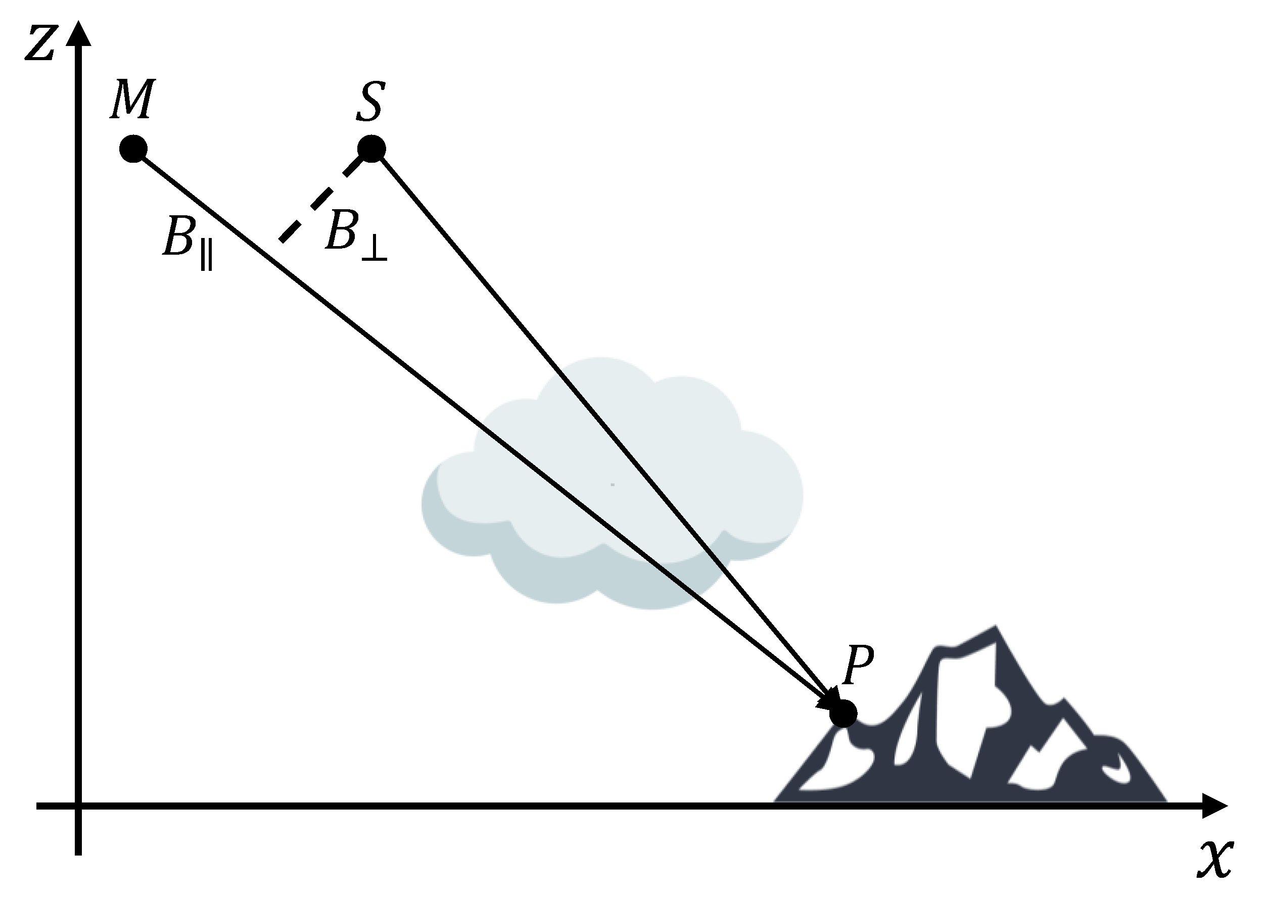
2.2. Atmospheric Contribution in SAR Images
- (1).
- can be removed easily from the interferometric phase by knowing the acquisition geometry and a Digital Elevation Model (DEM) of the scene.
- (2).
- (3).
- The phase of the target remains stable between the two acquisitions (.
2.3. Orbit Accuracy Requirements
3. Target Characterization
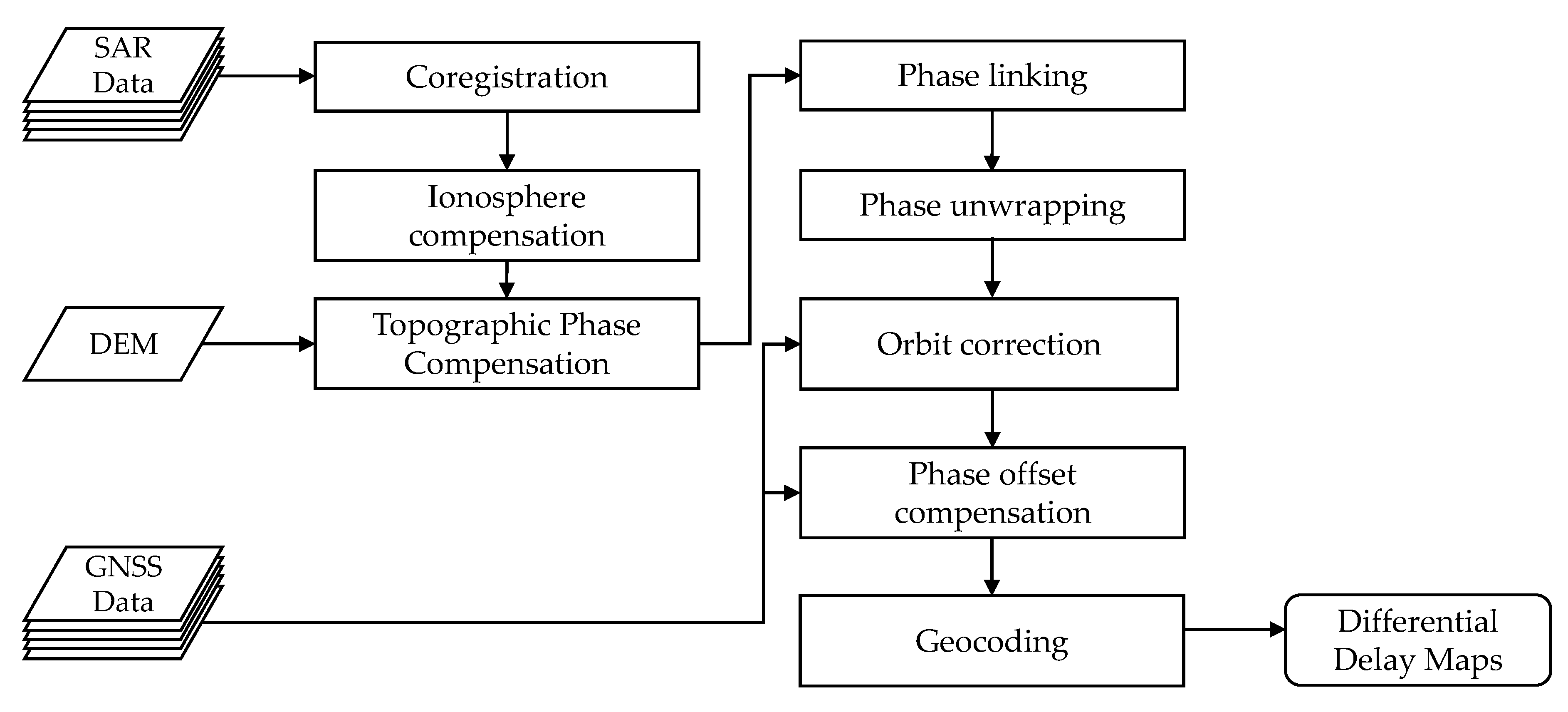
4. Processing Scheme
4.1. Coregistration and Ionospheric Phase Compensation
4.2. Topographic Phase Compensation
4.3. Phase Estimation via Phase Linking
- (1).
- The phase linking estimator just explained.
- (2).
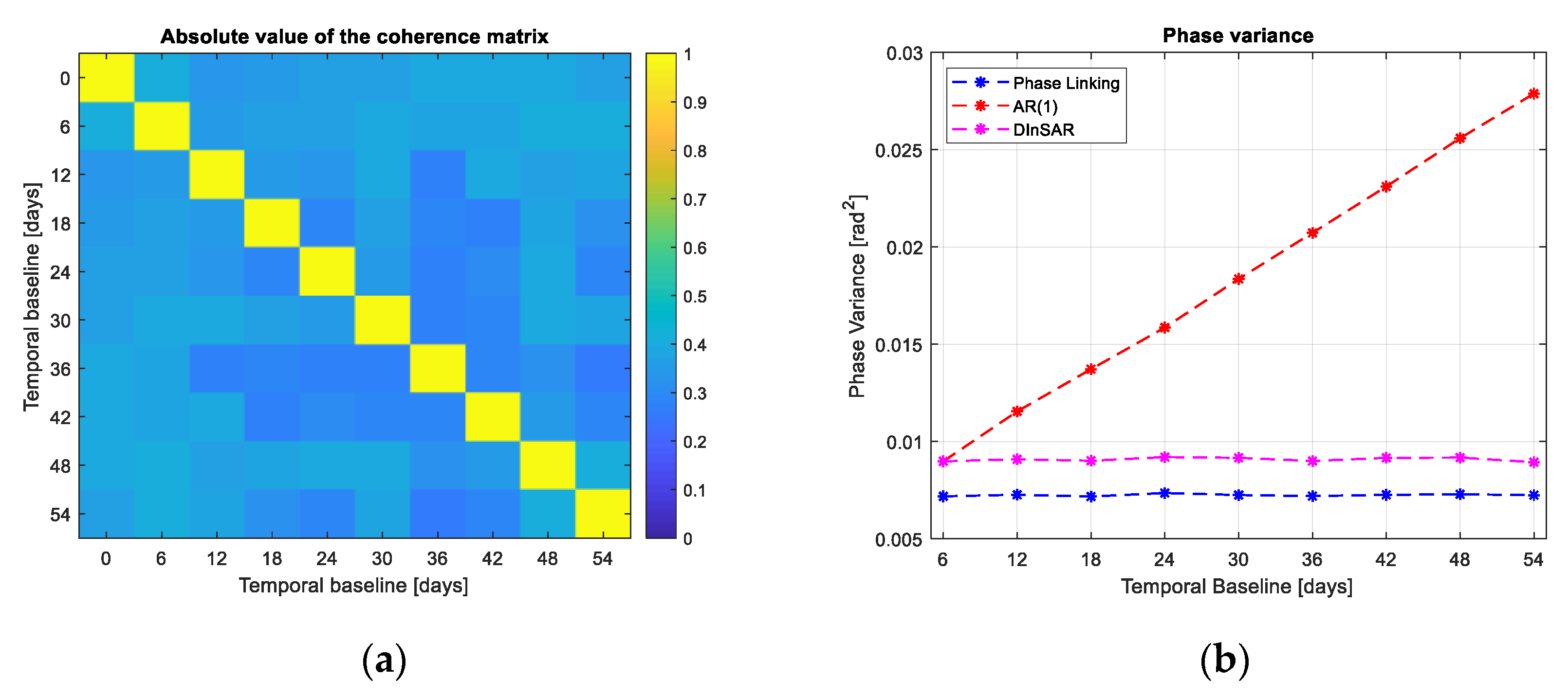
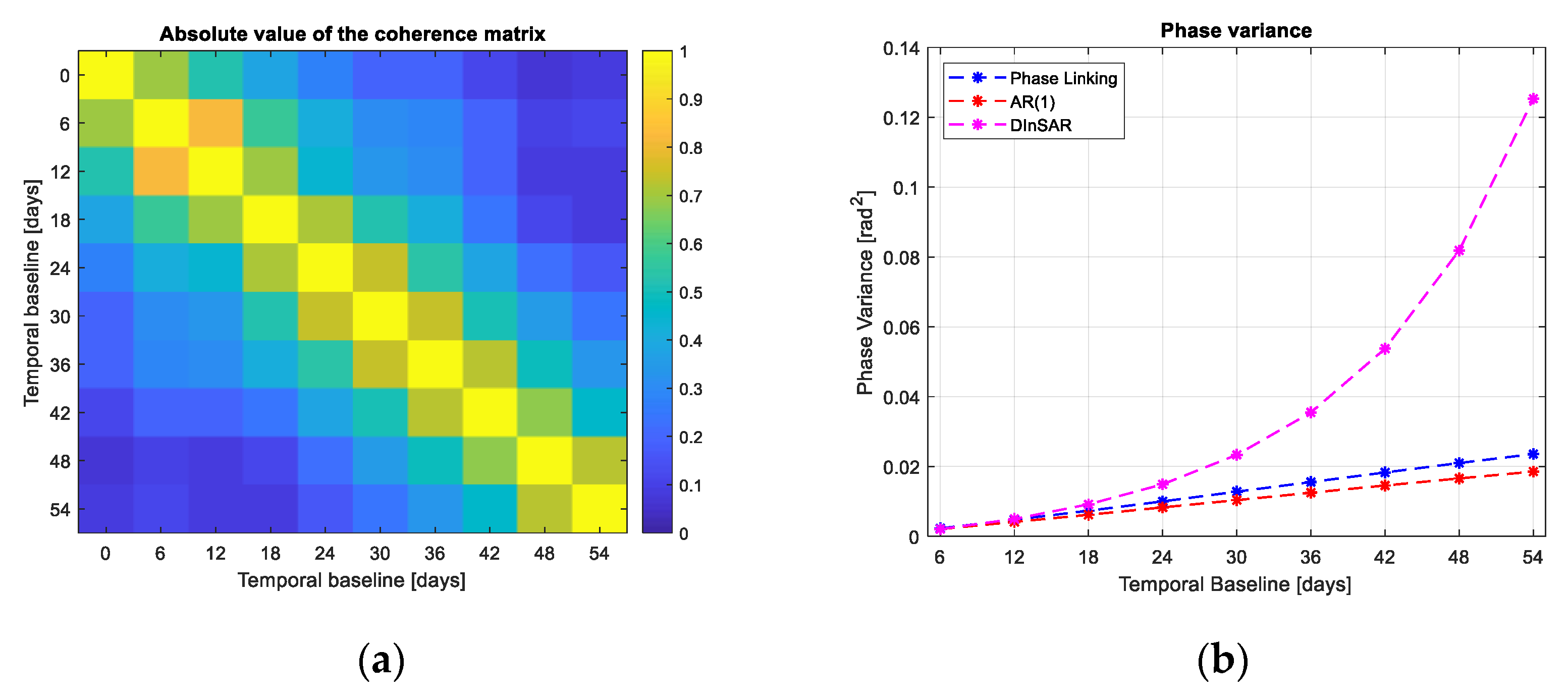
- The AR(1) estimator that consists in integrating the phases of interferograms formed using consecutive acquisitions:where is the complex element inside the sample coherence matrix at row a column . This method takes advantage of the high coherence of interferograms formed with consecutive acquisitions. It is also possible to show that, if in equation (7) we force , the AR(1) estimator is the exact estimator (in Maximum Likelihood sense).
4.4. Phase Linking for APS Estimation
- It reduces the effects of subsidences on the interferometric phase. The model of the interferometric phase in Equation (5) can present another term due to linear displacement in the line of sight direction that is equal to:where . In the presence of a normal subsidence rate in the order of 10 mm/year (i.e., not the one induced by an earthquake or a seismic event), if the stack is kept short (let us say eight images with a temporal extent of about 50 days), the error will be of less than 2 mm that is tolerable for our purposes.
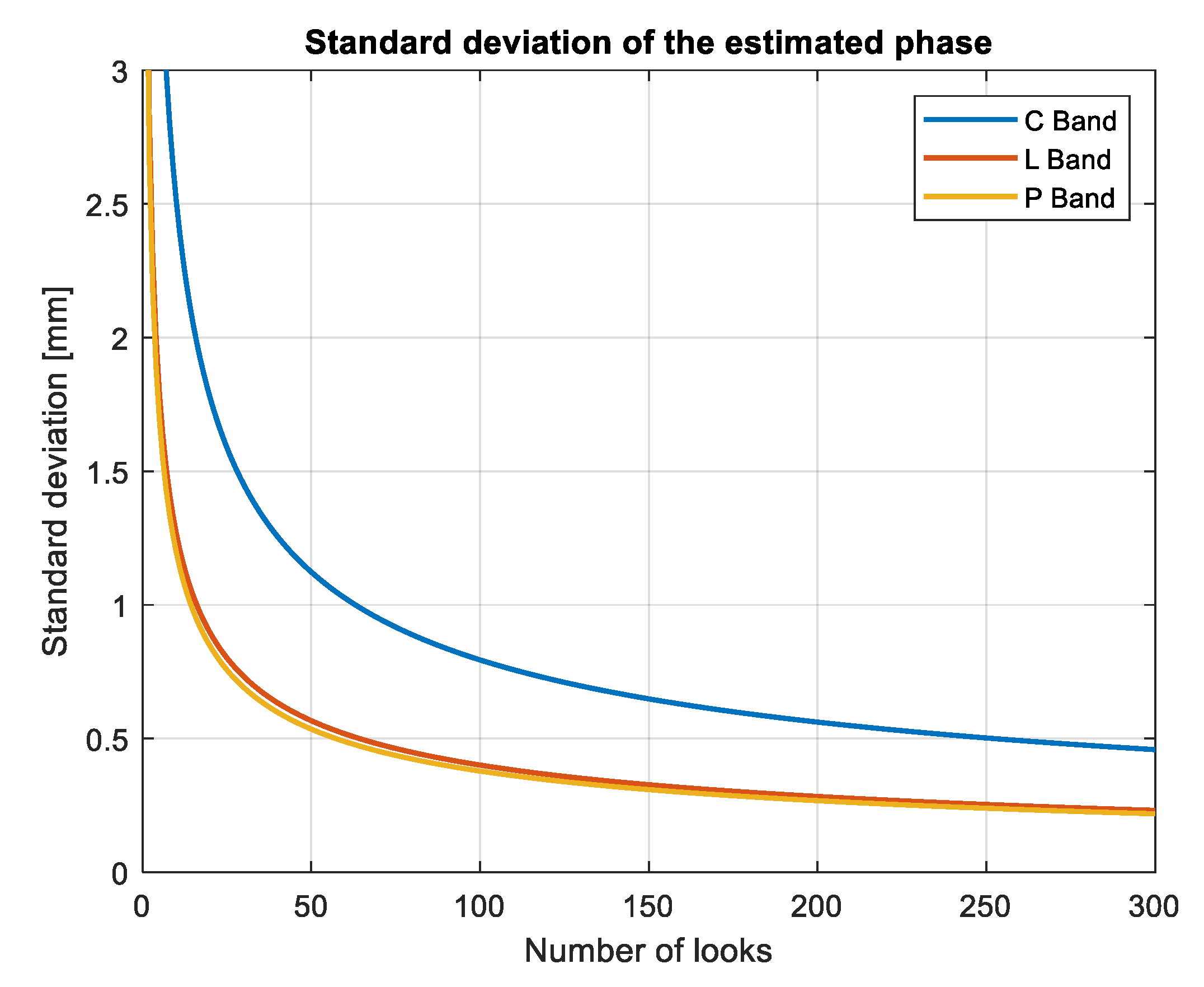
- Following the decorrelation model explained in Section 3, we can say that the stack temporal extent needs to take into consideration the average “life” of a distributed scatterer. With phase linking, we form all the possible interferograms with N images and from them, we estimate N-1 phases, if the coherence of the interferograms with very long temporal baseline is very low, they will bring noise into the final estimate. A solution is then to reduce the maximum temporal baseline by considering the decorrelation model. It is useful to remember that the decorrelation time depends on the wavelength used for the measure: In [18], Rocca made the example of 40 days in C-Band, but the reasoning can be easily extended in L or P Band where the average decorrelation time is much higher and thus a larger dataset can be used.
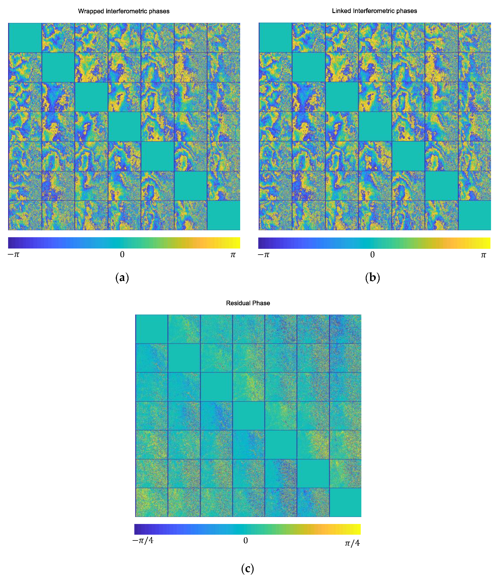
4.5. Phase Unwrapping
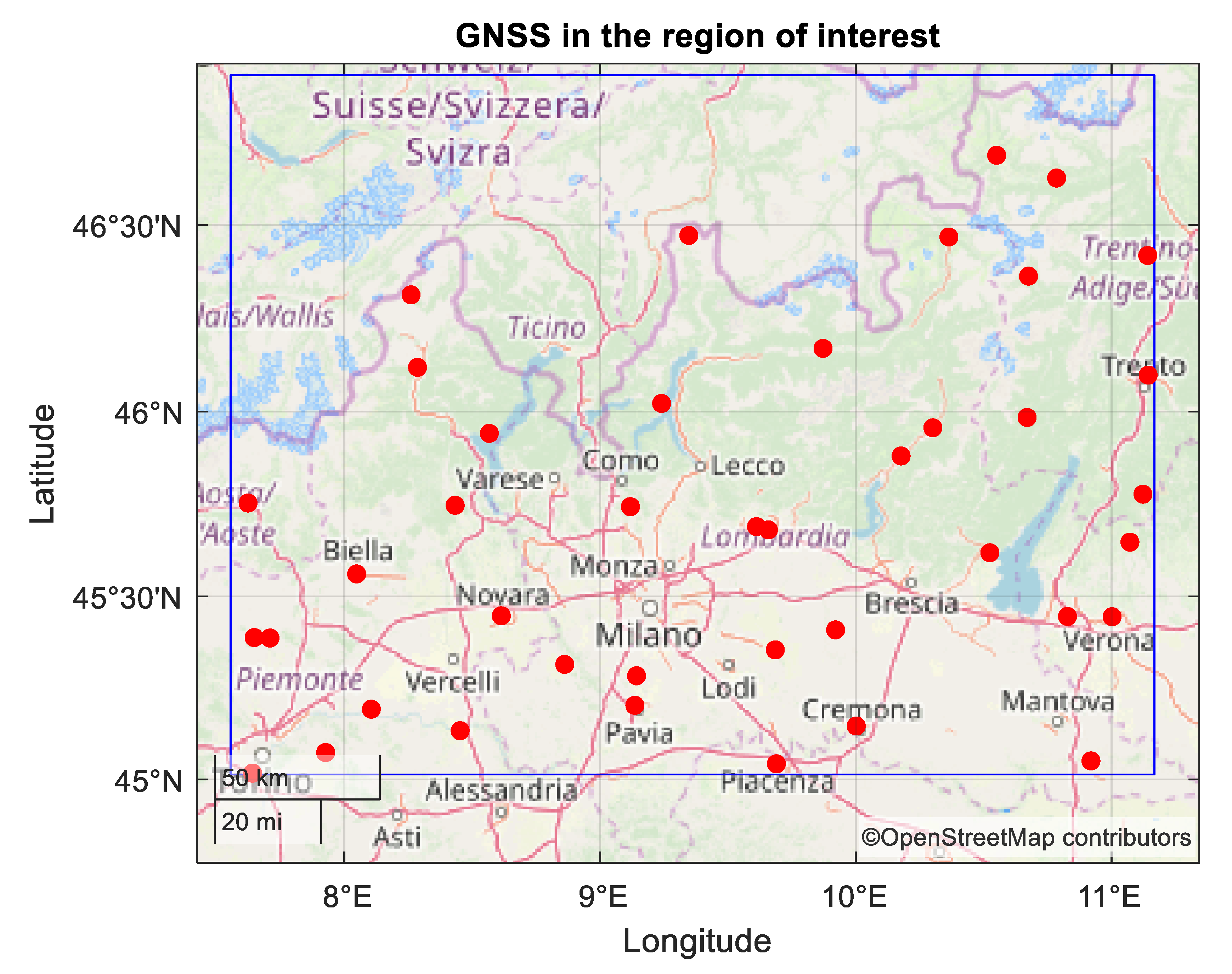
4.6. Orbit Correction: GNSS Processing and Integration
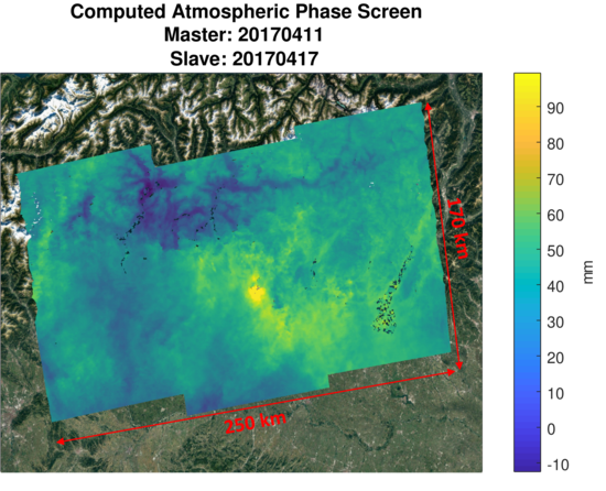
5. Case Study
5.1. Dataset
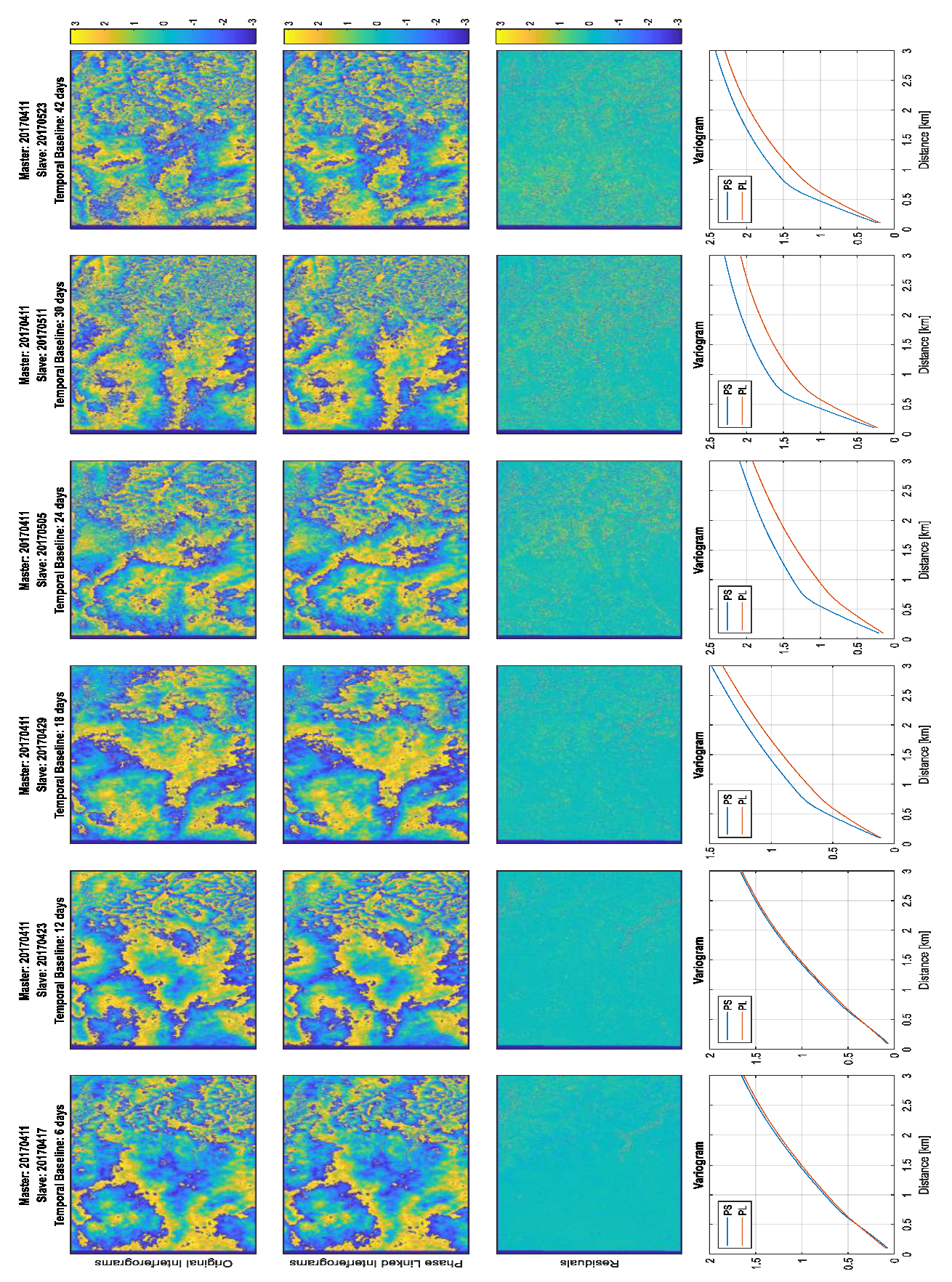
5.2. Processing
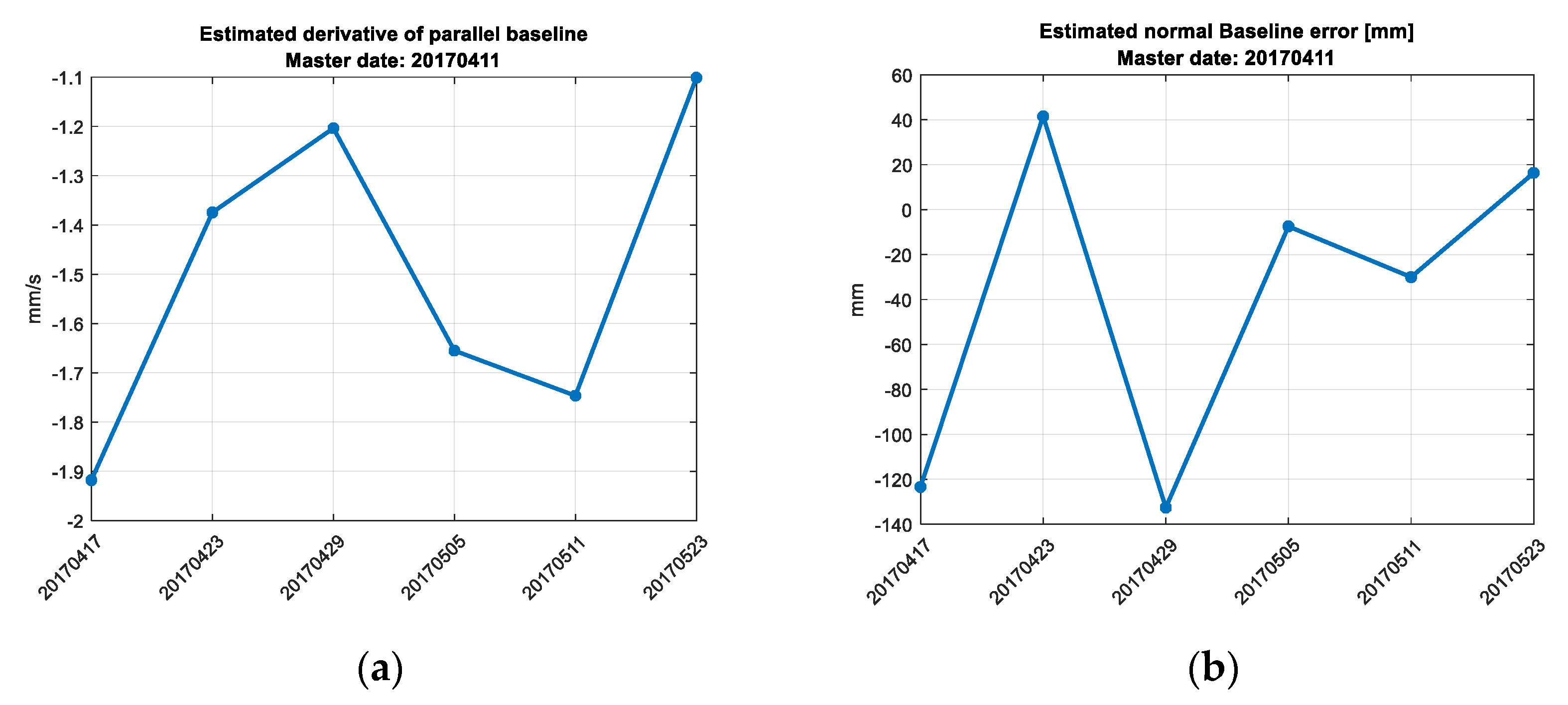
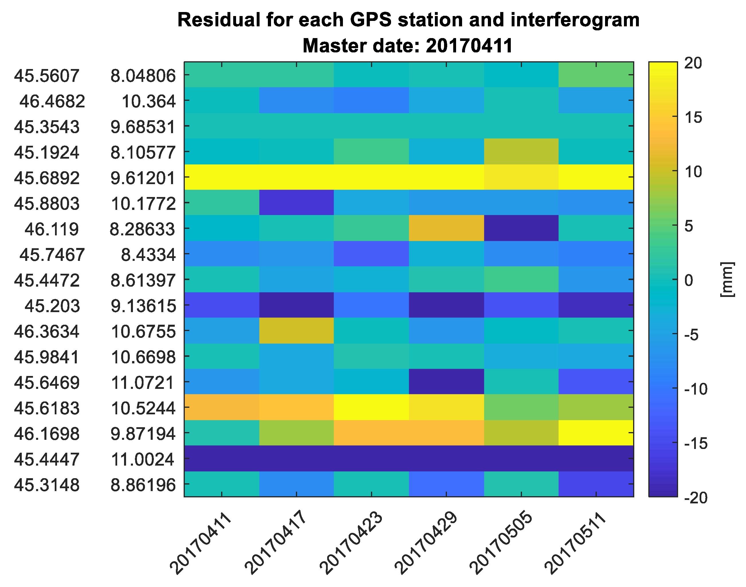
5.3. Orbit Correction
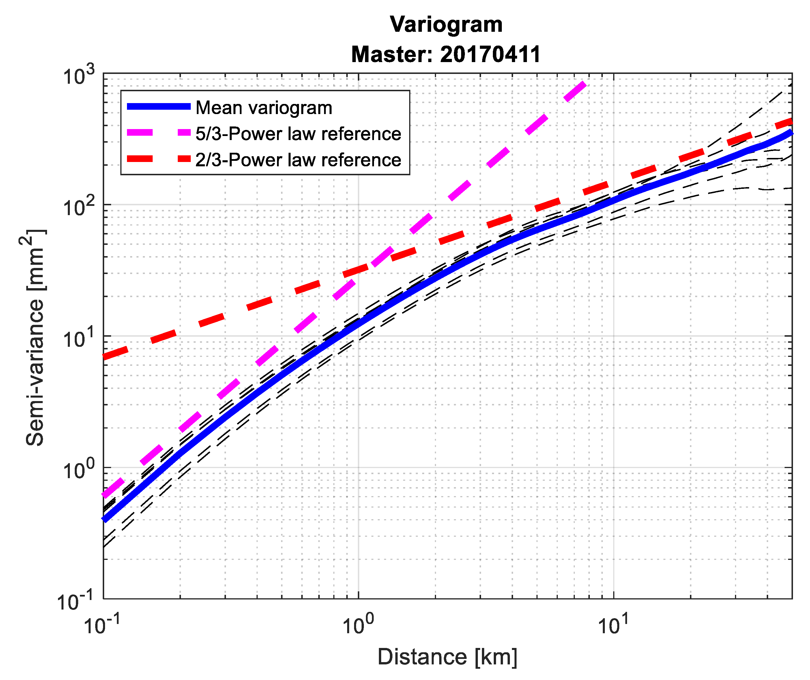
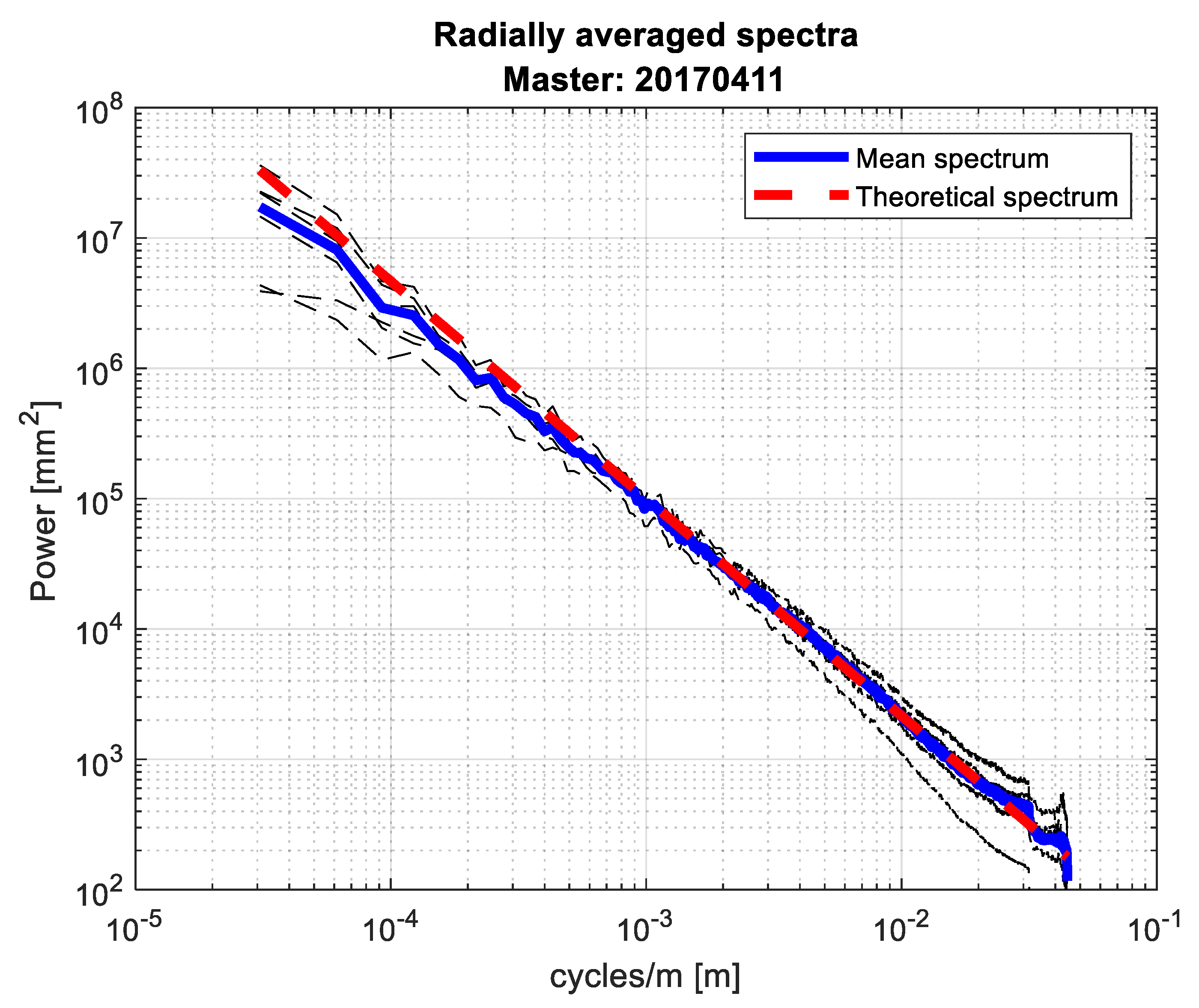
5.4. Variograms and Radially Average Spectra
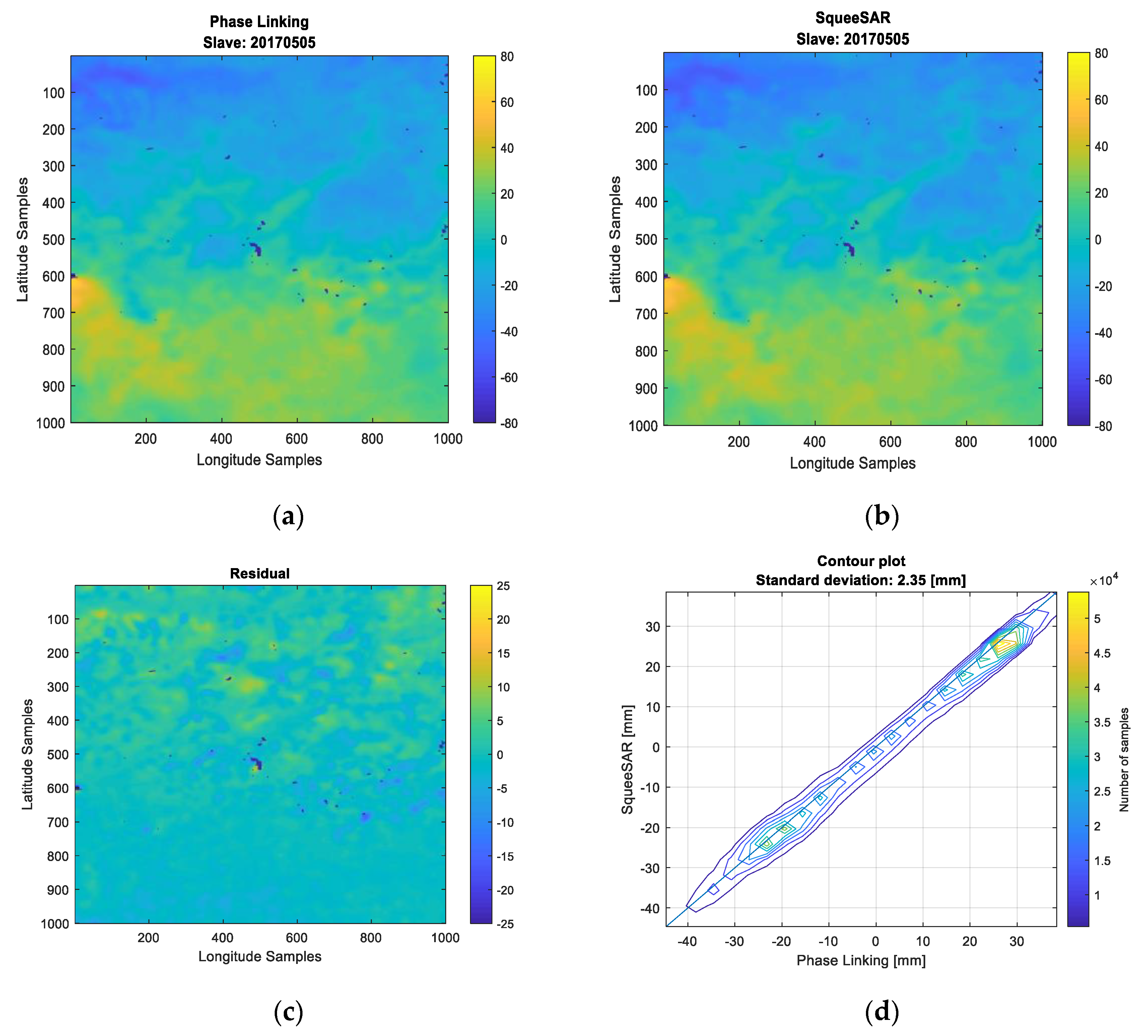
5.5. Comparison with Reference APS Maps from SqueeSAR®
5.6. A Note about GNSS and NWMP Comparison and NWMP Ingestion of SAR-Derived APS
6. Conclusions
Author Contributions
Funding
Acknowledgments
Conflicts of Interest
References
- Goldstein, R. Atmospheric limitations to repeat-track radar interferometry. Geophys. Res. Lett. 1995, 22, 2517–2520. [Google Scholar] [CrossRef] [Green Version]
- Tarayre, H.; Massonnet, D. Atmospheric Propagation heterogeneities revealed by ERS-1 interferometry. Atmos. Propag. Heterog. Reveal. ERS-1 Interferom. 1996, 23, 989–992. [Google Scholar] [CrossRef]
- Porcello, L.J. Turbulence-Induced Phase Errors in Synthetic-Aperture Radars. IEEE Trans. Aerosp. Electron. Syst. 1970, AES-6, 636–644. [Google Scholar] [CrossRef]
- Ferretti, A.; Prati, C.; Rocca, F. Permanent Scatterers in SAR Interferometry. IEEE Trans. Geosci. Remote Sens. 2001, 39, 13. [Google Scholar] [CrossRef]
- Ferretti, A.; Prati, C.; Rocca, F. Nonlinear subsidence rate estimation using permanent scatterers in differential SAR interferometry. IEEE Trans. Geosci. Remote Sens. 2000, 38, 2202–2212. [Google Scholar] [CrossRef] [Green Version]
- Biondi, F.; Clemente, C.; Orlando, D. An Atmospheric Phase Screen Estimation Strategy Based on Multichromatic Analysis for Differential Interferometric Synthetic Aperture Radar. IEEE Trans. Geosci. Remote Sens. 2019, 57, 7269–7280. [Google Scholar] [CrossRef]
- Monti Guarnieri, A.; Leanza, A.; Recchia, A.; Tebaldini, S.; Venuti, G. Atmospheric Phase Screen in GEO-SAR: Estimation and Compensation. IEEE Trans. Geosci. Remote Sens. 2018, 56, 1668–1679. [Google Scholar] [CrossRef]
- Ruiz Rodon, J.; Broquetas, A.; Monti Guarnieri, A.; Rocca, F. Geosynchronous SAR Focusing With Atmospheric Phase Screen Retrieval and Compensation. IEEE Trans. Geosci. Remote Sens. 2013, 51, 4397–4404. [Google Scholar] [CrossRef]
- Cong, X.; Balss, U.; Rodriguez Gonzalez, F.; Eineder, M. Mitigation of Tropospheric Delay in SAR and InSAR Using NWP Data: Its Validation and Application Examples. Remote Sens. 2018, 10, 1515. [Google Scholar] [CrossRef] [Green Version]
- Hu, Z.; Mallorquí, J.J. An Accurate Method to Correct Atmospheric Phase Delay for InSAR with the ERA5 Global Atmospheric Model. Remote Sens. 2019, 11, 1969. [Google Scholar] [CrossRef] [Green Version]
- Liu, S.; Hanssen, R.; Mika, A. On the value of high-resolution weather models for atmospheric mitigation in SAR interferometry. In Proceedings of the 2009 IEEE International Geoscience and Remote Sensing. Symposium, IEEE, Cape Town, South Africa, 12–17 July 2009; pp. II-749–II-752. [Google Scholar]
- Lagasio, M.; Parodi, A.; Pulvirenti, L.; Meroni, A.; Boni, G.; Pierdicca, N.; Marzano, F.; Luini, L.; Venuti, G.; Realini, E.; et al. A Synergistic Use of a High-Resolution Numerical Weather Prediction Model and High-Resolution Earth Observation Products to Improve Precipitation Forecast. Remote Sens. 2019, 11, 2387. [Google Scholar] [CrossRef] [Green Version]
- Mateus, P.; Miranda, P.M.A.; Nico, G.; Catalão, J.; Pinto, P.; Tomé, R. Assimilating InSAR Maps of Water Vapor to Improve Heavy Rainfall Forecasts: A Case Study With Two Successive Storms. J. Geophys. Res. Atmos. 2018, 123, 3341–3355. [Google Scholar] [CrossRef]
- Pichelli, E.; Ferretti, R.; Cimini, D.; Panegrossi, G.; Perissin, D.; Pierdicca, N.; Rocca, F.; Rommen, B. InSAR Water Vapor Data Assimilation into Mesoscale Model MM5: Technique and Pilot Study. IEEE J. Sel. Top. Appl. Earth Obs. Remote Sens. 2015, 8, 3859–3875. [Google Scholar] [CrossRef]
- Zebker, H.A.; Villasenor, J. Decorrelation in interferometric radar echoes. IEEE Trans. Geosci. Remote Sens. 1992, 30, 950–959. [Google Scholar] [CrossRef] [Green Version]
- Morishita, Y.; Hanssen, R.F. Temporal Decorrelation in L-, C-, and X-band Satellite Radar Interferometry for Pasture on Drained Peat Soils. IEEE Trans. Geosci. Remote Sens. 2015, 53, 1096–1104. [Google Scholar] [CrossRef]
- D’Aria, D.; Leanza, A.; Monti-Guarnieri, A.; Recchia, A. Decorrelating targets: Models and measures. In Proceedings of the 2016 IEEE International Geoscience and Remote Sens. Symposium (IGARSS), Beijing, China, 10–15 July 2016; pp. 3194–3197. [Google Scholar]
- Rocca, F. Modeling Interferogram Stacks. IEEE Trans. Geosci. Remote Sens. 2007, 45, 3289–3299. [Google Scholar] [CrossRef]
- Anghel, A.; Tudose, M.; Cacoveanu, R.; Datcu, M.; Nico, G.; Masci, O.; Dongyang, A.; Tian, W.; Hu, C.; Ding, Z.; et al. Compact Ground-Based Interferometric Synthetic Aperture Radar: Short-range structural monitoring. IEEE Signal Process. Mag. 2019, 36, 42–52. [Google Scholar] [CrossRef]
- Mateus, P.; Catalao, J.; Nico, G.; Benevides, P. Mapping Precipitable Water Vapor Time Series From Sentinel-1 Interferometric SAR. IEEE Trans. Geosci. Remote Sens. 2019, 58, 1–7. [Google Scholar] [CrossRef]
- Ferretti, A.; Fumagalli, A.; Novali, F.; Prati, C.; Rocca, F.; Rucci, A. A New Algorithm for Processing Interferometric Data-Stacks: SqueeSAR. IEEE Trans. Geosci. Remote Sens. 2011, 49, 3460–3470. [Google Scholar] [CrossRef]
- Lagasio, M.; Pulvirenti, L.; Parodi, A.; Boni, G.; Pierdicca, N.; Venuti, G.; Realini, E.; Tagliaferro, G.; Barindelli, S.; Rommen, B. Effect of the ingestion in the WRF model of different Sentinel-derived and GNSS-derived products: Analysis of the forecasts of a high impact weather event. Eur. J. Remote Sens. 2019, 52, 16–33. [Google Scholar] [CrossRef] [Green Version]
- Bamler, R.; Hartl, P. Synthetic aperture radar interferometry. Proc. IEEE 2000, 88, 333–382. [Google Scholar] [CrossRef]
- Moreira, A.; Prats-Iraola, P.; Younis, M.; Krieger, G.; Hajnsek, I.; Papathanassiou, K.P. A tutorial on synthetic aperture radar. IEEE Geosci. Remote Sens. Mag. 2013, 1, 6–43. [Google Scholar] [CrossRef] [Green Version]
- Belcher, D.P.; Rogers, N.C. Theory and simulation of ionospheric effects on synthetic aperture radar. IET Radar Sonar Navig. 2009, 3, 541. [Google Scholar] [CrossRef]
- Gomba, G.; Rodriguez Gonzalez, F.; De Zan, F. Ionospheric Phase Screen Compensation for the Sentinel-1 TOPS and ALOS-2 ScanSAR Modes. IEEE Trans. Geosci. Remote Sens. 2017, 55, 223–235. [Google Scholar] [CrossRef]
- Gomba, G.; Parizzi, A.; De Zan, F.; Eineder, M.; Bamler, R. Toward Operational Compensation of Ionospheric Effects in SAR Interferograms: The Split-Spectrum Method. IEEE Trans. Geosci. Remote Sens. 2016, 54, 1446–1461. [Google Scholar] [CrossRef] [Green Version]
- Hanssen, R. Radar Interferometry Data Interpretation and Error Analysis; Springer Science & Business Media: Berlin, Germany, 2001; Volume 2. [Google Scholar]
- Bähr, H.; Hanssen, R.F. Reliable estimation of orbit errors in spaceborne SAR interferometry: The network approach. J. Geod. 2012, 86, 1147–1164. [Google Scholar] [CrossRef] [Green Version]
- Tebaldini, S.; Monti, A. Methods and Performances for Multi-Pass SAR Interferometry. In Geoscience and Remote Sensing New Achievements; Imperatore, P., Riccio, D., Eds.; InTech: London, UK, 2010; ISBN 978-953-7619-97-8. [Google Scholar]
- Guarnieri, A.M.; Tebaldini, S. On the Exploitation of Target Statistics for SAR Interferometry Applications. IEEE Trans. Geosci. Remote Sens. 2008, 46, 3436–3443. [Google Scholar] [CrossRef]
- Ansari, H.; De Zan, F.; Bamler, R. Efficient Phase Estimation for Interferogram Stacks. IEEE Trans. Geosci. Remote Sens. 2018, 56, 4109–4125. [Google Scholar] [CrossRef]
- Ansari, H.; De Zan, F.; Gomba, G.; Bamler, R. EMI: Efficient Temporal Phase Estimation and its Impact on High-Precision InSAR Time Series Analysis. In Proceedings of the IGARSS 2019—2019 IEEE International Geoscience and Remote Sensing Symposium, Yokohama, Japan, 28 July–2 August 2019; pp. 270–273. [Google Scholar]
- Cao, N.; Lee, H.; Jung, H.C. A Phase-Decomposition-Based PSInSAR Processing Method. IEEE Trans. Geosci. Remote Sens. 2016, 54, 1074–1090. [Google Scholar] [CrossRef]
- Available online: https://gssc.esa.int/navipedia/index.php/Precise_Orbit_Determination (accessed on 12 February 2020).
- Bevis, M.; Businger, S.; Chiswell, S.; Herring, T.A.; Anthes, R.A.; Rocken, C.; Ware, R.H. GPS Meteorology: Mapping Zenith Wet Delays onto Precipitable Water. J. Appl. Meteorol. 1994, 33, 379–386. [Google Scholar] [CrossRef]
- Bevis, M.; Businger, S.; Herring, T.A.; Rocken, C.; Anthes, R.A.; Ware, R.H. GPS meteorology: Remote Sens. of atmospheric water vapor using the global positioning system. J. Geophys. Res. Atmos. 1992, 97, 15787–15801. [Google Scholar] [CrossRef]
- Realini, E.; Reguzzoni, M. goGPS: Open source software for enhancing the accuracy of low-cost receivers by single-frequency relative kinematic positioning. Meas. Sci. Technol. 2013, 24, 115010. [Google Scholar] [CrossRef]
- Hanssen, R.; Feijt, A.; Klees, R. Comparison of precipitable water vapor observations by spaceborne radar interferometry and Meteosat 6.7. J. Atmos. Ocean. Technol. 2000, 18, 756–764. [Google Scholar] [CrossRef] [Green Version]
- Tatarski, V.I.; Silverman, R.A.; Chako, N. Wave Propagation in a Turbulent Medium. Phys. Today 1961, 14, 46. [Google Scholar] [CrossRef]
- Williams, S.; Bock, Y.; Fang, P. Integrated satellite interferometry: Tropospheric noise, GPS estimates and implications for interferometric synthetic aperture radar products. J. Geophys. Res. Solid Earth 1998, 103, 27051–27067. [Google Scholar] [CrossRef]
- Treuhaft, R.N.; Lanyi, G.E. The effect of the dynamic wet troposphere on radio interferometric measurements. Radio Sci. 1987, 22, 251–265. [Google Scholar] [CrossRef]


| Requirement for High Res NWPMs | Threshold | Breakthrough | Goal |
|---|---|---|---|
| Temporal Resolution | 6 h | 60 min | 15 min |
| Spatial Resolution | 20 km | 5 km | 0.5 km |
| Sensor | Mode | Scene Size | Error in Range and Azimuth | |||
|---|---|---|---|---|---|---|
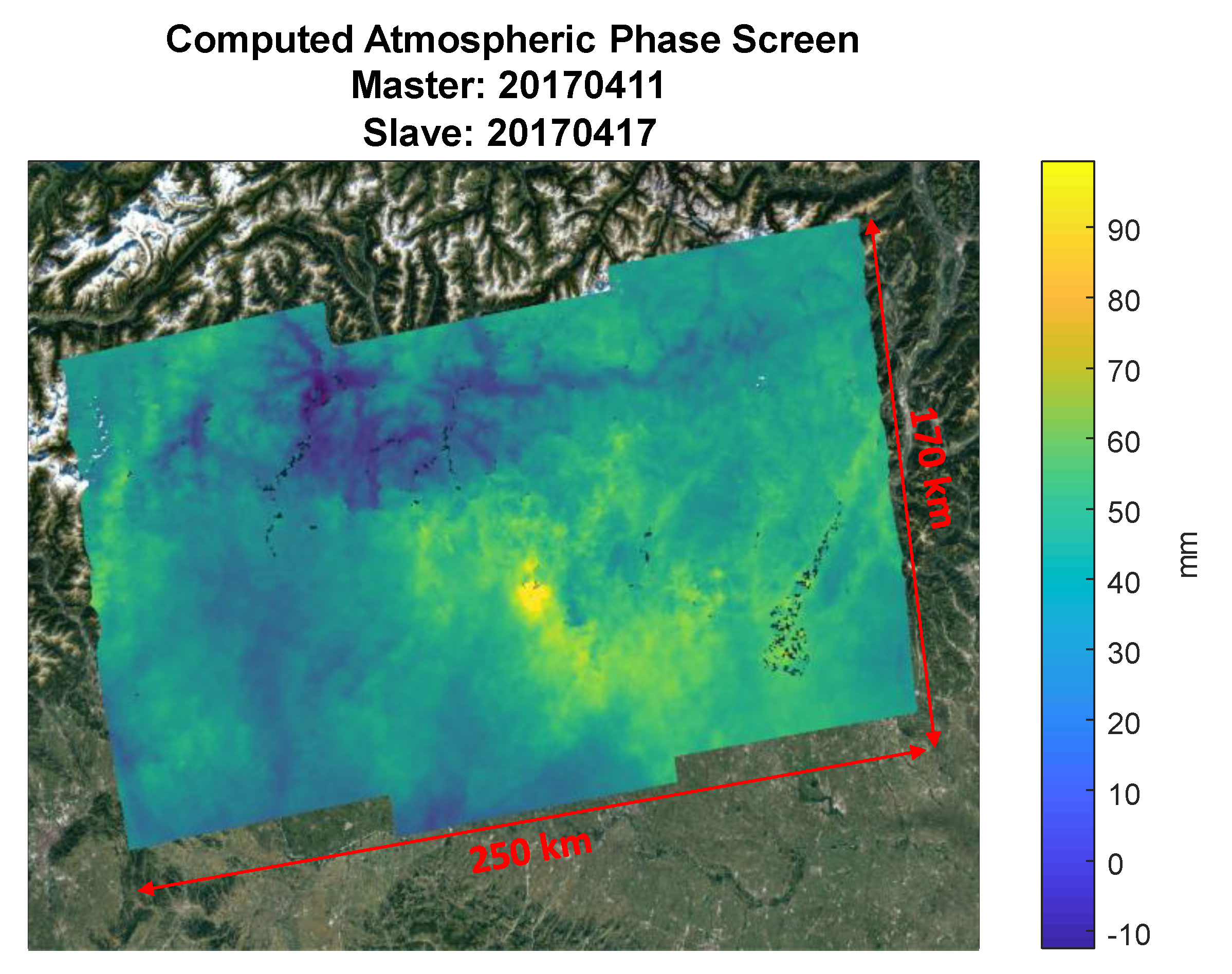
| Sentinel-1 | IW | 5.6 cm | 250 km × 170 km | 11 cm | 1.1 mm/s | 28 mm |
| Date | Temporal Baseline w.r.t. Master (Days) | Temporal Baseline w.r.t. Previous Image (Days) |
|---|---|---|
| 11 April 2017 | 0 | - |
| 17 April 2017 | 6 | 6 |
| 23 April 2017 | 12 | 6 |
| 29 April 2017 | 18 | 6 |
| 5 May 2017 | 24 | 6 |
| 11 May 2017 | 30 | 6 |
| 23 May 2017 | 42 | 12 |
| Date | Temporal Baseline w.r.t. Master (Days) | Temporal Baseline w.r.t. Previous Image (Days) | Standard Deviation (mm) |
|---|---|---|---|
| 11 April 2017 (master) | 0 | - | - |
| 17 April 2017 | 6 | 6 | 2.25 |
| 23 April 2017 | 12 | 6 | 2.32 |
| 29 April 2017 | 18 | 6 | 2.08 |
| 5 May 2017 | 24 | 6 | 2.35 |
| 11 May 2017 | 30 | 6 | 2.75 |
| 23 May 2017 | 42 | 12 | 2.81 |
© 2020 by the authors. Licensee MDPI, Basel, Switzerland. This article is an open access article distributed under the terms and conditions of the Creative Commons Attribution (CC BY) license (http://creativecommons.org/licenses/by/4.0/).
Share and Cite
Manzoni, M.; Monti-Guarnieri, A.V.; Realini, E.; Venuti, G. Joint Exploitation of SAR and GNSS for Atmospheric Phase Screens Retrieval Aimed at Numerical Weather Prediction Model Ingestion. Remote Sens. 2020, 12, 654. https://doi.org/10.3390/rs12040654
Manzoni M, Monti-Guarnieri AV, Realini E, Venuti G. Joint Exploitation of SAR and GNSS for Atmospheric Phase Screens Retrieval Aimed at Numerical Weather Prediction Model Ingestion. Remote Sensing. 2020; 12(4):654. https://doi.org/10.3390/rs12040654
Chicago/Turabian StyleManzoni, Marco, Andrea Virgilio Monti-Guarnieri, Eugenio Realini, and Giovanna Venuti. 2020. "Joint Exploitation of SAR and GNSS for Atmospheric Phase Screens Retrieval Aimed at Numerical Weather Prediction Model Ingestion" Remote Sensing 12, no. 4: 654. https://doi.org/10.3390/rs12040654