Article

Feasibility of Using MODIS Products to Simulate Sun-Induced Chlorophyll Fluorescence (SIF) in Boreal Forests

1
Key Laboratory of Geographical Processes and Ecological Security in Changbai Mountains, Ministry of Education, School of Geographical Sciences, Northeast Normal University, Changchun 130024, China
2
Northeast Institute of Geography and Agricultural Ecology, Chinese Academy of Science, Changchun 130102, China
*
Author to whom correspondence should be addressed.
The two authors have the same contribution.
Remote Sens. 2020, 12(4), 680; https://doi.org/10.3390/rs12040680
Submission received: 4 December 2019 / Revised: 18 February 2020 / Accepted: 18 February 2020 / Published: 19 February 2020

Abstract

:
Solar-induced chlorophyll fluorescence (SIF) is a novel approach to gain information about plant activity from remote sensing observations. However, there are currently no continuous SIF data produced at high spatial resolutions. Many previous studies have discussed the relationship between SIF and gross primary production (GPP) and showed a significant correlation between them, but few researchers have focused on forests, which are one the most important terrestrial ecosystems. This study takes Greater Khingan Mountains, a typical boreal forest in China, as an example to explore the feasibility of using MODerate resolution Imaging Spectroradiometer (MODIS) products and Orbiting Carbon Observatory-2 (OCO-2) SIF data to simulate continuous SIF at higher spatial resolutions. The results show that there is no significant correlation between SIF and MODIS GPP at a spatial resolution of 1 km; however, significant correlations between SIF and the enhanced vegetation index (EVI) were found during growing seasons. Furthermore, the broadleaf forest has a higher SIF than coniferous forest because of the difference in leaf and canopy bio-chemical and structural characteristic. When using MODIS EVI to model SIF, linear regression models show average performance (R2 = 0.58, Root Mean Squared Error (RMSE) = 0.14 from Julian day 145 to 257) at a 16-day time scale. However, when using MODIS EVI and temperature, multiple regressions perform better (R2 = 0.71, RMSE = 0.13 from Julian day 145 to 241). An important contribution of this paper is the analysis of the relationships between SIF and vegetation indices at different spatial resolutions and the finding that the relationships became closer with a decrease in spatial resolution. From this research, we conclude that the SIF of the boreal forest investigated can mainly be explained by EVI and air temperature.

Graphical Abstract

1. Introduction

Forests are important terrestrial ecosystems which contribute more than 70% of the terrestrial carbon pool [1]. Monitoring the status of forests from space is important for forest management [2]. Remote sensing has provided many global vegetation indices which rely on canopy reflectance in different spectral channels and has been widely used in forest research [3,4,5,6]. Over the past 30+ years, vegetation remote sensing based on “greenness” vegetation indices has greatly improved our understanding of the biosphere at a large scale. However, the vegetation indices (VIs) only explore the “potential photosynthesis” through “greenness”. Conversely, chlorophyll fluorescence has a unique ability to provide information about actual photosynthesis. For this reason, remote sensing of vegetation chlorophyll fluorescence has been a key research topic in the last 15 years [7,8,9].
Solar-induced chlorophyll fluorescence (SIF) is emitted by chlorophyll molecules and has been shown to be a proxy of photosynthetic activity [8,10,11,12]. As SIF is in competition with photochemical conversion, it may have the potential to estimate carbon cycles. During photosynthesis, the light absorbed by chlorophyll is used in the carbon fixation process, dissipated into heat, and re-emitted by chlorophyll a in the red and near infrared (NIR) spectral region [11,13,14]. The third part is called SIF, which is less than 5% of the total light absorbed by a plant; however, it offers a more direct measure of photosynthetic activity [15]. SIF provides a direct approach to diagnosing the actual functional status of vegetation, and the fluorescence signal can be quantified by passive (i.e., without artificial excitation sources) remote sensing systems exploiting the dark line of the solar and atmospheric spectra where irradiance is strongly reduced (Fraunhofer lines). In particular, two telluric O2 absorption bands (O2-B band at 687 nm and O2-A band at 760.4 nm) have been extensively used to estimate SIF because of their spectral proximity to the peaks of the fluorescence emission spectrum positioned at about 685 and 740 nm [2,16]. The recent advancement of satellite-based measurements of SIF provides tremendous potential for the global monitoring of terrestrial photosynthesis and the carbon cycle [11].
Global annual averaged SIF at 755 nm at a spatial resolution of 2° × 2° was derived from Greenhouse gases Observing SATellite (GOSAT) data for the first time by Frankenberg, et al. [15]. SIF data have been derived from Global Ozone Monitoring Experiment 2 (GOME-2), Scanning Imaging Absorption spectrometer for Atmospheric CHartograhY (SCIAMACHY), the Orbiting Carbon Observatory-2 (OCO-2), and TROPOspheric Monitoring Instrument (TROPOMI) satellites to promote the development of SIF remote sensing [7,10,13,17,18,19,20]. The FLuorescence EXplorer (FLEX) is the 8th ESA Earth Explorer mission that is planned for launch by 2024; this will provide the first 300 m resolution SIF imagery [21,22,23,24,25,26]. Most of the atmospheric chemistry satellites (GOSAT, GOME-2, SCHIAMACHY, OCO-2, and TROPOMI) mainly offer far-red SIF observations, while red SIF is available only from GOME-2 and SCHIAMACHY [14,20,27,28,29].
Different types of vegetation are usually characterized by different SIF values. In general, the highest SIF emissions are found in croplands, followed by broadleaf and then coniferous forests [30]. Due to the advantages of SIF in measuring vegetation photosynthesis, many researchers explored the potential of using SIF in modeling gross primary production (GPP). Some studies used MODIS products to simulate SIF at moderate spatial resolutions and obtained satisfactory results [11,28,31,32,33]. During the daytime, SIF has a positive correlation with photochemistry in leaves and thus could be used as a valid proxy for GPP. This implies the possibility of using vegetation indices to simulate SIF. Li, et al. [11] used SIF data derived from OCO-2 and flux tower GPP data to study the relationship between them and found a strong correlation. Parazoo, et al. [34] concluded that SIF can be used to quantify GPP changes in response to meteorological drivers. Taking the Amazon rainforest as the study region, Köhler, et al. [13] revealed the response of SIF to instantaneous photosynthetically active radiation (PAR). Although a surprisingly linear relationship was found at a regional or a global scale, the mechanistic link between SIF and GPP remains unclear [12,35] because the former closed relationships were statistically significant.
SIF provides a new perspective to estimate instantaneous vegetation and carbon-related processes that are essential for the assessment of carbon budgets of forest ecosystems [18]. This requires continuous SIF data at high spatial and temporal resolutions. However, continuous global coverage of SIF at a high spatial resolution cannot be generated due to the sparse spatial sampling mode of OCO-2 [10]. In this research, we explore the possibility of using MODIS and meteorological data to simulate SIF in a boreal forest of China. Our research provides robust evidence of the relationship between SIF and vegetation indices while demonstrating great potential for SIF simulation in boreal forests based on the enhanced vegetation index (EVI) and temperature.

2. Materials and Methods
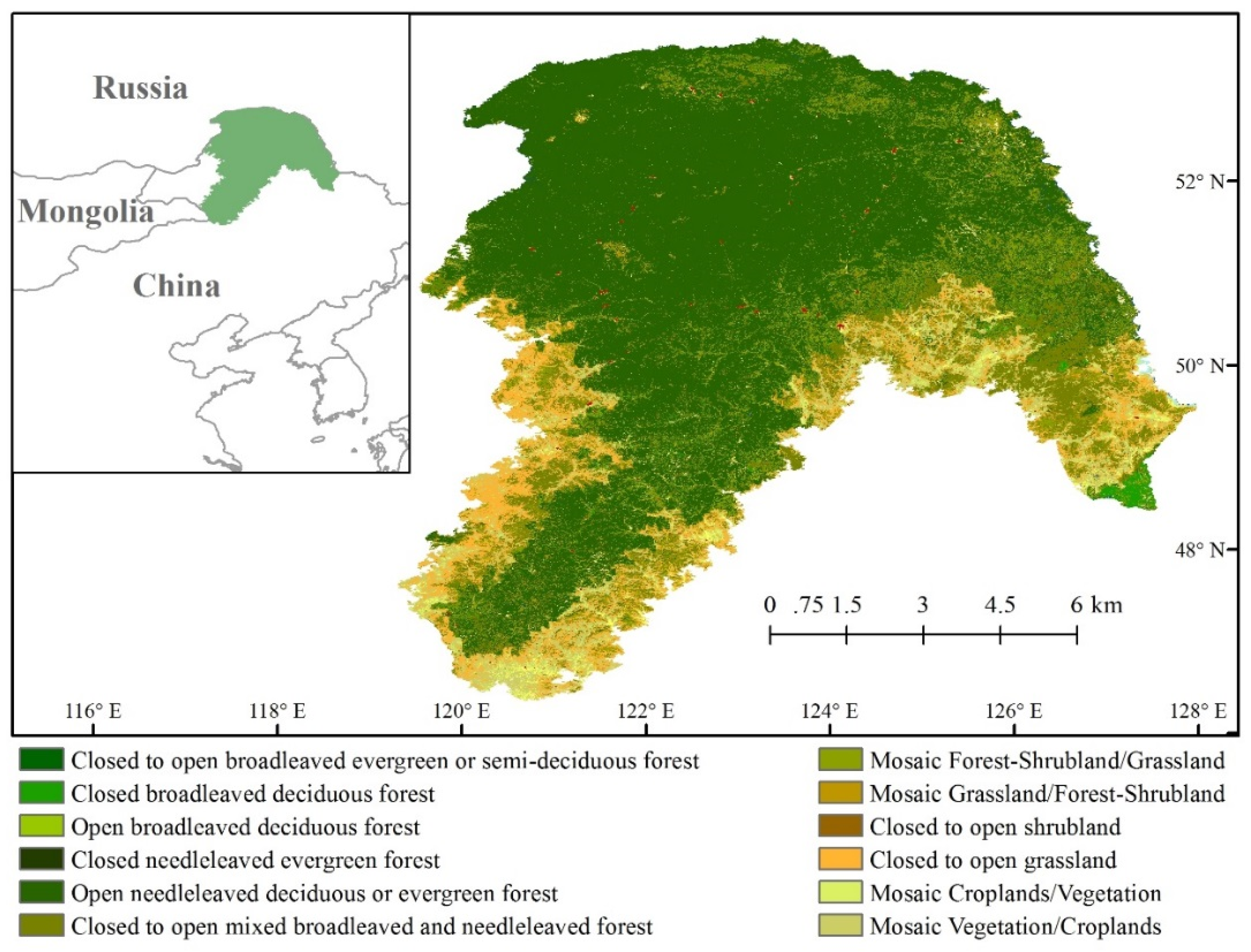
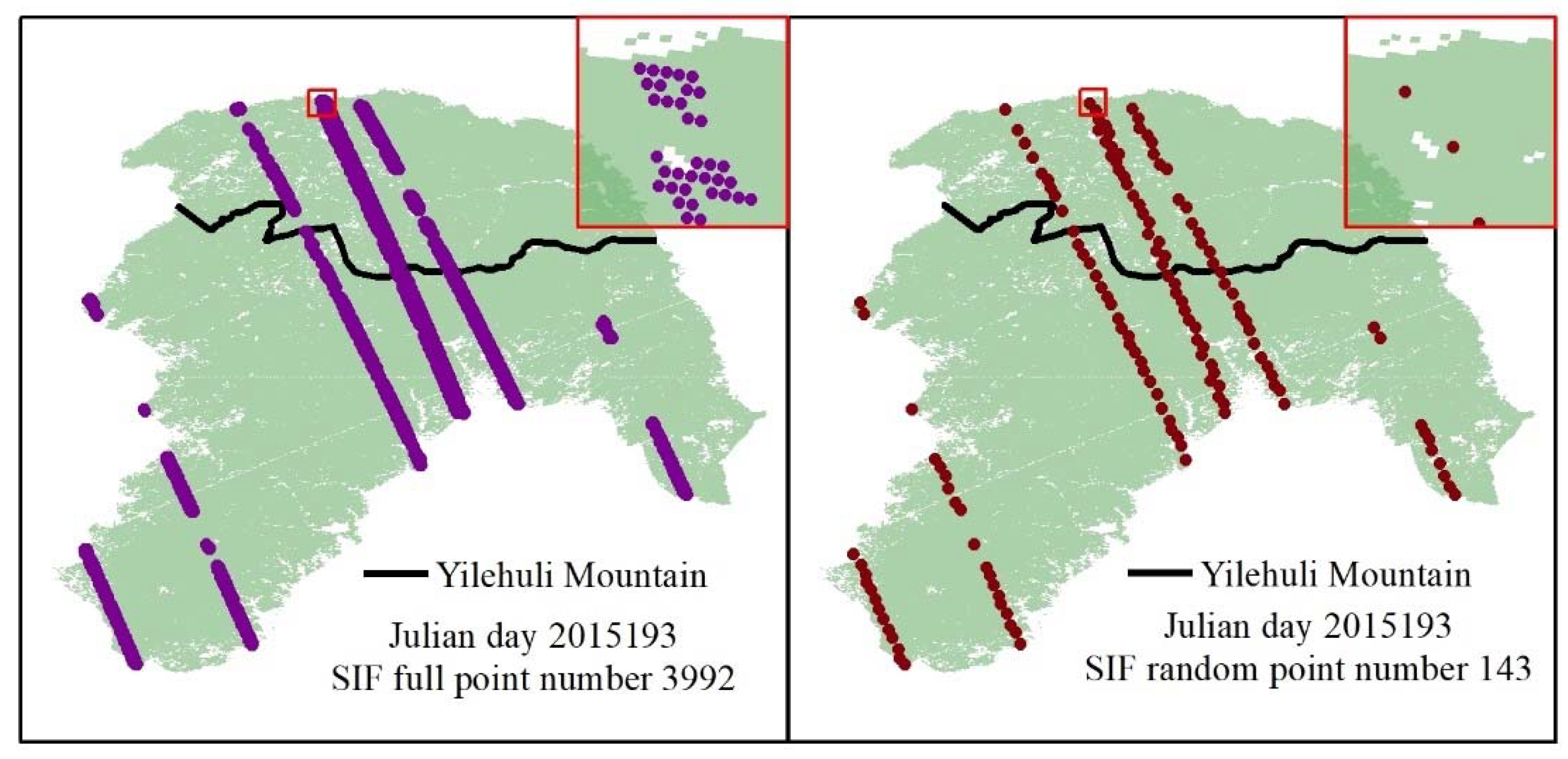
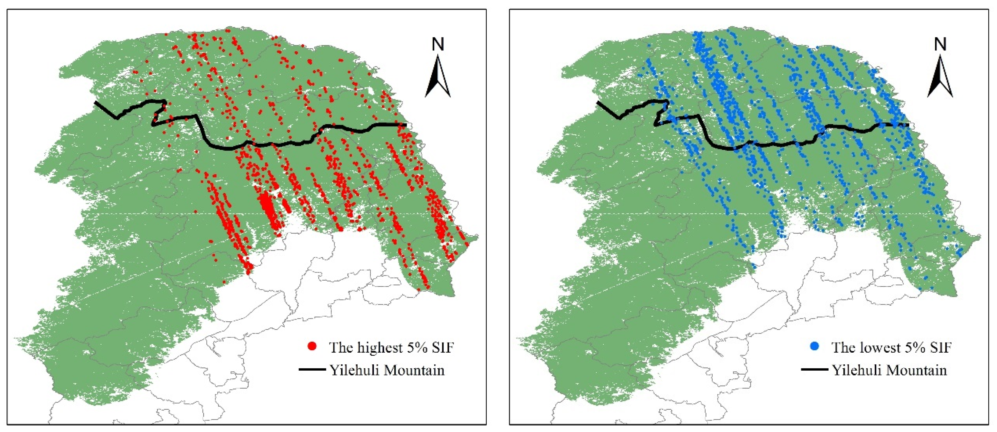
2.1. Study Region

Greater Khingan Mountains are part of the coniferous forests of northern Eurasia and the largest virgin forest in China with an area of 8.3 × 10⁶ hm2 (Figure 1). The direction of the main vein of Greater Khingan Mountains is NNE-SSW, and direction of the branch vein (the Yilehuli Mountain) is WWN-EES [36]. The region has a mountainous topography with elevation ranging from 260 m to 1700 m. The zonal vegetation in Greater Khingan Mountains is typical taiga dominated by Dahurian larch (Larix gmelinii), with areas of temperate and mixed broadleaf-conifer dominated by deciduous broadleaf birch (Betula platyphylla) and aspen (Populus davidiana and Populus suaveolens) [37].
The study region has cold temperate and continental monsoon climates with an annual average temperature of -2.8℃, mean annual maximum and minimum temperatures of 35℃ and -40℃, respectively, and mean annual precipitation of about 460 mm. The growing season in this area is relatively short (150 days), and the frost-free period is also relatively short (~80–100 days) [37]. The period between May 10 and September 14 (Julian period 145 to 257) was selected as the growing season to explore the possibility of using MODIS products to simulate SIF.
In this study, we aim to determine whether MODIS products can be used to estimate SIF in the boreal forest. The first step was to identify the forest. When compared MODIS NDVI with Landsat 8 Operational Land Imager (OLI) images, we found that when the normalized difference vegetation index (NDVI) in July is greater than 0.8, the land cover is forest. By using this threshold, the regional forest distribution of Greater Khingan Mountains was extracted to estimate SIF.

2.2. OCO-2 Data

The OCO-2 satellite, launched on July 2, 2014, is one of the National Aeronautics and Space Administration’s (NASA) mission satellite designed to monitor CO2 concentrations in the atmosphere. It ascends across the equator at 1:30 Local Standard Time (LST) and has a 16-day re-visit time. Each second, OCO-2 acquires 24 data points with a ground pixel size of 1.3 km × 2.25 km.
A novel data product of OCO-2 is SIF, which was evaluated at 757 nm and 770.1 nm of the OCO-2 O2 A-band, and is considered an indicator of the plant functional status [12,28]. OCO-2 acquires data in three different observation modes: nadir, glint, and target. Nadir mode is used to view the ground directly below the spacecraft. Glint mode is used when tracking near the location with direct, reflected sunlight. Target mode collects a large number of measurements from calibration/validation sites [40].
In this study, cloud-free nadir observations of offset-corrected OCO-2 SIF (Version 8r) were used to explore the relationship between MODIS products and SIF at a regional scale. We averaged both OCO-2 SIF retrieval results (valid at 757 and 770.1 nm) after multiplying SIF at 770.1 with 1.7 to account for the decrease in the wavelength of SIF in this part of the spectrum, as documented in the OCO-2 Data Product User’s Guide and Yu, et al. [41]. To make SIF data more reasonable, we deleted SIF values lower than 0.1 W m−2 µm−1 sr−1.

2.3. MODIS Products

MODIS is a key instrument aboard the satellites Terra (which crosses the equator in the morning) and Aqua (which crosses the equator in the afternoon). Terra MODIS and Aqua MODIS sample the entirety of Earth’s surface in a 2330-km swath, providing near-global daily coverage. MODIS acquires data in 36 spectral bands from 0.4 to 14.4 μm at three spatial resolutions: 250 m (bands 1 and 2), 500 m (band 3-7), and 1,000 m (band 8-36). It covers visible, near-infrared, shortwave infrared, and thermal-IR regions in the electro-magnetic spectrum [6,38,42].
Many MODIS products at different spatial and temporal scales have been released on an official website. They are freely downloadable and have been widely used in many studies. MODIS NDVI, EVI, leaf area index (LAI), fraction of absorbed photosynthetically active radiation (FAPAR), and GPP were used in this study. NDVI and EVI were extracted from MOD13A2, with 1 km spatial resolution and a 16-day composite. LAI and FAPAR, with a 500 m spatial resolution and 8-day composite, were extracted from MOD15A2H. GPP were extracted from MOD17A2H at a spatial resolution of 500 m and 8-day composite. All data were downloaded from https://ladsweb.modaps.eosdis.nasa.gov.

2.4. Meteorological Data

The meteorological data in this study contain two parts: one is MERRA-2, a reanalysis data product from NASA/GMAO (Global Modeling and Assimilation Office) with a resolution of 0.5° × 0.625°. Daily surface downwelling PAR data from MERRA-2 [43] were selected to analyze their relationship with SIF. The other meteorological data used in this study are temperature and precipitation data from the National Meteorological Information Center (NMIC, http://data.cma.cn/).

2.5. Data Processing

To maintain the concordance between MODIS and OCO-2 data, we selected a 16-day temporal resolution at a spatial resolution of 1 km. FAPAR, LAI, and GPP data were resampled to 1 km and compiled to 16 days using the maximum value composition (MVC) technique [44]. As mentioned above, the re-visit cycle of OCO-2 is 16 days, and point data were obtained during its clear-sky overpass. SIF data were also compiled in 16 days and grouped according to MODIS products. To avoid spatial autocorrelation, 200 SIF points were randomly selected every day for 16 days to calculate their relationship with vegetation. Squares with 1 km length that cover the study region were built, and then the mean value of SIF and the vegetation index values of NDVI, EVI, LAI, FAPAR, and GPP within each square were extracted.

3. Results

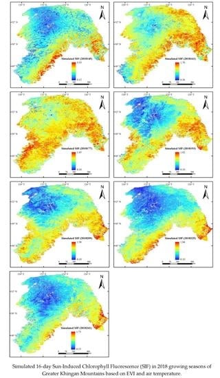
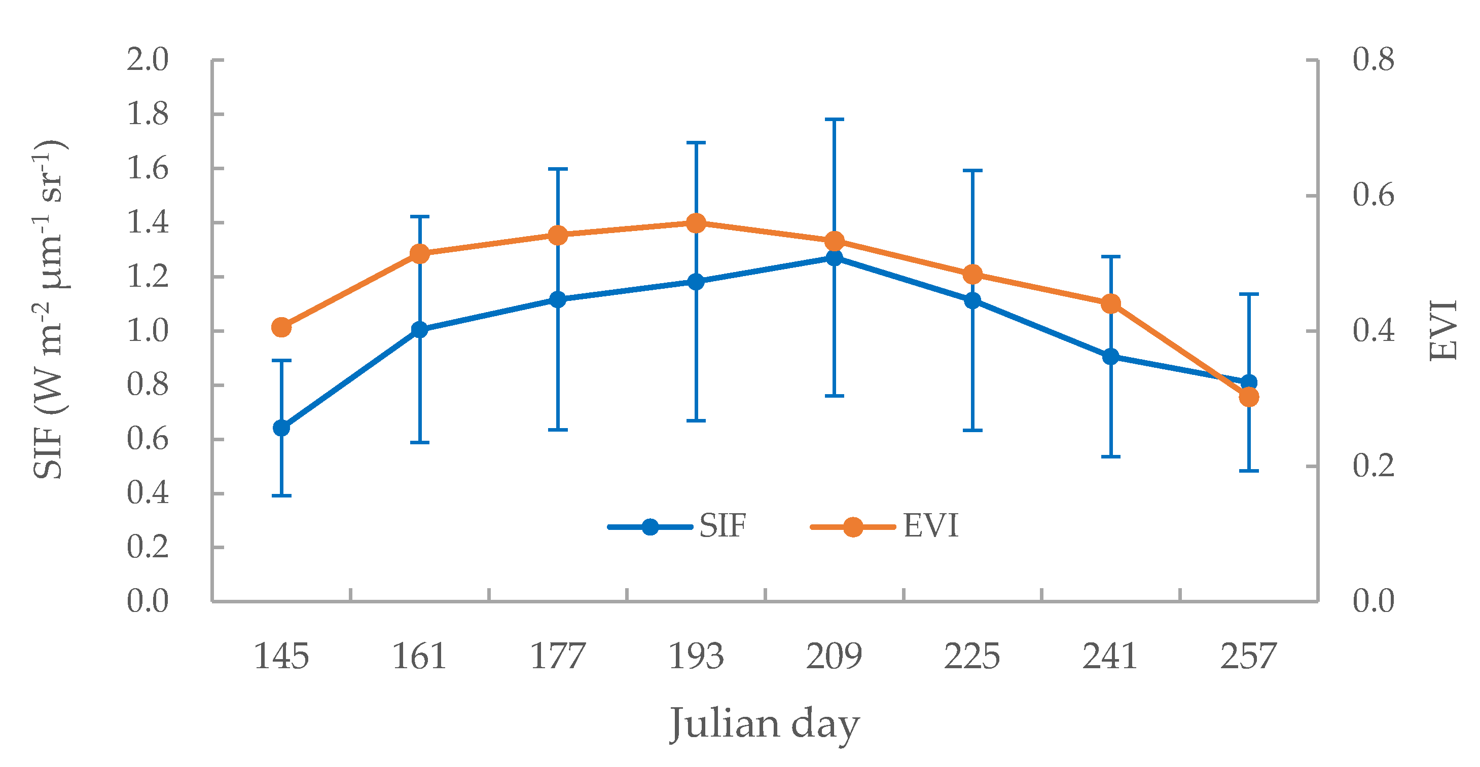
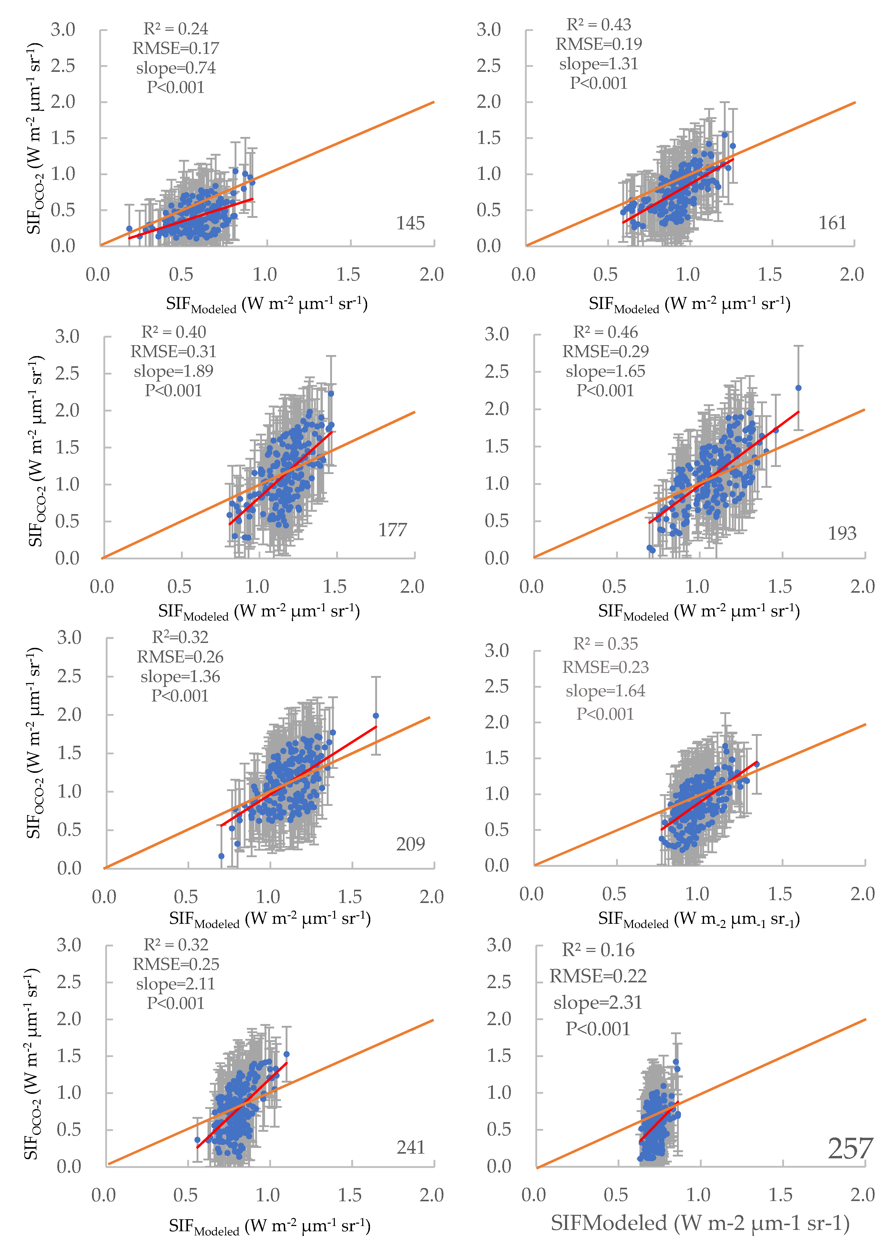
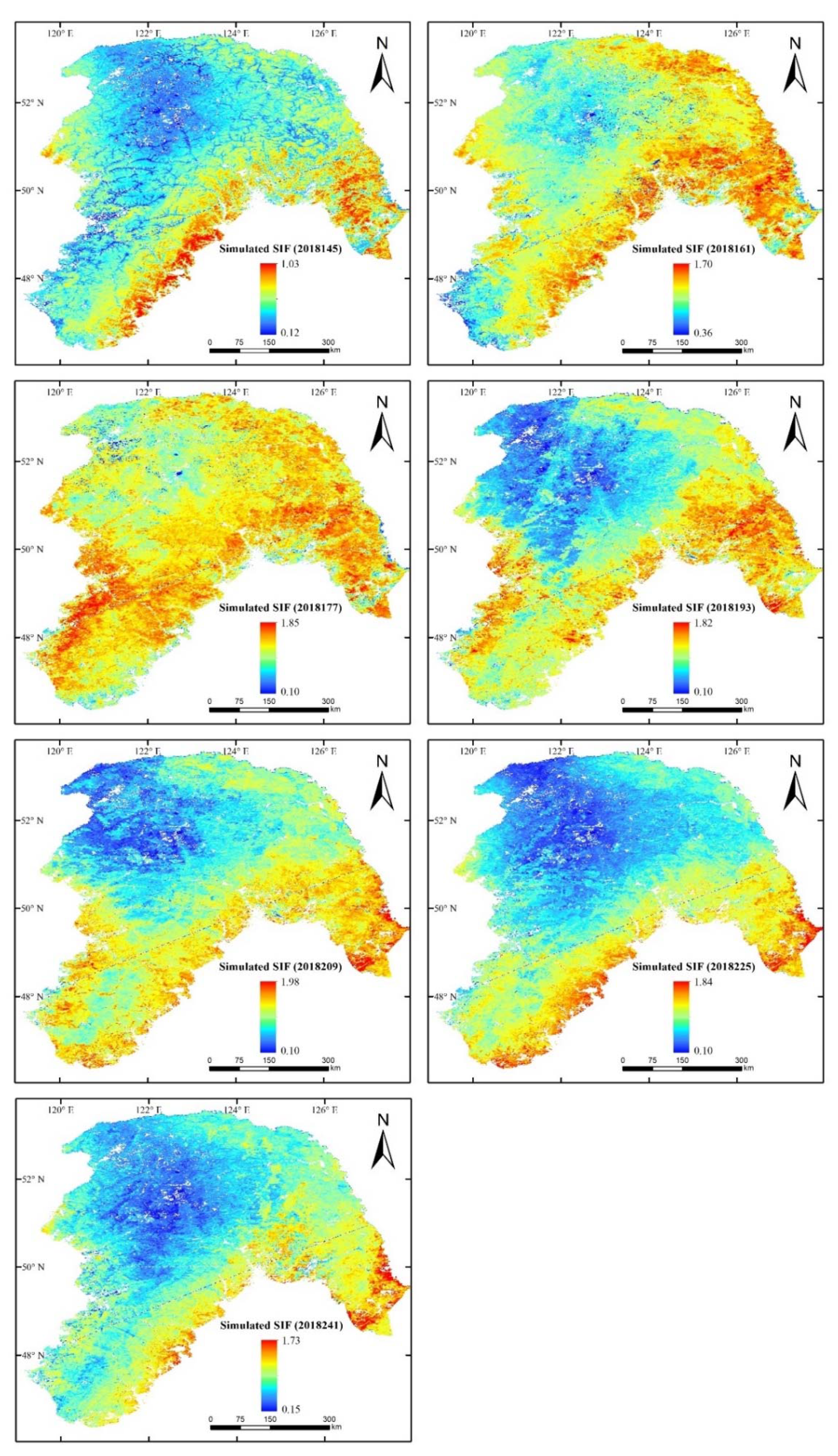
3.1. Temporal Variation of SIF in the Large Study Area

We calculated the average SIF and EVI values of the study region for each of the 16 days from 2015 to 2018 (Figure 2). During the beginning of the growing season, SIF increased from Julian day 145 (May 10-25) and reached its peak value on Julian day 209 (July 13–28), before subsequently decreasing. Autumn arrives early in the study region of Greater Khingan Mountains because of higher latitudes (at 46°–53° N), and on Julian day 257 (October 30–September 14) the SIF value was quite low. The SIF and EVI curves show similar change trend, but the peak value of SIF lags behind that of EVI. Figure 2 shows that the trend of the SIF values was quite similar to the plant growth cycle, and SIF has been advised in phenology studies.

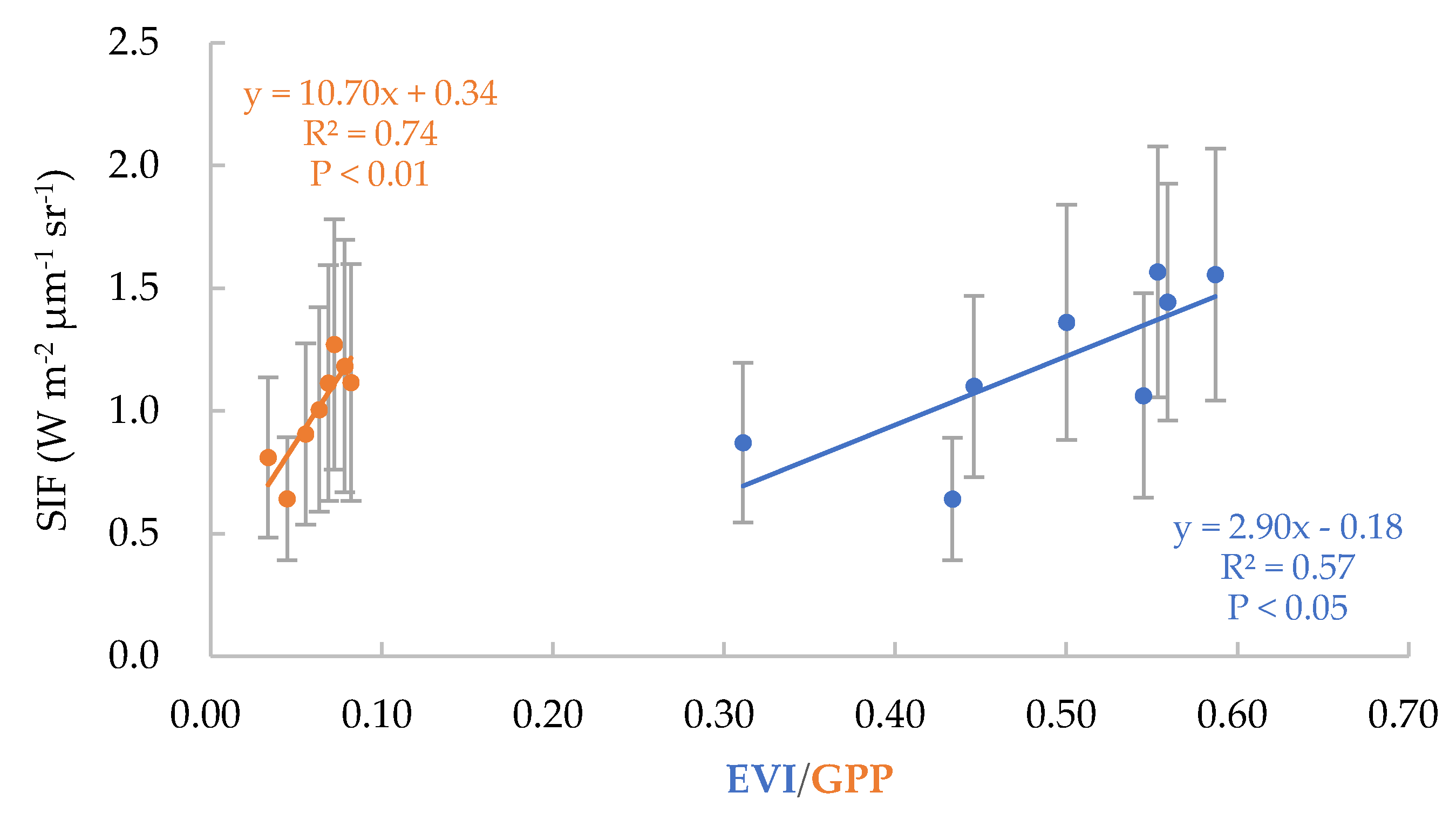
3.2. SIF–EVI and SIF–GPP at a Regional Scale

To understand the relationships of SIF–EVI and SIF–GPP at the regional scale, the mean values of EVI, GPP, and SIF for the study region were calculated for each 16-day period, and a scatter plot was drawn (Figure 3). Here, the MODIS GPP product was used to represent the true GPP value. The relationship between SIF and GPP (R2 = 0.74, n = 8, P < 0.01) was closer than that between SIF and EVI (R2 = 0.57, n = 8, P < 0.05). This shows that, at a regional scale, EVI and GPP had significant correlations with SIF. The slope between SIF and EVI was 2.90, and the value between SIF and GPP was 10.70. However, this result only reflects the relationships at a regional scale. To understand more accurate relationships between vegetation indices and SIF, a more detailed analysis at a local scale is needed.

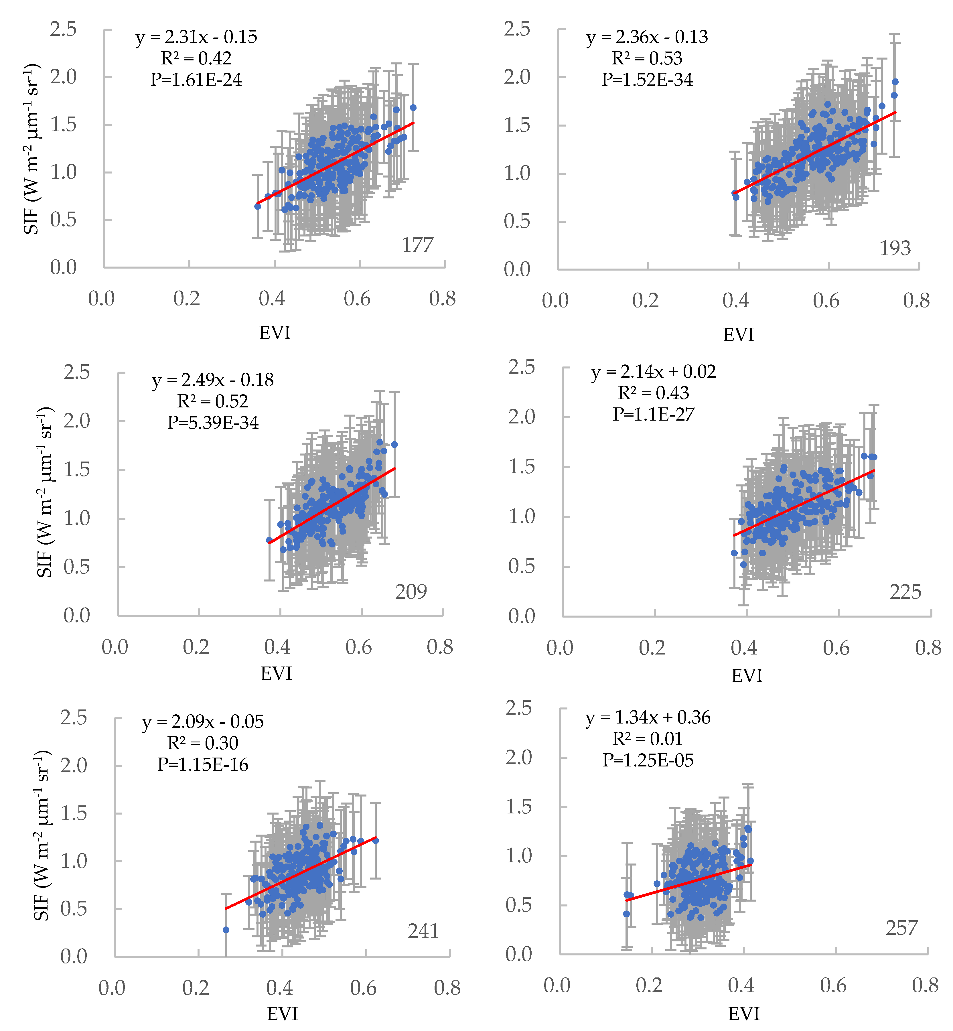
3.3. Relationships of SIF–EVI at a Local Scale

Greater Khingan Mountains contain cold-temperate coniferous forests dominated by Dahurian larch (Larix gmelinii). The branch vein of Yilehuli Mountain divides Greater Khingan Mountains into two slope directions, Lingnan (the southern slope of the mountains) and Lingbei (the northern slope of the mountains) (Figure 4). The broadleaf tree ratio in the south of Yilehuli Mountain is higher than that in the north [36], and a broadleaf tree usually has a higher LAI than a needle leaf tree.
To understand the relationship between vegetation indices and SIF, vegetation index values corresponding to OCO-2 SIF points were extracted. Thanks to the highly efficient data acquisition techniques of OCO-2, there are thousands of SIF data points and density distributions over the course of 16 days. To eliminate the spatial autocorrelation in SIF, we randomly selected 200 points with point distances longer than 5 km (on some Julian days, the random points did not reach 200). Figure 4 shows an example of random point extraction on Julian day 2015193.
SIF can reflect a part of actual photosynthesis. NDVI and EVI are the vegetation indices that reflect vegetation greenness, and EVI is widely used in forest regions because it is less affected by the saturation effect compared to the NDVI [33]. Significant correlations (P < 0.05) between SIF and EVI in the growing seasons in 2015 and 2016 were found (Figure 5), which are different from the results of former studies and those at a regional scale. The correlation coefficients of SIF–NDVI, SIF–GPP, SIF–LAI, and SIF–FAPAR were also calculated, but no significant correlations were found.
The correlation coefficient between EVI and SIF changed over the course of 16 days; however, it steadily reached a peak value on Julian day 209 and subsequently decreased. This is similar to the pattern observed in Figure 2.

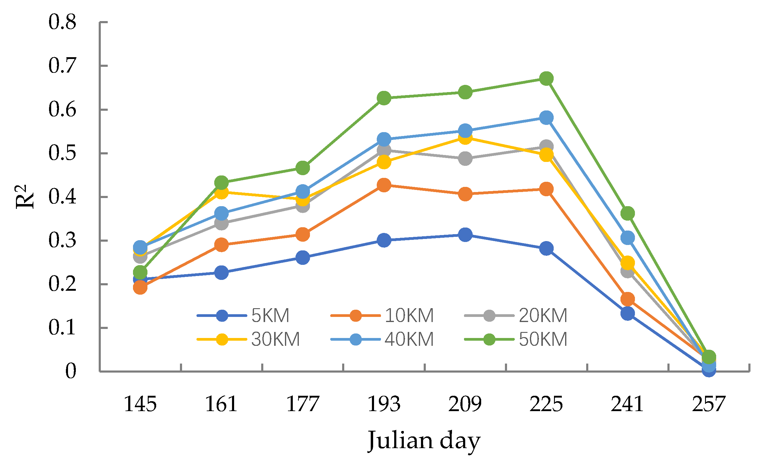
3.4. SIF–EVI Relationships at Different Spatial Resolutions

We examined the correlation between SIF and EVI at spatial resolutions of 5 km, 10 km, 20 km, 30 km, 40 km, and 50 km using the growing-season data from 2015 and 2016. The EVI was resampled to the corresponding spatial resolution, and average SIF values were obtained within each EVI pixel. From the result (Figure 6), we found that the R2 values were different for different spatial resolutions, with a clear trend of lower spatial resolution with higher R2 value. Between Julian days 177 and 241, R2 values for the 20 km and 30 km spatial resolutions were higher than that for 10 km but lower than that of the 40 km spatial resolution. On Julian days 193 and 225, R2 values of 20 km were higher than those of 30 km and on other days, R2 values of 30 km were higher than those of 20 km.

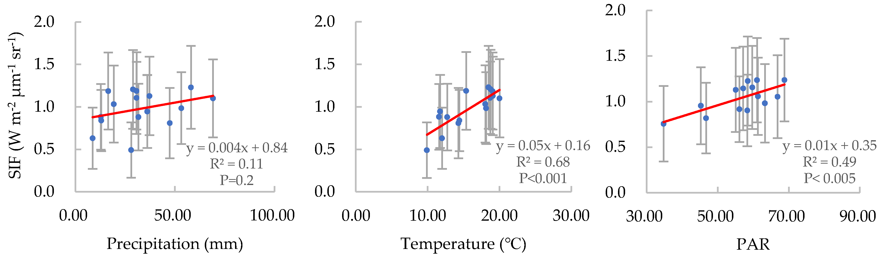
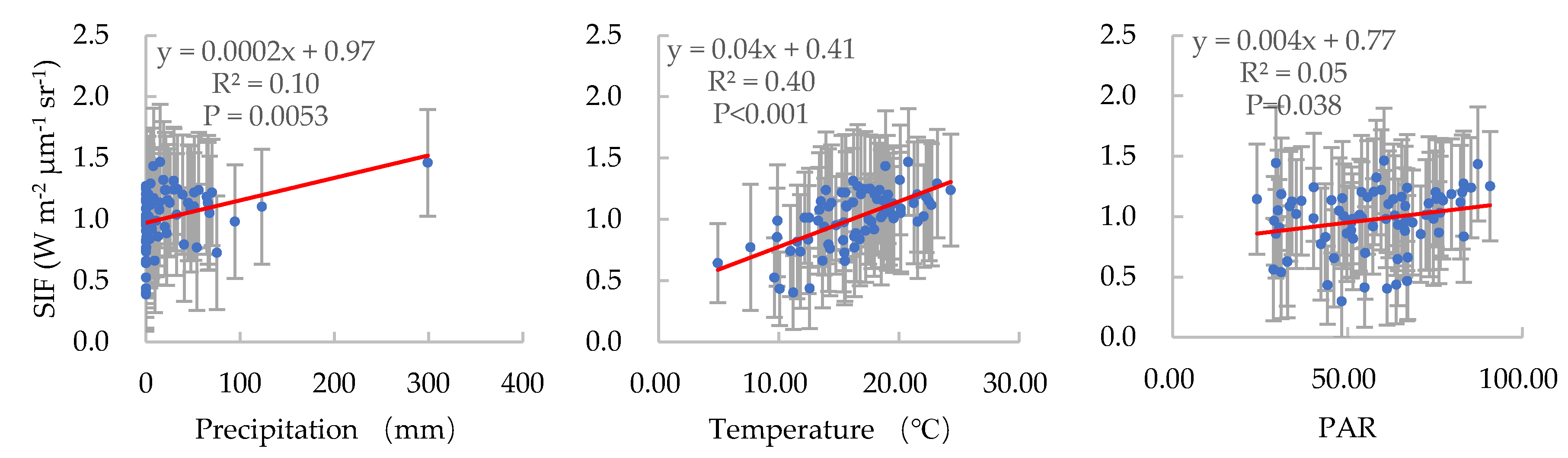
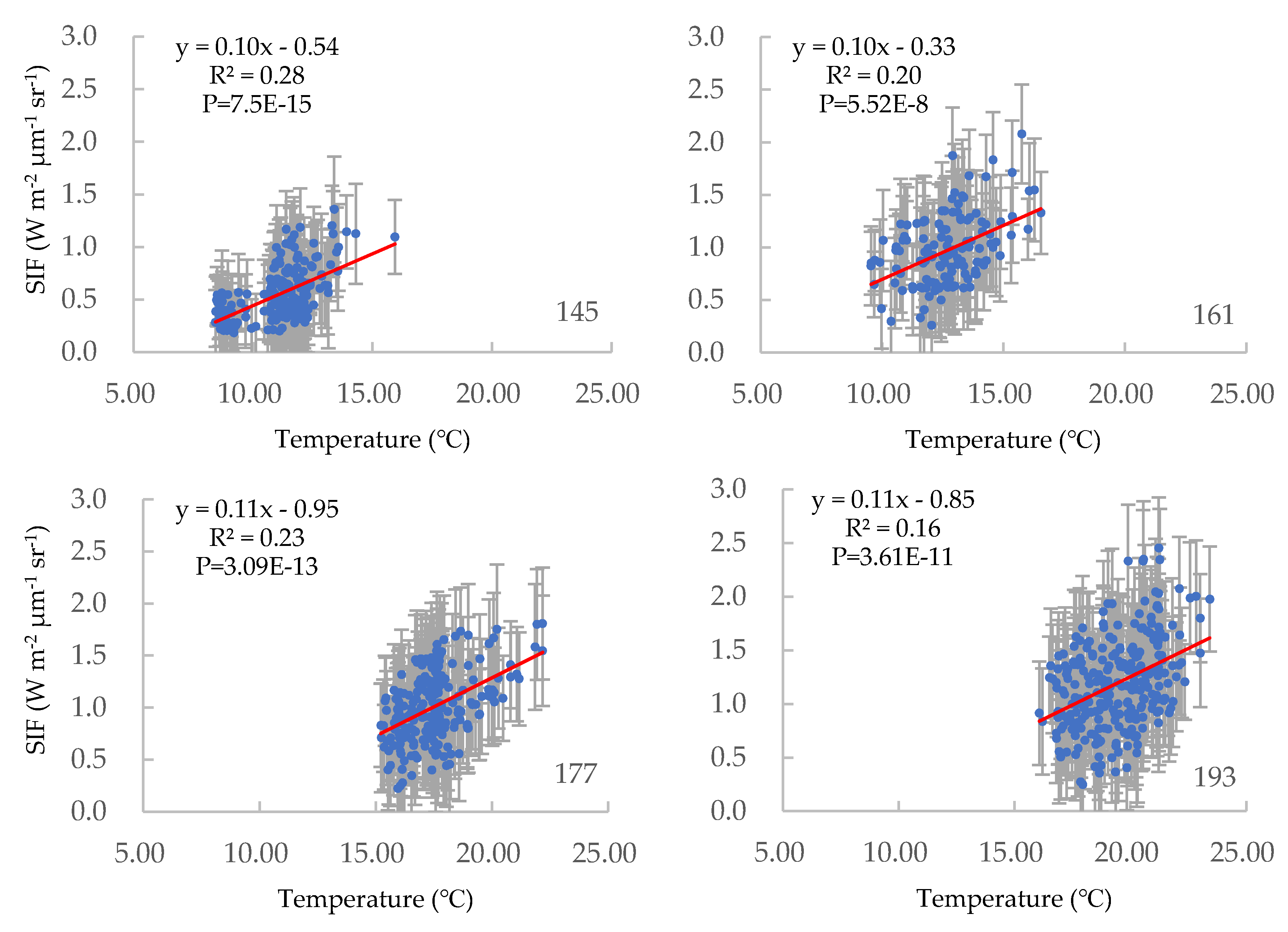
3.5. The Relationships between Meteorological Factors and SIF

Some researchers agree that SIF is affected by meteorological factors such as precipitation, temperature, and PAR [28,45,46,47]. We examined the relationships between SIF and meteorological factors on daily and 16-day time scale.
Figure 7 shows the relationships between SIF and meteorological factors at 16 days and at a regional scale. Significant correlations between SIF and temperature and SIF and radiation (R2 = 0.68, P < 0.001; R2 = 0.49, P = 0.005, respectively) were found. Precipitation had no significant correlation with SIF at the regional scale which indicated that precipitation was not the factor restraining plant growth in Greater Khingan Mountains.
Daily mean meteorological parameters and SIF at the regional scale were also calculated, and scatter plots were drawn (Figure 8). Only temperature had a significant correlation with SIF (R2 = 0.40, P < 0.001). Based on the significant correlations between SIF and temperature at both 16-day and daily time scales, we concluded that, at the regional scale, temperature may affect SIF via photosynthesis.
To understand the relationship between temperature and SIF at a 16-day time scale, we downloaded the daily mean temperatures of 27 ground stations within and around the study region in 2015 and 2016. We used kriging interpolation to obtain spatial continuous maps of air temperature (Figure 9). The results are shown in Figure 10. There was a significant correlation between SIF and temperature in the growing season, except on Julian day 257 when vegetation became yellow, and when the chlorophyll content decreased in the autumn. In the growing season, canopy capacity and SIF increased with increasing air temperatures.

4. Discussion

4.1. SIF Differences between Vegetation Types

To understand the SIF values between needle and broadleaf plants, we selected the highest 5% (among all 1519 SIF points) and lowest 5% (among all 1482 points) SIF values of each Julian day and analyzed the spatial distribution of high and low SIF values. We found that 77.75% (1181 out of 1519) of the highest SIF values and 69.23% (1026 out of 1482) of the lowest SIF values were distributed in the southern and northern Yilehuli Mountain, respectively (Figure 11). Photosynthesis between coniferous and broad-leaved forests is different because of the differences in leaf characteristics and canopy structure [30,48]. The average temperature in Lingnan is higher than that in Lingbei because of the lower latitude and the southerly aspect, and these are other reasons for higher SIF. Therefore, SIF increased due to the increase in photosynthesis and temperature. Compared with coniferous forests, broad-leaved forests usually have a larger leaf area, higher rates of photosynthesis [48], and then higher GPP and SIF, which is an important conclusion of this research. This result is in good agreement with the findings of Rossini, et al. [30], who argued that different vegetation types are usually characterized by different SIF values. In general, the highest SIF values are found in croplands, followed by broadleaf and needleleaf forests [30]. Temperature and perpetually frozen soil in northern Greater Khingan Mountains may also be the reason for the lower SIF values. The northern Greater Khingan Mountains are a permafrost region [49] with poor plant growth and low photosynthetic activity.

4.2. The Different SIF–GPP Results between Our Study and Previous Research

Many researchers argue that SIF is sensitive to photosynthesis and closely related to GPP at canopy and ecosystem scales because both SIF and GPP depend on absorbed radiation [21,32]. However, the relationships are affected by many factors such as absorbed photosynthetically active radiation (APAR) [50], vegetation types [51] or canopy complexity [7]. SIF provides insight into GPP which helps us gain a more mechanistic understanding of the ecosystem carbon cycle [12,52]; however, the correlations are different under various conditions. Contrary to previous studies, we did not find any significant relationship between SIF and GPP due to spatial resolution, vegetation type, and GPP accuracy.
Frankenberg, et al. [32] showed a significant relationship between GOSAT SIF and MODIS GPP (R2 = 0.74) at 4° × 4° spatial resolution. Guanter, et al. [21] also a found similar conclusion (r2 = 0.82) at 2° × 2° spatial resolution. By employing GOSAT SIF, Parazoo, et al. [53] argued the R2 values were 0.63–0.83 for different GPP datasets at 2.5° × 2°. Sun, et al. [54] calculated the relationship between SIF and MODIS GPP and obtained R2 = 0.9 for a forest ecosystem from 15 training samples.
However, previous studies used coarse resolution or limited sampling points. When decreasing the spatial resolution of remote sensing data, vegetation indices only reflect the mean value of a region because of mixed pixels. Due to mixed pixels at coarse spatial resolutions, the true SIF values of each vegetation type cannot be characterized. Thus, the objective relationships between vegetation types and SIF cannot be obtained. To eliminate the effect of mixed pixels, we need to understand the correlations at fine spatial resolutions. As mentioned above, SIF reflects vegetation photosynthesis and differences in vegetation types. In our study, no significant correlations were found between SIF and MODIS GPP at a 1 km spatial resolution in each 16-day interval.
SIF and GPP are closely (indirectly) related through APAR which is affected by canopy structure, leaf biochemical parameters, sampling time, etc. Thus, in croplands, grasslands, and rice paddy fields, ecosystems mainly determined by the chlorophyll content, SIF and GPP were found to be closely related [45,51]. In a word, different vegetation types in previous studies is another reason for no significant SIF–GPP relationship.
The semiempirical MODIS GPP model (MOD17) relies on the combination of satellite-based estimates of the FAPAR and tabulated light use efficiency [21]. Due to the algorithm of MODIS GPP products, the accuracy was affected by the uncertainties from various upstream inputs, and the products have always been questionable [5,55]. GPP obtained from eddy covariance (EC, GPP flux tower) is considered the most accurate GPP data. However, a flux tower has a small sampling area (<1 km2) and is unevenly distributed [51]. Sun, et al. [54] demonstrated that SIF–GPPflux tower (R2 = 0.99) was higher than SIF–GPPMODIS (R2 = 0.90) because of a higher flux tower GPP accuracy in a forest based on a few samples. MODIS GPP accuracy was also the reason that the correlation of SIF–GPP was affected.
GPP can be simulated using SIF at both regional and point scales because of the close relationships between them, but SIF cannot be simulated by MODIS GPP data because of the uncertainty of MODIS GPP data.

4.3. The Correlations of 16-Day SIF–EVI

Figure 5 shows significant relationships of SIF–EVI over the course of 16 days and at a 1 km spatial resolution. Significant correlations were found from Julian day 145 to 241, and R2 values of 0.30 on Julian day 145 increased to 0.52 on Julian day 193 and subsequently decreased to 0.24 on Julian day 241.
Many researchers have studied the relationships between SIF and EVI. Guanter, et al. [21] found R2 = 0.80 between GOSAT SIF and MODIS EVI. Wood, et al. [56] obtained a strong linear regression (R = 0.69) between MODIS EVI and SIF in a cropland at the OCO-2 footprint level. Li, et al. [11] found a significant correlation between OCO-2 SIF and MODIS EVI, which was slightly stronger than the relationship between OCO-2 SIF and flux-tower observed GPP. Using eddy flux tower data, Yang, et al. [45] observed strong linear relationships (R2 = 0.76) between SIF and absorbed photosynthetically active radiation (APAR) which was quite similar to that between SIF and EVI. In this research, significant correlations between EVI and SIF were found at the point scale. However, due to saturation in forest regions, nonlinearity was apparent between NDVI and SIF.

4.4. How Spatial Resolutions Affect the SIF– EVI Relationships

Figure 6 shows the SIF–EVI relationships at different spatial resolutions for forest ecosystems. It shows that with decreasing spatial resolution, R2 increased. Higher correlations for each spatial resolution appeared on Julian day 193, 209, and 225 (July and August). Li and Xiao [28] and Duveiller and Cescatti [35] agreed that most ecosystems are highly heterogeneous at spatial scales larger than 5–10 km, which implies that the characteristic scale of most ecosystems is between 5–10 km. In this study, we found that similar R2 values appeared at about 30 km, which indicated that the characteristic scale of SIF–EVI was about 30 km in the forest region studied. Figure 6 shows the obvious scale effect of SIF–EVI in forests.

4.5. Potential of Model SIF from MODIS and Meteorological Data

Simulated SIF results based on only EVI and EVI combined with temperature were compared. When simulated using only EVI, the EVI data of 2018 were selected, the liner regression model of Figure 5 was employed, and the simulated SIF of each 16-day interval (SIFModeled) was obtained. Taking OCO-2 of 2018 as the observed value, scatter plots of SIFModeled and SIFOCO-2 are shown in Figure 12. The obtained R2 value was 0.16 (RMSE = 0.22 W m−2 µm−1 sr−1, P < 0.001) on Julian day 257 and 0.46 (RMSE = 0.29 W m−2 µm−1 sr−1, P < 0.001) on Julian day 193. Similar regression effects on Julian days 209, 225, and 241 were found as EVI remained stable and reached its maximum value. Across all data, R2 = 0.58 (RMSE = 0.14 W m−2 µm−1 sr−1, P < 0.001).
EVI, as an index of greenness, can reflect vegetation canopy and leaf area and explain a part of SIF. Li and Xiao [28] used MODIS EVI and meteorological factors to simulate SIF and found a similar conclusion that temperature affects plant photosynthesis and SIF. However, in boreal forests, we only found a significant correlation between SIF and temperature under similar meteorological conditions. As Figure 10 shows, SIF had a significant relationship with daily mean temperature at the 16-day time scale (except for Julian day 257). Multi-regression models were built using EVI and temperature (Table 1), and simulated results are shown in Figure 13. As there was no significant correlation between temperature and SIF on Julian day 257, SIF values from Julian day 145 to 241 were simulated. The scatter plot information between OCO-2 observed data and the multi-regression model simulated SIF is shown in Table 1. The R2 values improved compared to Figure 12, suggesting that EVI and temperature explained a large proportion of the variation in SIF.
For the boreal forest, our predictive multi-regression model (R2 = 0.71, RMSE = 0.13 W m−2 µm−1 sr−1) performed slightly better than that of Yu, et al. [41] (R2 = 0.46, RMSE = 0.065 W m−2 µm−1 sr−1) and Li and Xiao [28] (R2 = 0.67, RMSE = 0.07 W m−2 µm−1 sr−1). Obviously, our result had a higher R2 and RMSE; a higher R2 indicates higher simulation accuracy, but a larger RMSE means greater simulation error. In this study, the larger RMSE was the result of a small number of training samples. As mentioned above, to avoid spatial autocorrelation, 200 SIF points were randomly selected for each 16-day interval, and a small training sample has a larger prediction error [28,57].
All three studies used a similar spatial resolution of 0.05° or 1 km (but different data processing methods). The different simulation accuracies of the three studies were also due to different data processing: Yu, et al. [41] used the mean value of 5 points for the same land cover type to improve the accuracy of SIF; Li and Xiao [28] used EVI, PAR, vapor pressure deficit (VPD), and air temperature to model SIF, and both studies simulated SIF for all the land cover types. Our research focused on only the boreal forest, and we did not find any significant correlation between environmental conditions and SIF, except for air temperature; this study only used EVI and air temperature to simulate SIF at a 1 km spatial resolution.

5. Conclusions

SIF images will improve our understanding of carbon cycles in forest ecosystems. Due to complex vegetation canopy and topographic conditions, it is challenging to accurately model SIF in boreal forests. To obtain continuous SIF images of forests at finer spatial resolutions, MODIS EVI and meteorological temperature data were selected to build multi-regression models in the growing season of a boreal forest, and conclusions were drawn.
In the growing season, forest SIF increased from Julian day 145 to 209 and subsequently decreased until Julian day 257 which is in agreement with the plant-growing season. Broad-leaved forests usually have a higher SIF than needle forests because of a number of complex effects related to the leaf and canopy bio-chemical and structural variables, as well different efficiencies in using absorbed sunlight.
Contrary to previous research, no significant relationship between SIF and GPP was found in this study due to different spatial resolutions, GPP dataset accuracy, and vegetation types. A significant correlation was found between SIF and EVI, and the correlation coefficients depend on the spatial resolutions; they are inversely proportional to spatial resolutions. Relationships between SIF and temperature and precipitation and PAR on daily and 16-day time scale were also calculated, and a significant correlation between SIF and temperature was found at both daily and 16-day time scale.
Finally, spatially continuous maps of SIF with a high spatial resolution were computed by means of a multiple regression model between MODIS EVI and air temperature; satisfactory results were obtained (R2 = 0.71, RMSE = 0.13 W m−2 µm−1 sr−1), i.e., better than only using MODIS EVI (R2 = 0.58, RMSE = 0.14 W m−2 µm−1 sr−1), indicating that in forest regions, MODIS EVI and temperature could explain SIF.

Author Contributions

M.G. and J.L. contributed equally to this work and are co-first authors of the article. Methodology, M.G.; software, M.G. and S.H.; formal analysis, M.G. and J.L.; data curation, L.W.; writing—original draft preparation, M.G. and J.L.; writing—review and editing, J.L.; visualization, S.H.; funding acquisition, M.G. and J.L. All authors have read and agreed to the published version of the manuscript.

Funding

This research was funded by the National Natural Science Foundation of China (41871103 and 41771179) and the National Key Research and Development Projects (SQ2018YFE020343).

Acknowledgments

We would like to thank the NASA Goddard Earth Science Data and Information Services Center for the use of OCO-2 data in this study. We also would like to thank NASA/GMAO (Global Modeling and Assimilation Office) for the use of MERRA-2 data and the National Meteorological Information Center of China for the meteorological data.

Conflicts of Interest

The authors declare no conflict of interest.

References

  1. Wang, X.; Wang, C. Fundamental concepts and field measurement methods of carbon cycling in forest ecosystems: A review. Acta Ecol. Sin. 2015, 35, 4241–4256. [Google Scholar]
  2. Meroni, M.; Rossini, M.; Guanter, L.; Alonso, L.; Rascher, U.; Colombo, R.; Moreno, J. Remote sensing of solar-induced chlorophyll fluorescence: Review of methods and applications. Remote Sens. Environ. 2009, 113, 2037–2051. [Google Scholar] [CrossRef]
  3. Huete, A.R.; Didan, K.; Shimabukuro, Y.E.; Ratana, P.; Saleska, S.R.; Hutyra, L.R.; Yang, W.; Nemani, R.R.; Myneni, R. Amazon rainforests green-up with sunlight in dry season. Geophys. Res. Lett. 2006, 33, 1–4. [Google Scholar] [CrossRef] [Green Version]
  4. Zhang, Y.; Zhu, Z.; Liu, Z.; Zeng, Z.; Ciais, P.; Huang, M.; Liu, Y.; Piao, S. Seasonal and interannual changes in vegetation activity of tropical forests in Southeast Asia. Agric. For. Meteorol. 2016, 224, 1–10. [Google Scholar] [CrossRef]
  5. Xiao, X.; Zhang, Q.; Bobby, B.; Shawn, U.; Stephen, B.; Steven, W.; Berrien, M.; Dennis, O. Modeling gross primary production of temperate deciduous broadleaf forest using satellite images and climate data. Remote Sens. Environ. 2004, 91, 256–270. [Google Scholar] [CrossRef]
  6. Guo, M.; Li, J.; Wen, L.; Huang, S. Estimation of CO2 emissions from wildfires using OCO-2 data. Atmosphere 2019, 10, 581. [Google Scholar] [CrossRef] [Green Version]
  7. Zhang, Z.Y.; Wang, S.H.; Qiu, B.; Song, L.; Zhang, Y.G. Retrieval of sun-induced chlorophyll fluorescence and advancements in carbon cycle application. J. Remote Sens. 2019, 23, 41–56. [Google Scholar]
  8. Mohammed, G.; Colombo, R.; Middleton, E.; Tol, C.; Nedbal, L.; Goulas, Y.; Pérez-Priego, O.; Damm, A.; Meroni, M.; Joanna, J.; et al. Remote sensing of solar-induced chlorophyll fluorescence (SIF) in vegetation: 50 years of progress. Remote Sens. Environ. 2019, 231, 111177. [Google Scholar] [CrossRef]
  9. Xiao, J.; Chevallier, F.; Gomez, C.; Guanter, L.; Hicke, J.; Huete, A.; Ichii, K.; Ni, W.; Pang, Y.; Rahman, A.; et al. Remote sensing of the terrestrial carbon cycle: A review of advances over 50 years. Remote Sens. Environ. 2019, 233, 111383. [Google Scholar] [CrossRef]
  10. Du, S.; Liu, L.; Liu, X.; Zhang, X.; Zhang, X.; Bi, Y.; Zhang, L. Retrieval of global terrestrial solar-induced chlorophyll fluorescence from Tansat satellite. Sci. Bull. 2018, 63, 1502–1512. [Google Scholar] [CrossRef] [Green Version]
  11. Li, X.; Xiao, J.; He, B.; Arain, M.A.; Beringer, J.; Desai, A.R.; Emmel, C.; Hollinger, D.Y.; Krasnova, A.; Mammarella, I. Solar-induced chlorophyll fluorescence is strongly correlated with terrestrial photosynthesis for a wide variety of biomes: First global analysis based on OCO-2 and flux tower observations. Glob. Chang. Biol. 2018, 24, 3990–4008. [Google Scholar] [CrossRef] [PubMed]
  12. Frankenberg, C.; Köhler, P.; Magney, T.S.; Geier, S.; Lawson, P.; Schwochert, M.; McDuffie, J.; Drewry, D.T.; Pavlick, R.; Kuhnert, A. The chlorophyll fluorescence imaging spectrometer (CSIF), mapping far red fluorescence from aircraft. Remote Sens. Environ. 2018, 217, 523–536. [Google Scholar] [CrossRef]
  13. Köhler, P.; Guanter, L.; Kobayashi, H.; Walther, S.; Yang, W. Assessing the potential of sun-induced fluorescence and the canopy scattering coefficient to track large-scale vegetation dynamics in Amazon forests. Remote Sens. Environ. 2018, 204, 769–785. [Google Scholar] [CrossRef] [Green Version]
  14. Baker, N.R. Chlorophyll fluorescence: A probe of photosynthesis in vivo. Annu. Rev. Plant Biol. 2008, 59, 89. [Google Scholar] [CrossRef] [Green Version]
  15. Frankenberg, C.; Butz, A.; Toon, G.C. Disentangling chlorophyll fluorescence from atmospheric scattering effects in O2 A-band spectra of reflected sun-light. Geophys. Res. Lett. 2011, 38, 445–456. [Google Scholar] [CrossRef]
  16. Cogliati, S.; Celesti, M.; Cesana, I.; Miglietta, F.; Genesio, L.; Julitta, T.; Schuettemeyer, D.; Drusch, M.; Jurado Lozano, P.; Colombo, R. A spectral fitting algorithm to retrieve the fluorescence spectrum from canopy radiance. Remote Sens. 2019, 11, 1840. [Google Scholar] [CrossRef] [Green Version]
  17. Köhler, P.; Guanter, L.; Joiner, J. A linear method for the retrieval of sun-induced chlorophyll fluorescence from GOME-2 and SCIAMACHY data. Atmos. Meas. Tech. 2015, 8, 2589–2608. [Google Scholar] [CrossRef] [Green Version]
  18. Joiner, J.; Yoshida, Y.; Vasilkov, A.P.; Yoshida, Y.; Corp, L.A.; Middleton, E.M. First observations of global and seasonal terrestrial chlorophyll fluorescence from space. Biogeosciences 2011, 8, 637–651. [Google Scholar] [CrossRef] [Green Version]
  19. Guanter, L.; Aben, I.; Tol, P.; Krijger, J.M.; Hollstein, A.; Köhler, P.; Damm, A.; Joiner, J.; Frankenberg, C.; Landgraf, J. Potential of the TROPOspheric Monitoring Instrument (TROPOMI) onboard the Sentinel-5 precursor for the monitoring of terrestrial chlorophyll fluorescence. Atmos. Meas. Tech. 2015, 8, 1337–1352. [Google Scholar] [CrossRef] [Green Version]
  20. Köhler, P.; Frankenberg, C.; Magney, T.S.; Guanter, L.; Joiner, J.; Landgraf, J. Global retrievals of solar-induced chlorophyll fluorescence with TROPOMI: First results and intersensor comparison to OCO-2. Geophys. Res. Lett. 2018, 45, 10456–10463. [Google Scholar]
  21. Guanter, L.; Frankenberg, C.; Dudhia, A.; Lewis, P.E.; Gomezdans, J. Retrieval and global assessment of terrestrial chlorophyll fluorescence from GOSAT space measurements. Remote Sens. Environ. 2012, 121, 236–251. [Google Scholar] [CrossRef]
  22. Li, X.; Xiao, J. Mapping photosynthesis solely from solar-induced chlorophyll fluorescence: A global, fine-resolution dataset of gross primary production derived from OCO-2. Remote Sens. 2019, 11, 2563. [Google Scholar] [CrossRef] [Green Version]
  23. Cogliati, S.; Verhoef, W.; Kraft, S.; Sabater, N.; Alonso, L.; Vicent, J.; Moreno, J.; Drusch, M.; Colombo, R. Retrieval of sun-induced fluorescence using advanced spectral fitting methods. Remote Sens. Environ. 2015, 169, 344–357. [Google Scholar] [CrossRef]
  24. Drusch, M.; Moreno, J.; Bello, U.D.; Franco, R.; Goulas, Y.; Huth, A.; Kraft, S.; Middleton, E.M.; Miglietta, F.; Mohammed, G.; et al. The fluorescence explorer mission concept—ESA’s Earth Explorer 8. IEEE Trans. Geosci. Remote Sens. 2017, 55, 1273–1284. [Google Scholar] [CrossRef]
  25. Verhoef, W.; van der Tol, C.; Middleton, E.M. Hyperspectral radiative transfer modeling to explore the combined retrieval of biophysical parameters and canopy fluorescence from FLEX – Sentinel-3 tandem mission multi-sensor data. Remote Sens. Environ. 2018, 204, 942–963. [Google Scholar] [CrossRef]
  26. Coppo, P.; Pettinato, L.; Nuzzi, D.; Fossati, E.; Taiti, A.; Gabrieli, R.; Campa, A.; Taccola, M.; Bézy, J.-L.; Francois, M.; et al. Instrument predevelopment activities for FLEX mission. Opt. Eng. 2019, 58, 1. [Google Scholar] [CrossRef]
  27. Rossini, M.; Nedbal, L.; Guanter, L.; Ač, A.; Alonso, L.; Burkart, A.; Cogliati, S.; Colombo, R.; Damm, A.; Drusch, M.; et al. Red and far red sun-induced chlorophyll fluorescence as a measure of plant photosynthesis. Geophys. Res. Lett. 2015, 42, 1632–1639. [Google Scholar] [CrossRef] [Green Version]
  28. Li, X.; Xiao, J. A global, 0.05-degree product of solar-induced chlorophyll fluorescence derived from OCO-2, MODIS, and reanalysis data. Remote Sens. 2019, 11, 517. [Google Scholar] [CrossRef] [Green Version]
  29. Joiner, J.; Yoshida, Y.; Guanter, L.; Middleton, E. New methods for retrieval of chlorophyll red fluorescence from hyper-spectral satellite instruments: Simulations and application to GOME-2 and SCIAMACHY. Atmos. Meas. Tech. Discuss. 2016, 1–41. [Google Scholar]
  30. Rossini, M.; Meroni, M.; Celesti, M.; Cogliati, S.; Julitta, T.; Panigada, C.; Rascher, U.; van der Tol, C.; Colombo, R. Analysis of red and far-red sun-induced chlorophyll fluorescence and their ratio in different canopies based on observed and modeled data. Remote Sens. 2016, 8, 412. [Google Scholar] [CrossRef] [Green Version]
  31. Xiao, J.; Li, X.; He, B.; Arain, M.A.; Beringer, J.; Desai, A.R.; Emmel, C.; Hollinger, D.Y.; Krasnova, A.; Mammarella, I.; et al. Solar-induced chlorophyll fluorescence exhibits a universal relationship with gross primary productivity across a wide variety of biomes. Glob. Chang. Biol. 2019, 25, e4–e6. [Google Scholar] [CrossRef] [PubMed] [Green Version]
  32. Frankenberg, C.; Fisher, J.B.; Worden, J.; Badgley, G.; Saatchi, S.S.; Lee, J.E.; Toon, G.C.; Butz, A.; Jung, M.; Kuze, A. New global observations of the terrestrial carbon cycle from GOSAT: Patterns of plant fluorescence with gross primary productivity. Geophys. Res. Lett. 2011, 38, 351–365. [Google Scholar] [CrossRef] [Green Version]
  33. Zarco-Tejada, P.J.; Morales, A.; Testi, L.; Villalobos, F.J. Spatio-temporal patterns of chlorophyll fluorescence and physiological and structural indices acquired from hyperspectral imagery as compared with carbon fluxes measured with eddy covariance. Remote Sens. Environ. 2013, 133, 102–115. [Google Scholar] [CrossRef]
  34. Parazoo, N.C.; Bowman, K.; Fisher, J.B.; Frankenberg, C.; Jones, D.B.; Cescatti, A.; PeRez-Priego, O.; Wohlfahrt, G.; Montagnani, L. Terrestrial gross primary production inferred from satellite fluorescence and vegetation models. Glob Chang. Biol. 2015, 20, 3103–3121. [Google Scholar] [CrossRef]
  35. Duveiller, G.; Cescatti, A. Spatially downscaling sun-induced chlorophyll fluorescence leads to an improved temporal correlation with gross primary productivity. Remote Sens. Environ. 2016, 182, 72–89. [Google Scholar] [CrossRef]
  36. Zhou, Y. Vegetation of da hinggan ling in China, 1st ed.; Science press: Beijing, China, 1991; pp. 3–8. [Google Scholar]
  37. Fang, L.; Yang, J. Atmospheric effects on the performance and threshold extrapolation of multi-temporal landsat derived dnbr for burn severity assessment. Int. J. Appl. Earth Obs. Geoinf. 2014, 33, 10–20. [Google Scholar] [CrossRef]
  38. Guo, M.; Wang, X.; Li, J.; Yi, K.; Tani, H. Assessment of global carbon dioxide concentration using MODIS andGOSAT data. Sensors 2012, 12, 16368–16389. [Google Scholar] [CrossRef] [Green Version]
  39. Guo, M.; Xu, J.; Wang, X.; He, H.; Wu, L. Estimating CO2 concentration during the growing season from MODIS and GOSAT in East Asia. Int. J. Remote Sens. 2015, 36, 4363–4383. [Google Scholar] [CrossRef]
  40. Li, X.; Xiao, J.; He, B. Chlorophyll fluorescence observed by OCO-2 is strongly related to gross primary productivity estimated from flux towers in temperate forests. Remote Sens. Environ. 2018, S0034425717304467. [Google Scholar] [CrossRef]
  41. Yu, L.; Wen, J.; Chang, C.Y.; Frankenberg, C.; Sun, Y. High-resolution global contiguous sif of OCO-2. Geophys. Res. Lett. 2019, 46, 1449–1458. [Google Scholar] [CrossRef]
  42. Chand, T.R.K.; Badarinath, K.V.S.; Murthy, M.S.R.; Rajshekhar, G.; Elvidge, C.D.; Tuttle, B.T. Active forest fire monitoring in Uttaranchal state, India using multi-temporal DMSP-OLS and MODIS data. Int. J. Remote Sens. 2007, 28, 2123–2132. [Google Scholar] [CrossRef]
  43. Reichle, R.H.; Liu, Q.; Koster, R.D.; Draper, C.S.; Mahanama, S.P.P.; Partyka, G.S. Land surface precipitation in MERRA-2. Journal of Climate 2017, 30, 1643–1664. [Google Scholar] [CrossRef]
  44. Guo, M.; Li, J.; He, H.; Xu, J.; Jin, Y. Detecting global vegetation changes using Mann-Kendal (MK) trend test for 1982–2015 time period. Chin. Geogr. Sci. 2018, 28(6), 907–919. [Google Scholar] [CrossRef] [Green Version]
  45. Yang, K.; Ryu, Y.; Dechant, B.; Berry, J.A.; Hwang, Y.; Jiang, C.; Kang, M.; Kim, J.; Kimm, H.; Kornfeld, A.; et al. Sun-induced chlorophyll fluorescence is more strongly related to absorbed light than to photosynthesis at half-hourly resolution in a rice paddy. Remote Sens. Environ. 2018, 216, 658–673. [Google Scholar] [CrossRef]
  46. Lee, J.-E.; Frankenberg, C.; Tol, C.; Berry, J.; Guanter, L.; Boyce, C.B.; Fisher, J.; Morrow, E.; Worden, J.; Asefi-Najafabady, S.; et al. Forest productivity and water stress in Amazonia: observations from GOSAT chlorophyll fluorescence. Proc. R. Soc. B 2013, 280, 20130171. [Google Scholar]
  47. Rossini, M.; Migliavacca, M.; Galvagno, M.; Meroni, M.; Cogliati, S.; Cremonese, E.; Fava, F.; Gitelson, A.; Julitta, T.; Morra di Cella, U.; et al. Remote estimation of grassland gross primary production during extreme meteorological seasons. Int. J. Appl. Earth Obs. Geoinf. 2014, 29, 1–10. [Google Scholar] [CrossRef]
  48. Zhang, J.Y. Characteristics of Plant Communities Across the Natural Tropical Coniferous Forest-Broadleaved Forest Ecotones in Hainan island, China. Ph.D. Thesis, Chinese Academy of Forestry, Beijing, China, 2014; pp. 7–13. [Google Scholar]
  49. Chang, X.; Jin, H.; He, R.; Xing, H.; Li, G.; Wang, Y.; Luo, D.; Yu, S.; Sun, H. Review of perfmafrost monitoring in the Northern Da Hinggan Mountains, Northeast China. J. Glaciol. Geocryol. 2013, 35, 93–100. [Google Scholar]
  50. Zhang, Y.G.; Guanter, L.; Berry, J.A.; van der Tol, C.; Yang, X.; Tang, J.W.; Zhang, F.M. Model-based analysis of the relationship between sun-induced chlorophyll fluorescence and gross primary production for remote sensing applications. Remote Sens. Environ. 2016, 187, 145–155. [Google Scholar] [CrossRef] [Green Version]
  51. Guanter, L.; Zhang, Y.; Jung, M.; Joiner, J.; Voigt, M.; Berry, J.A.; Frankenberg, C.; Huete, A.R.; Zarco-Tejada, P.; Lee, J.E.; et al. Global and time-resolved monitoring of crop photosynthesis with chlorophyll fluorescence. Proc. Natl. Acad. Sci. United States Am. 2014, 111, E1327–E1333. [Google Scholar] [CrossRef] [Green Version]
  52. Porcar-Castell, A.; Tyystjärvi, E.; Atherton, J.; Van Der Tol, C.; Flexas, J.; Pfündel, E.E.; Moreno, J.; Frankenberg, C.; Berry, J.A. Linking chlorophyll a fluorescence to photosynthesis for remote sensing applications: Mechanisms and challenges. J. Exp. Bot. 2014, 65, 4065–4095. [Google Scholar] [CrossRef]
  53. Parazoo, N.; Bowman, K.; Frankenberg, C.; Lee, J.-E.B.; Fisher, J.; Worden, J.B.A.; Jones, D.; Berry, J.; James Collatz, G.; Baker, I.; et al. Interpreting seasonal changes in the carbon balance of Southern Amazonia using measurements of XCO2 and chlorophyll fluorescence from GOSAT. Geophys. Res. Lett. 2013, 40, 2829–2833. [Google Scholar] [CrossRef] [Green Version]
  54. Sun, Y.; Frankenberg, C.; Wood, J.D.; Schimel, D.S.; Jung, M.; Guanter, L.; Drewry, D.T.; Verma, M.; Porcar-Castell, A.; Griffis, T.J.; et al. OCO-2 advances photosynthesis observation from space via solar-induced chlorophyll fluorescence. Science 2017, 358, eaam5747. [Google Scholar] [CrossRef] [PubMed] [Green Version]
  55. Chen, Y.; Gu, H.; Wang, M.; Gu, Q.; Ding, Z.; Ma, M.; Liu, R.; Tang, X. Contrasting performance of the remotely-derived gpp products over different climate zones across China. Remote Sens. 2019, 11, 1855. [Google Scholar] [CrossRef] [Green Version]
  56. Wood, J.D.; Griffis, T.J.; Baker, J.M.; Frankenberg, C.; Verma, M.; Yuen, K. Multiscale analyses of solar-induced florescence and gross primary production. Geophys. Res. Lett. 2017, 44, 533–541. [Google Scholar] [CrossRef]
  57. Im, J.; Lu, Z.; Rhee, J.; Quackenbush, L.J. Impervious surface quantification using a synthesis of artificial immune networks and decision/regression trees from multi-sensor data. Remote Sens. Environ. 2012, 117, 102–113. [Google Scholar] [CrossRef]
Figure 1. Study region location and land cover. Land cover data were obtained from the global land cover (2009) of the European Space Agency (http://ionia1.esrin.esa.int/) [38,39].
Remotesensing 12 00680 g001
Figure 2. SIF and EVI changes with time in the growing seasons of 2015–2018.
Remotesensing 12 00680 g002
Figure 3. Scatter plots of SIF–EVI and SIF–GPP in the study region at a 16-day temporal scale. The blue color indicates SIF–EVI, and the orange color indicates SIF–GPP.
Remotesensing 12 00680 g003
Figure 4. Example of random point extraction. Figures on the left and right show the full SIF points and the random points. The red rectangle insets in the top-right corners are the enlarged versions of the small, red rectangles in the figures.
Remotesensing 12 00680 g004
Figure 5. Scatter plots between SIF and EVI of each 16-day interval in 2015 and 2016.
Remotesensing 12 00680 g005aRemotesensing 12 00680 g005b
Figure 6. Coefficient of determination (R2) obtained from a linear regression model between SIF and EVI computed every 16 days and considering different spatial scales.
Remotesensing 12 00680 g006
Figure 7. Scatter plot between SIF and precipitation (left), temperature (middle), and PAR (right) over the course of 16 days.
Remotesensing 12 00680 g007
Figure 8. Scatter plot between SIF and precipitation (left), temperature (middle), and PAR (right) at a daily scale.
Remotesensing 12 00680 g008
Figure 9. Kriging interpolation of 16-day mean temperature in 2015 and 2016.
Remotesensing 12 00680 g009aRemotesensing 12 00680 g009b
Figure 10. Scatter plot between SIF and temperature at a 16-day time scale.
Remotesensing 12 00680 g010aRemotesensing 12 00680 g010b
Figure 11. Highest (left) and lowest (right) SIF values; the south of Yilehuli Mountain is Lingnan, and the north of Yilehuli Mountain is Lingbei.
Remotesensing 12 00680 g011
Figure 12. Scatter plots between OCO-2 observed and EVI-simulated SIF in 2018. The red line indicates the regression line, and the orange line indicates the 1:1 line.
Remotesensing 12 00680 g012aRemotesensing 12 00680 g012b
Figure 13. Simulated 16-day SIF in 2018 based on EVI and temperature.
Remotesensing 12 00680 g013
Table 1. Multi-regressions between SIF and EVI and daily mean temperature.
Multi-regressionS.E.R2P
SIF145 = 0.0042 × Tem + 0.929 × EVI − 0.3290.160.372.39 × 10−12
SIF161 = 0.0056 × Tem + 1.394 × EVI − 0.4730.200.431.06 × 10−8
SIF177 = −0.0013 × Tem + 1.988 × EVI + 0.2530.170.508.99 × 10−9
SIF193 = 0.0058 × Tem + 2.029 × EVI − 1.0950.220.532.01 × 10−17
SIF209 = 0.0061 × Tem + 2.037 × EVI − 1.1220.160.521.96E-21
SIF225 = 0.0098 × Tem + 1.863 × EVI − 1.7610.150.551.9E-17
SIF241 = 0.0064 × Tem + 1.760 × EVI − 0.8430.150.447.48E-15
SIFall = 0.0043 × Tem + 1.764 × EVI − 0.6090.130.710

