Characterizing Tree Spatial Distribution Patterns Using Discrete Aerial Lidar Data

Abstract

Tree spatial distribution patterns such as random, regular, and clustered play a crucial role in numerical simulations of carbon and water cycles and energy exchanges between forest ecosystems and the atmosphere. An efficient approach is needed to characterize tree spatial distribution patterns quantitatively. This study aims to employ increasingly available aerial laser scanning (ALS) data to capture individual tree locations and further characterize their spatial distribution patterns at the landscape or regional levels. First, we use the pair correlation function to identify the categories (i.e., random, regular, and clustered) of tree spatial distribution patterns, and then determine the unknown parameters of statistical models used for approximating each tree spatial distribution pattern using ALS-based metrics. After applying the proposed method in both natural and urban forest sites, our results show that ALS-based tree crown radii can capture 58%–77% (p < 0.001) variations of visual-based measurements depending on forest types and densities. The root mean squared errors (RMSEs) of ALS-based tree locations increase from 1.46 m to 2.51 m as the forest densities increasing. The Poisson, soft-core, and hybrid-Gibbs point processes are determined as the optimal models to approximate random, regular, and clustered tree spatial distribution patterns, respectively. This work provides a solid foundation for improving the simulation accuracy of forest canopy bidirectional reflectance distribution function (BRDF) and further obtain a better understanding of the processes of carbon and water cycles of forest ecosystems.

1. Introduction

Tree spatial distribution patterns, as an essential characteristic of forest structure, play a vital role in forest succession, regeneration, growth, and understory development [1,2,3,4,5,6,7]. It thoroughly explains the coexistence relationship and community structure of plant species based on past spatial distribution and ecosystem processes [8,9]. Accurate and quantitative representations of tree spatial distribution patterns are the critical foundation in studying forest radiative transfer processes [10], which further affect the simulation accuracy of carbon and water cycles using process-based ecological models. For example, tree spatial distribution patterns are essential inputs to geometric optical models to establish the relationships between forest structural parameters and forest canopy directional reflectance [11,12]. Thus, better representations of tree spatial distribution patterns will improve the accuracy of estimating the proportions of visible forest overstory and ground components in a forest stand, which further simulate the forest canopy bidirectional reflectance distribution function (BRDF) and retrieve forest structural parameters such as leaf area index (LAI). The spatial distribution pattern of trees is illustrated based on the relative tree locations in a horizontal plane [13], which included random, regular, clustered, or their combinations spatial distribution [14,15,16]. The same spatial coverage of a forest stand might exhibit different tree spatial distribution patterns under various sizes of observation windows [17].

During the past decades, researchers have developed some commonly used statistical models to approximate tree spatial distribution patterns based on tree location and crown size. For example, the Poisson point process is a well-accepted model used to approximate randomly distributed tree crowns at the landscape level [12]. The regular distributions are usually represented using the Gibbs point process [13,18], Markov point process [16], soft-core point process model [19], and Hypergeometric model [20]. In the case of clustered distribution patterns, the Neyman-A process [11], Marked area interaction point process [21], and Thomas process [22] are the most commonly used statistical models in practice. However, it is still challenging to determine the unknown parameters of various statistical models for a given specific forest stand in the landscape level due to the following reasons: (1) field data collection. The labor-intensive and time-consuming nature of fieldwork makes it challenging to obtain the tree locations and crown size information at the landscape level efficiently and accurately. Tree location can be represented by either stem location [23], treetop point [24], or crown center point [25,26]. Various ground-based instruments have also been used to collect tree stem locations at the plot level such as terrestrial laser scanning [27], total station theodolite [28], or rangefinder [29]. (2) tree crown competition: the competitive interactions [25] between tree crowns, characterized by the crown size information, are indispensable to determine tree spatial distribution patterns since tree crowns cannot approach each other infinitely close. However, few studies have paid attention to characterize competitive interactions between trees in acquiring limited resources (i.e., light, water, and nutrients) in the clustered tree spatial distribution patterns [11,17]. Thus, a generic mathematical model is needed to account for this effect based on crown information [30]. The hybrid-Gibbs model holds the ability to explain different distribution patterns at various spatial scales [31,32]. It can be used to approximate clustered tree spatial distribution patterns considering the competitive interaction between tree crowns.

The optical remotely sensed imageries are traditionally used to determine tree locations at the landscape level based on the local maxima filtering or photogrammetry-based visual interpretation methods [33,34,35]. However, due to the complexities of three-dimensional (3-D) canopy structure and topographical variations, it is challenging to map the crown size accurately at the landscape level using only optical remotely sensed data [36], especially in heterogeneously mixed forests. With the advancement of remote sensing technology, the detailed 3-D structural information implicitly contained within light detection and ranging (lidar) data [37,38] makes it possible to capture directly tree spatial distribution patterns [39]. Aerial laser scanning (ALS) data have been successfully used to estimate tree heights, treetop locations, and crown sizes using various algorithms [40,41,42,43]. For example, Packalén et al. [39] identified types of tree spatial distribution patterns using ALS-based treetop locations without traditional statistical models. Then, a powerful and flexible ALS-based approach should be developed to quantify various tree spatial distribution patterns. The goals of this study were:

(1)

Develop an ALS-based method to characterize tree spatial distribution patterns at the landscape level quantitatively;

(2)

Characterize the competitive effects among tree crowns using ALS-based metrics;

(3)

Investigate the factors impacting ALS-based tree crown segmentation algorithms and the impacts of observation window sizes on tree spatial distribution patterns.

2. Materials and Methods

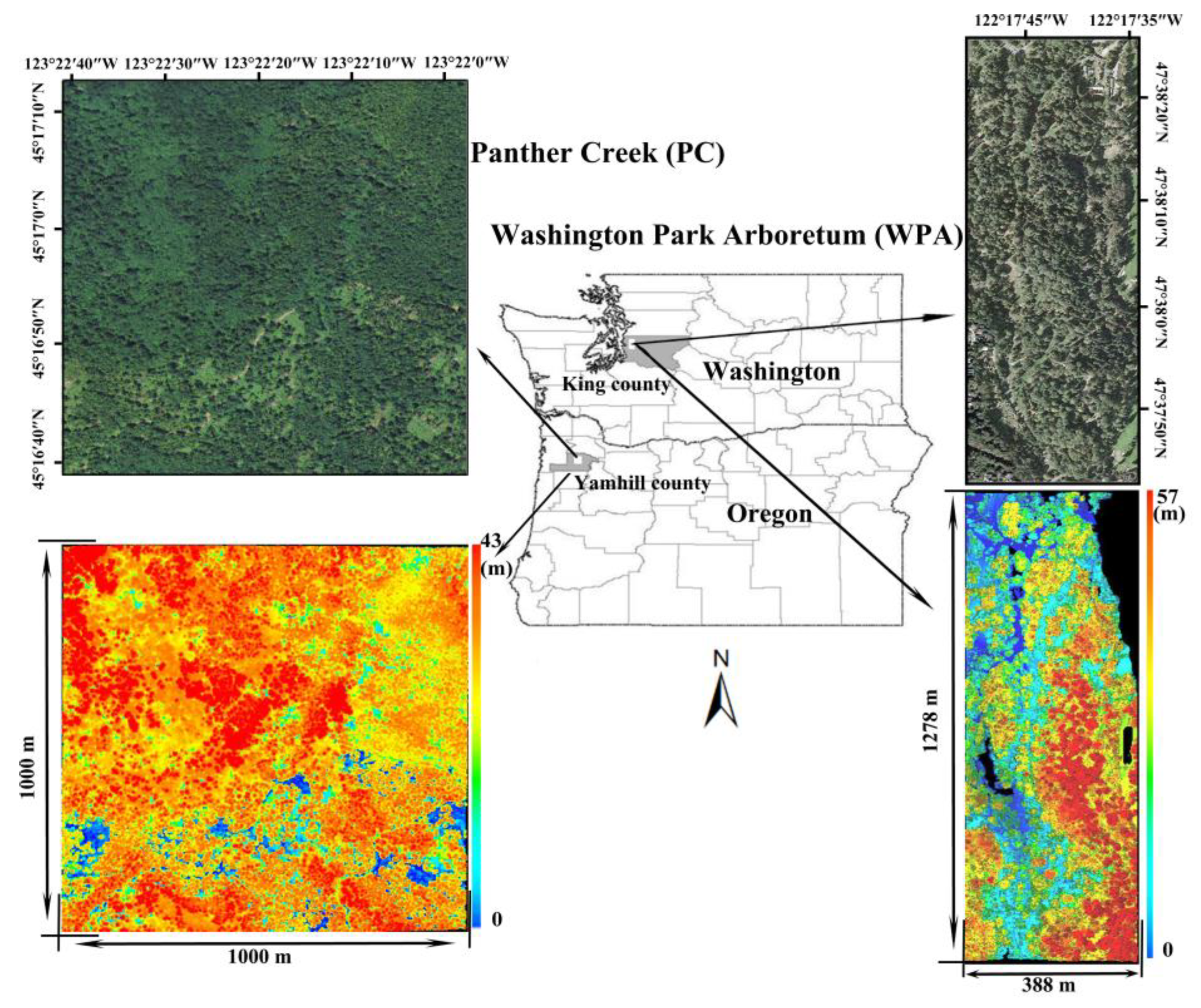
In this study, we first derived the tree locations and crown size information for two distinct urban heterogeneous and natural homogeneous forest stands based on the ALS data. Then, the point pair correlation function was used to identify the tree spatial distribution patterns. For each category, we approximated them using appropriate statistical models and determined their unknown parameters based on the ALS-based metrics. Finally, ALS-determined statistical models were validated using the Monte-Carlo simulation method. The flowchart of the current study was shown as follows (Figure 1):

2.1. Study Sites

Two study sites are selected in this study to test the performances of the proposed ALS-based approach in characterizing tree spatial distribution patterns at the landscape level. The first one locates in the Washington Park Arboretum (WPA), which is a well-managed urban forest. It is at the south of the University of Washington campus in Seattle, Washington, U.S.A. The dominant tree species of the WPA are douglas fir (Pseudotsuga menziesii), western hemlock (Tsuga heterophylla), western redcedar (Thuja plicata), big-leaf maple (Acer macrophyllum), monkey puzzle (Araucaria araucana), southern magnolia (Magnolia grandiflora), and new mexican locust (Robinia neomexicana). The slope throughout the WPA site is less than 15% (Figure 2). The second study site is at the Panther Creek (PC) watershed, which is a natural but still managed forest on the east side of the coastal mountain of Oregon, USA. It is located 57 km southeast of Portland, Oregon, USA at 45°18′N, 123°21′W. The elevation of Panther Creek watershed ranges from 100 m to 700 m. The douglas fir (Pseudotsuga menziesii), western hemlock (Tsuga heterophylla), western redcedar (Thuja plicata), and big-leaf maple (Acer macrophyllum) are dominant tree species. The spatial patterns at these two locations, due to the management practices and natural processes, are expected to be distinguishable and capture a wide range of tree spatial distribution patterns.

2.2. Datasets

• Aerial laser scanning data (ALS)

The airborne lidar data for the WPA site were acquired using a Riegl LMS-Q560 laser scanner (Riegl, Co. Ltd. Horn, Austria). The coverage was collected at an average elevation of 279 m and flight height was about 310 m on average. The scan angle of the laser scanner ranged from −30° to 30° from nadir. This ALS flight setting resulted in a discrete point dataset containing five returns per pulse and more than ten pulses per square meter.

In the PC site, the laser sensor Leica ALS80 (Leica Geosystems AG, Heerbrugg, Switzerland) mounted in an aircraft with a frequency of 394.8 kHz emitted a single laser pulse and view field of 30° at the flight height of 1400 m. Finally, it yielded a 3-D lidar data with an average density of greater than eight pulses per square meter over terrestrial surfaces. The average point densities in WPA and PC sites are 26 points/m² and 15 points/m², respectively.

• Validation data

To validate tree crown segmentation result and applicability of ALS-determined statistical models, we set up four squared forest plots in the WPA site, including a high-density coniferous plot (i.e., WPA-HC), a medium-density coniferous plot (i.e., WPA-MC), and low-density coniferous and mixed forest plots (i.e., WPA-LC and WPA-LM) with a side length of 100 m. Furthermore, two squared forest plots with the side length of 100 m in the PC site were also selected, including one high-density coniferous plot (i.e., PC-HC) and a medium-density coniferous forest plot (i.e., PC-MC). In the six forest plots, we visually identified treetop points and obtained total tree numbers and their locations from ALS point cloud data. By doing this, forest plots were divided into high- (>100 trees), medium- (≥80 trees and ≤ 100 trees), and low-densities (<80 trees) groups. The crown diameters were measured in crossed directions (North−South and East−West) for each tree crown in ALS-based forest data. Moreover, we identified forest types visually using aerial photographs with a spatial resolution of 0.3 m. More detailed information about the forest plots is summarized in

Table 1. Characteristics of forest plots in both natural and modeled forest sites.

Plot Type	Plot ID	Density	Tree #	Forest Type	Crown Radii (m)
					Max.	Min.	Average
Natural forest plots	WPA-HC	High	159	Conifer	7.26	1.62	3.72
	WPA-MC	Medium	95	Conifer	11.78	2.80	6.28
	WPA-LC	Low	75	Conifer	9.50	2.15	5.41
	WPA-LM	Low	66	Mixed	12.27	2.45	7.23
	PC-HC	High	150	Conifer	6.60	1.80	4.15
	PC-MC	Medium	92	Conifer	7.50	2.00	4.90
Modeled forest plots	Plot-1	Low	79	Conifer	3.81	3.81	3.81
	Plot-2	High	110	Conifer	3.81	3.81	3.81
	Plot-3	Low	79	Conifer	3.81	3.81	3.81
	Plot-4	High	105	Conifer	3.81	3.81	3.81
	Plot-5	Low	79	Conifer	3.81	3.81	3.81
	Plot-6	Medium	95	Conifer	3.81	3.81	3.81

.

• Modeled data

To illustrate the significant effects of tree spatial distribution patterns on estimating the probabilities of viewing the ground surface in a forest scene, we modeled six square forest plots with the side length of 100 m and identical individual tree ALS point cloud data (Table 1). We first simulated three different tree spatial distribution patterns (i.e., Random, Clustered, and Regular) in the R programming environment [44], then explored the probabilities of viewing the ground surface area from various directions. Moreover, each spatial distribution pattern was parameterized using two different sets of parameters.

2.3. ALS-Based Tree Crown Segmentation

We obtained the locations and crown sizes of each tree using the previously published ALS segmentation algorithm [41]. The spacing threshold and search radius are two primary parameters in the algorithm. To overcome the over- or under segmentation issue, we developed a “point cloud slicing-based tree verification” method to achieve a better segmentation result. In this study, we used the treetop point as tree location due to the inability to capture stem location using aerial remotely sensed data.

For the point cloud data of each segmented tree, we extracted six sliced planes with a thickness of 0.2 m in two different ways horizontally and vertically, respectively. The six slicing planes located at the 15%, 30%, 45%, 60%, 75%, and 90% heights (i.e., horizontal slicing) or distances along the X- or Y- axis (i.e., vertical slicing) of the segmented individual tree points. We computed the standard deviations of the X- and Y- coordinates (i.e., horizontal slicing), or X- and Z-, or Y- and Z- coordinates (i.e., vertical slicing) of the six center points from six sliced plane using the Equation (1):

$$\sigma =\sqrt{\frac{{\displaystyle \sum _{i=1}^{i=6}{(x_i-\overline{x})}^2}}{n-1}}$$

(1)

σ is the standard deviation; x_i is the value of coordinate (X-, Y-, or Z-) of the ith point in the six center points; $\overline{x}$ is the mean value of the coordinates of six center points. The points of an individual tree were labeled as a mis-segmented tree crown if the deviation of horizontal slicing was beyond 0.4 m. We determined the threshold as 0.4 m based on the distance deviations between treetop and bottom points in the case of a horizontal slicing way. As for the vertical slicing way, the threshold was set as 0.8 m, the one half of the minimum tree crown size by assuming tree crowns are symmetrical. By finishing the iteration process, we obtained the final results of the treetop location, crown diameter, and tree height at the individual tree level.

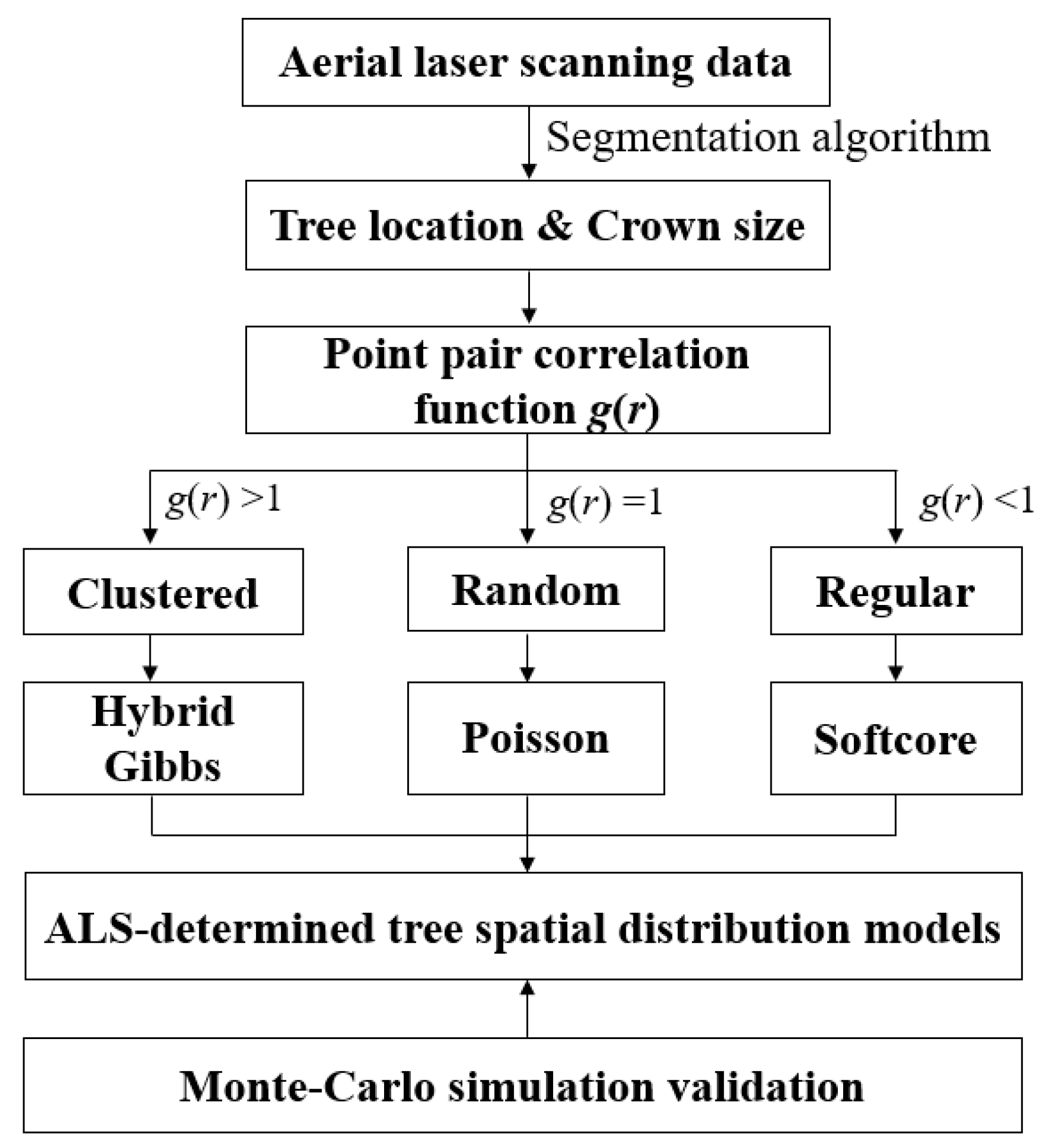
2.4. Tree Spatial Distribution Pattern Identification

The point pair correlation function (i.e., g(r) function) is a second-order summary statistic function determining the types of tree spatial distribution patterns (i.e., random, clustered, or regular) for a given point set [17,45]. The g(r) function is calculated based on the number of point pairs for a given arbitrary point within a distance of r [45]. It is proportional to the first-order derivative of Ripley’s K(r) function [46] concerning r:

$$g(r)=K’(r)/2\pi r$$

(2)

It contains the same statistical information as the K(r) function but the non-cumulative effect of K(r) function [47]. (1) Random distribution: if g(r) is constant and equal to one (i.e., g(r) = 1), it means that the location of any point is completely independent of the other point locations. It belongs to a completely random process (CSR) [48]; (2) Clustered distribution: if values of g(r) are greater than one (i.e., g(r) > 1), this suggests a clustering process caused by the aggregation effects of points; (3) Regular distribution: if values of g(r) are smaller than one (i.e., g(r) < 1). It indicates that the spatial distribution patterns of points tend to a regular pattern. It should be noted that there is a “virtual aggregation” phenomenon [17] in a forested area with patches of non-forest (i.e., human activities or deforestation) land at the landscape or region scales. In this case, the g(r) function suggests a clustered tree spatial distribution pattern across all spatial scales [17], and it is necessary to remove the non-forest areas to determine tree spatial distribution patterns.

To analyze the visual- and ALS-based g(r) function curves effectively, we computed the normalized g(r)_norm function as

$$g{(r)}_{norm}=\frac{g(r)-(G_{max}(r)+G_{min}(r))/2}{(G_{max}(r)-G_{min}(r))/2}$$

(3)

where g(r)_norm is the normalized value of g(r) function ranging from −1 to 1; G_max(r) and G_min(r) represent the simulation envelopes obtained as the 5th highest and lowest values after 999 simulations using the Monte Carlo simulation method [49]. This normalization procedure allows us comparing different envelope lines more efficiently.

2.5. ALS-Based Statistical Model Parameters Determination

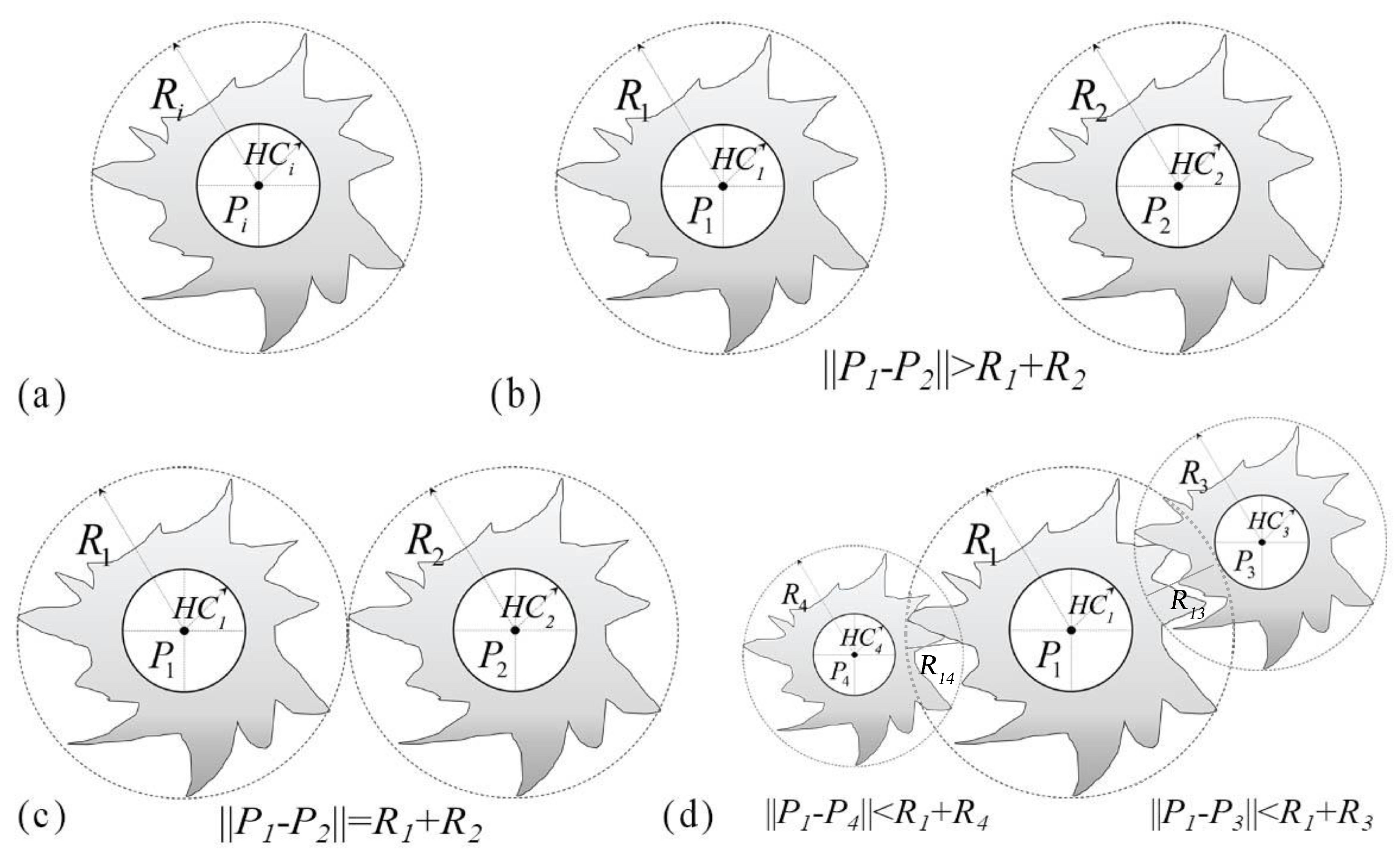
2.5.1. Tree Crown Competitive Effects Characterization

1. Individual tree crown model

To characterize the competitive effects [50] among tree crowns quantitatively, we proposed a new individual tree crown model. In this model, a tree crown was represented using two annulus circles with treetop points as the center point (i.e., P_i). The radii of two circles were HC_i and R_i, respectively (Figure 3a). The “hard-core” (i.e., inner circle) was a circular area of individual tree crown where no parts of other trees existed, while the “buffer region” (i.e., outer annulus circle) area might have overlapped parts between tree crowns. In the current study, we used the hard-core radius to describe the competitive effects among tree crowns: the larger hard-core radius, the more substantial competitive effect.

According to relative spatial locations among tree crowns, the interactions among tree crowns are classified into three categories: (a) separated tree crowns—two tree crowns (i.e., Tree-1 and Tree-2) with the treetop points P₁ and P₂, hard-core radii and buffer circle as HC₁ and HC₂, R₁ and R₂, respectively (Figure 3b). These are apart from each other when the distance between two treetop points is larger than the sum of radii of two tree crowns (i.e.,‖P₁ − P₂‖> R₁ + R₂); (b) tangent tree crowns—two tree crowns may be adjacent to each other (i.e., they share a tangent line) when the distance between two treetop points is equal to the sum of the radii of two buffer circles (i.e.,‖P₁ − P₂‖= R₁ + R₂, (Figure 3c); (c) overlapped tree crowns—two or more overlapped tree crowns within the tree crown “buffer regions” based on the geometric model of tree crowns (Figure 3d). For example, Tree-1 is overlapped in the buffer region by Tree-3 and Tree-4 whose treetop points and buffer regions radii are P₃, P₄, and R₃, R₄, respectively. The distances between every two treetop points are smaller than the sum of any two crown radii (i.e., ‖P₁ − P₄‖ < R₁ + R₄ and‖P₁ − P₃‖ < R₁ + R₃).

2. Hard-core radius determination

Determining the “hard-core” radius (HC_i) is a prerequisite to quantify the competitive effects among tree crowns using the hybrid-Gibbs model. In the current study, we obtained the hard-core radius of a forest plot using the proposed individual tree crown model. For an individual tree, it may be overlapped with multiple tree crowns. In the case of two tree crowns, we computed the hard-core radius of the i-th tree crown overlapped with the j-th tree crown by assuming that the hard-core radius of a tree crown was proportional to their crown sizes as

$$H{C}_{ij}=R_i-R_{ij}\cdot \frac{R_j^{}}{R_i^{}+R_j^{}}$$

(4)

where HC_ij is the estimated hard-core radius when the i-th tree crown overlapped with the j-th tree crown; R_i and R_j are the radii of the i-th and j-th tree crowns; R_ij is the line segment between the treetop points of the i-th and j-th tree crowns falling in the “buffer” regions and computed as

$$R_{ij}=(R_i+R_j)-\Vert P_i-P_j\Vert$$

(5)

If the target tree (i.e., the i-th tree) was overlapped by two other tree crowns (i.e., j-th and k-th tree crowns), we computed the hard-core radius of the i-th tree (i.e., HC_i) by averaging the estimated hard-core radii (i.e., HC_ij and HC_ik). For example, we first computed the overlapping distances (i.e., R₁₃ and R₁₄) based on Equation (5), and obtained the estimated hard-core radii (i.e., HC₁₃ and HC₁₄) for Tree-1 concerning Tree-3 and Tree-4 using Equation (4) (Figure 3d). The hard-core radius of Tree-1 was computed as the average values of HC₁₃ and HC₁₄. We used the averaged hard-core radii for all trees as the hard-core for the whole forest plot.

2.5.2. Three Different Tree Spatial Distribution Patterns

1. Random distribution:

We approximated a random tree distribution pattern using the simplest and well-accepted Poisson model [11,12,51] and computed as

$$P(y)=\frac{e^{-\lambda }{\lambda }^y}{y!}$$

(6)

where 𝜆 is the average tree number per unit area; P(y) is the probability of finding y trees in the sample area. The unknown parameter 𝜆 could be determined using the ALS-based metrics.

2. Regular distribution:

We used the “soft-core point process model” to approximate a regular tree spatial distribution pattern. Compared to hard-core point processes, the interaction of points in the soft-core point process is smoothly decreasing with distance increasing. It is an essential point process for biology because there is rarely an abruptly ending for the interactions between points [52]. The “soft-core” model of a regular distribution point set x = {x₁, x₂, … x_n} could be computed as

$$P(x)={\beta }^n\exp \{-{\displaystyle \sum _{i<j}{(\frac{\sigma }{\parallel x_i-x_j\parallel })}^{2/\kappa }}\}$$

(7)

where β is a contributing factor of each point to the global point process; σ controls the distance at which the interactions occur and is a positive real number. The larger values, the stronger interactions; κ indicates the strength of interactions between a point pair, and it is dimensionless variables ranging from 0 to 1; ‖x_{i −} x_j‖ is the distance between the two points. β is computed using the maximum likelihood estimator method [53], κ and σ are estimated using the maximum profile pseudolikelihood algorithm [54] using the ALS-based tree locations.

3. Clustered distribution:

The Neyman type-A and hybrid Gibbs models are the two most commonly used statistical models to approximate clustered tree spatial distribution patterns [11,31]. For comparison purposes, we have analyzed these two models in the current study. In a Neyman type-A model, there are “parent” (i.e., center points of every group) and “offspring” points (i.e., all non-parent points). If there are i trees in the given j groups within the quadrat, the probability of having i trees in the given j groups can be determined using these double-Poisson point processes and computed as

$$P(i;m_1;m_2)=\frac{m_2^i}{e^{m_1}i!}{\displaystyle \sum _{j=1}^{\infty }\frac{{[m_1{e}^{-m_2}]}^j}{j!}}\cdot j^i$$

(8)

where m₁ is the mean number of groups in the quadrat, and m₂ is the mean size of the groups. In the process of model realizing, m₁ is approximated by the density of group centers (𝜆_N), and m₂ is represented by group radius (r_N) together with the mean number of points per group (m_N). The minimum contrast estimation method [55] could be used to determine the unknown parameters (𝜆_N, r_N, m_N) of the Neyman-A model using ALS-based tree locations. However, the Neyman-A model only treats tree crowns as an individual point without considering the crown size and their interactions. Hybrid Gibbs model can approximate spatial distribution patterns under different scales using various pairwise interaction functions. Then we built a hybrid Gibbs model by combining the “hard-core” and “Geyer” point processes [56] to better characterize clustered tree spatial distribution patterns by incorporating the competitive effects among tree crowns (i.e., hard-core radius). The probability density of a point sets based on the newly constructed hybrid Gibbs model can be computed as

$$P(x)={\beta }^n{\displaystyle \prod _{i=1}^{n}H(r)}\cdot {\gamma }^{\min (s,t(x_i,x\backslash x_i,r_g))}$$

(9)

where r is the distance between a point pair; H(r) is the probability density of the “hard-core” point process model; x is an unordered point set x ={x₁, x₂, … x_n}; n is the total number of points in the point set (n ≥ 0); s is the saturation threshold to limit the number of distinct unordered points that are closer than r units apart; t(x_i, x\x_i, r_g) is the number of neighbors of x_i in point set x; r_g represent the interaction ranges, and γ controls the strength of the repulsion (i.e., γ < 1) and attraction (i.e., γ > 1) interactions between points in the process. The parameter β controls the density of a point process; for a given γ, the density of point process increases as β increasing. The value of β equals the density of the Poisson process when γ = 1. The values of s and γ can be estimated using the maximum profile pseudolikelihood algorithm based on ALS-based tree locations [54], β can be obtained using the maximum likelihood estimator method [53]. We determined the hard-core radius using the method described in Section 2.5.1 based on ALS-based tree locations and crown sizes. The values of H(r) and P(x) equal 0 when r is smaller than 2×HC, suggesting that no point is generated. H(r) equals 1 when r is greater than the 2×HC. In this case, the hybrid Gibbs model will be equivalent to the Geyer model. We can rewrite Equation (9) as

$$P(x)={\beta }^n{\displaystyle \prod _{i=1}^n{\gamma }^{\min (s,t(x_i,x\backslash x_i,r_g))}}$$

(10)

By doing this, we can determine the unknown parameters of statistical models used for approximating various tree spatial distribution patterns quantitatively.

2.6. ALS-Determined Tree Spatial Distribution Models Validation

To test the suitability of the ALS-determined statistical model for a given forest plot, we compared the 95% confidence intervals simulated from the ALS-determined statistical model with the “reference g(r) function curve.” The reference g(r) function curve was produced based on the tree locations determined through visual interpretation. We generated the envelope lines through repeated random sampling (i.e., typically 999 times) based on the ALS-determined statistical models using the Monte-Carlo simulation method [49]. If the reference g(r) function curve fell into the envelope lines generated using a specific ALS-determined statistical model completely, the corresponding statistical model will be identified as a qualified model to approximate tree spatial distribution patterns.

2.7. Sensitivity Analysis

We compared the ALS-based tree locations and crown sizes with the ones obtained from the visual interpretation method by changing the spacing thresholds and search radii from 1 m to 5 m with the step of 1 m for the natural forest plots. Moreover, to investigate the effects of overlapping distances on the accuracy of tree crown segmentation, we conducted a numeric simulation experiment by changing the overlapping distances from 1 m to 4 m with the step of 1m in three different tree species configurations (i.e., conifer + conifer, broadleaf + broadleaf, conifer + broadleaf). In the forest plot WPA-HC, by changing the radii of hard-core from 1.4 m to 2.0 m with the step of 0.1 m, we explored the effects of hard-core on tree spatial distribution patterns.

Moreover, to illustrate the importance of tree spatial distribution patterns on simulating forest canopy directional reflectance using the existing method [57], we computed the probabilities of viewing the ground surface from various directions in principle plane. The azimuthal and zenith angles of sun were set as 90°and 30°, while the viewing azimuthal (VA) and viewing zenith angle (VZ) of observations directions were set as 90° and 0°, 90° and 30°, 90° and 60°, 270° and 30°, 270° and 60°, respectively.

3. Results

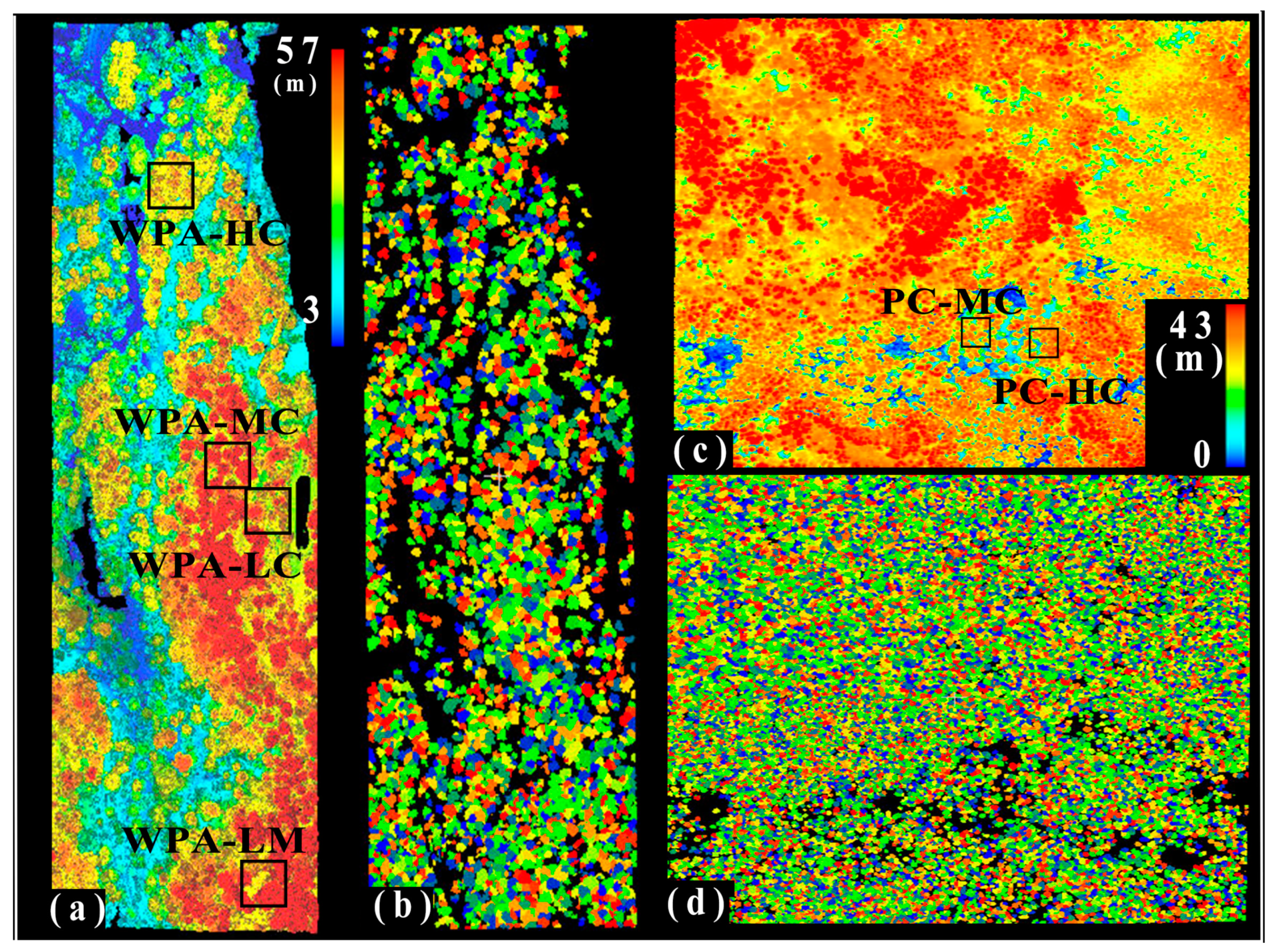
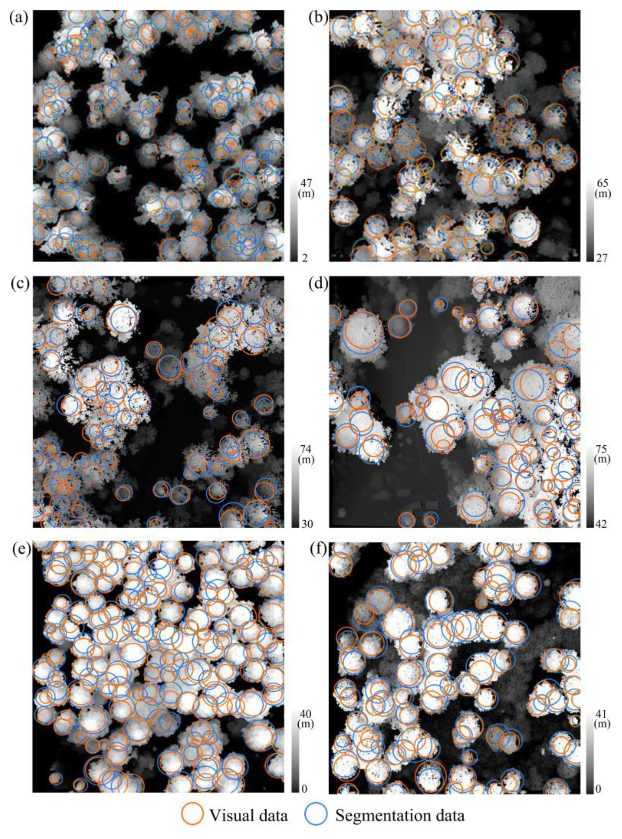
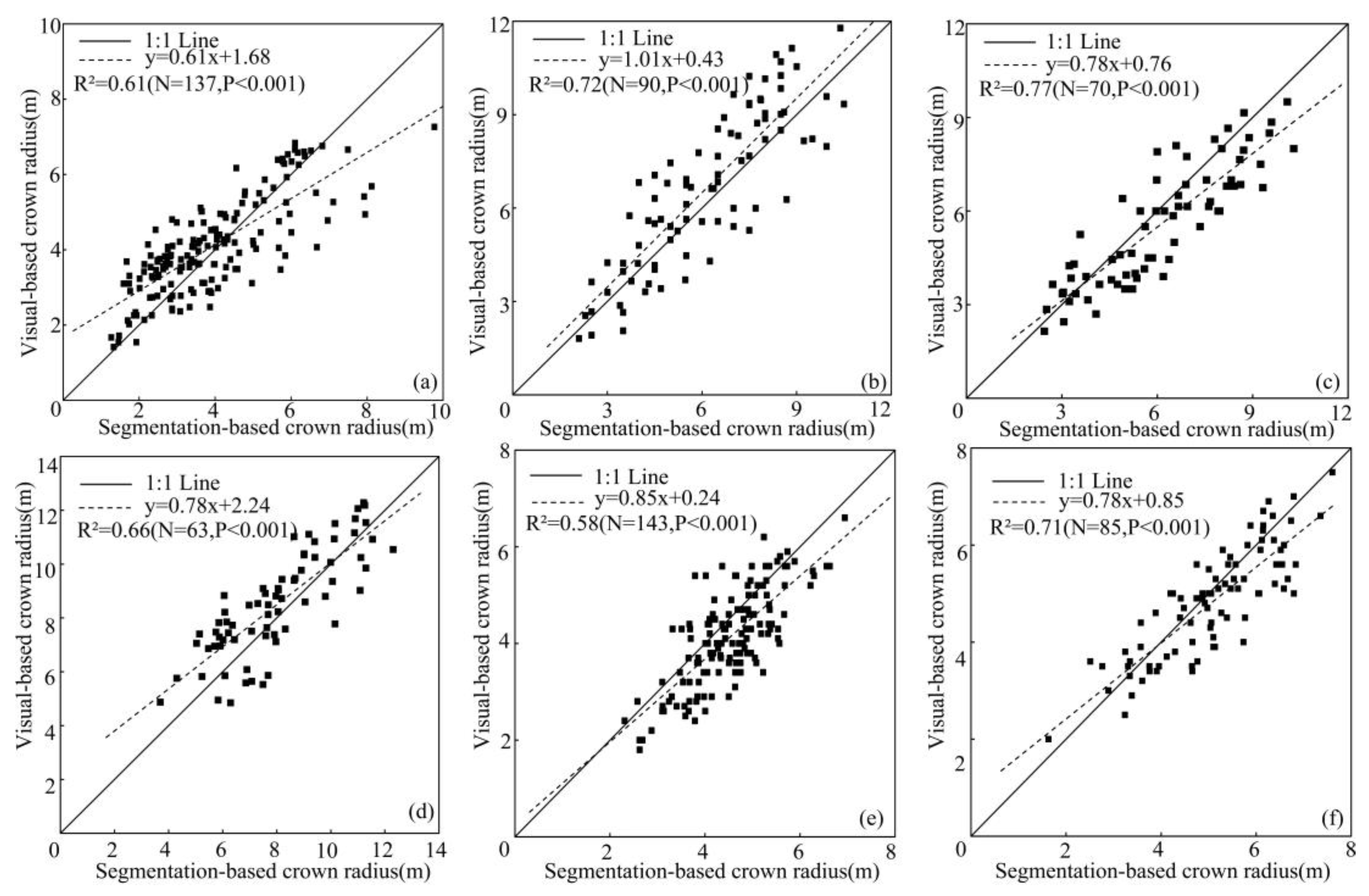
3.1. ALS-Based Tree Locations and Crown Sizes

After applying the ALS-based tree segmentation algorithm, raw point cloud data were grouped into individual trees represented by different colors at in both WPA and PC sites. Figure 4a, c shows the original ALS data for the whole WPA and PC sites. The individual tree segmentation results have been obtained using the method described in Section 2.3 for WPA (Figure 4b) and PC sites (Figure 4d).

We obtained the treetop location, tree number, crown radius, tree height, and stem density from ALS forest data. Based on the ALS-based treetop points, we approximated each tree crown as a geometrical circle and compared the ALS-based tree crowns with the visual-based results for forest plots WPA-HC (Figure 5a), WPA-MC (Figure 5b), WPA-LC (Figure 5c), WPA-LM (Figure 5d), PC-HC (Figure 5e), and PC-MC (Figure 5f), respectively.

By comparing the visual- and ALS-based tree crown radii (Figure 6), we found that the values of the correlation coefficient increased from 0.61 to 0.77 as forest densities decreased in urban forest plots WPA-HC, WPA-MC, and WPA-LC (Figure 6a–c). Moreover, the mixed forest types were lower the value of R² in the low-density forest plots WPA-LC (i.e., 0.77) and WPA-LM (i.e., 0.66) (Figure 6c,d). As for the natural forest stand, an increasing trend in R² was observed for the natural forest plots PC-HC (i.e., 0.58) and PC-MC (i.e., 0.71). Although, there were similar R² values between the ALS- and visual-based tree crown radii in forest plots WPA-MC (i.e., 0.72) and PC-MC (i.e., 0.71), apparent RMSE differences were observed in WPA-MC (i.e., 1.39 m) and PC-MC (i.e., 0.85 m). Different forest vertical structures might explain this discrepancy in these two forest sites. Since the WPA site is a mixed urban forest with well-managed practices, it has an apparent adjacent configuration of over- and under-stories with different tree species and crown shapes. However, in the PC natural coniferous forest, there are relatively fewer understory crowns. As shown in

Table 2. Characteristics of ALS-based individual trees for forest plots in both WPA and PC sites.

Plot ID	Density	Tree #	Tree Detection Rate	Tree Location RMSE (m)	Crown Radii (m)
					Range (Max.–Min.)	Average	RMSE
WPA-HC	High	137	86%	2.51	8.770–1.26	3.38	1.45
WPA-MC	Medium	90	95%	2.20	10.50–2.10	6.13	1.39
WPA-LC	Low	70	93%	1.46	10.31–2.45	6.09	1.16
WPA-LM	Low	63	95%	1.47	12.28–2.50	6.83	1.50
PC-HC	High	143	95%	1.72	6.94–2.30	4.53	1.05
PC-MC	Medium	85	92%	1.67	7.75–1.63	5.08	0.85

, it was found that in the urban forest canopies, the RMSE of ALS-based tree locations increased from 1.46 m to 2.51 m as the forest densities increasing. For the low-density forest plot, both the coniferous (i.e., WPA-LC) and mixed (i.e., WPA-LM) forest plots have small RMSEs of 1.46 m and 1.47 m, respectively. In the natural forest canopies, both high- and medium-density forest plots achieved small RMSE values for ALS-based tree locations due to the well-separated tree crowns in a natural coniferous forest environment. The mixed tree species and complicated vertical structure in the WPA site might increase the overlapping between tree crowns and further introduce errors into the estimation of tree locations.

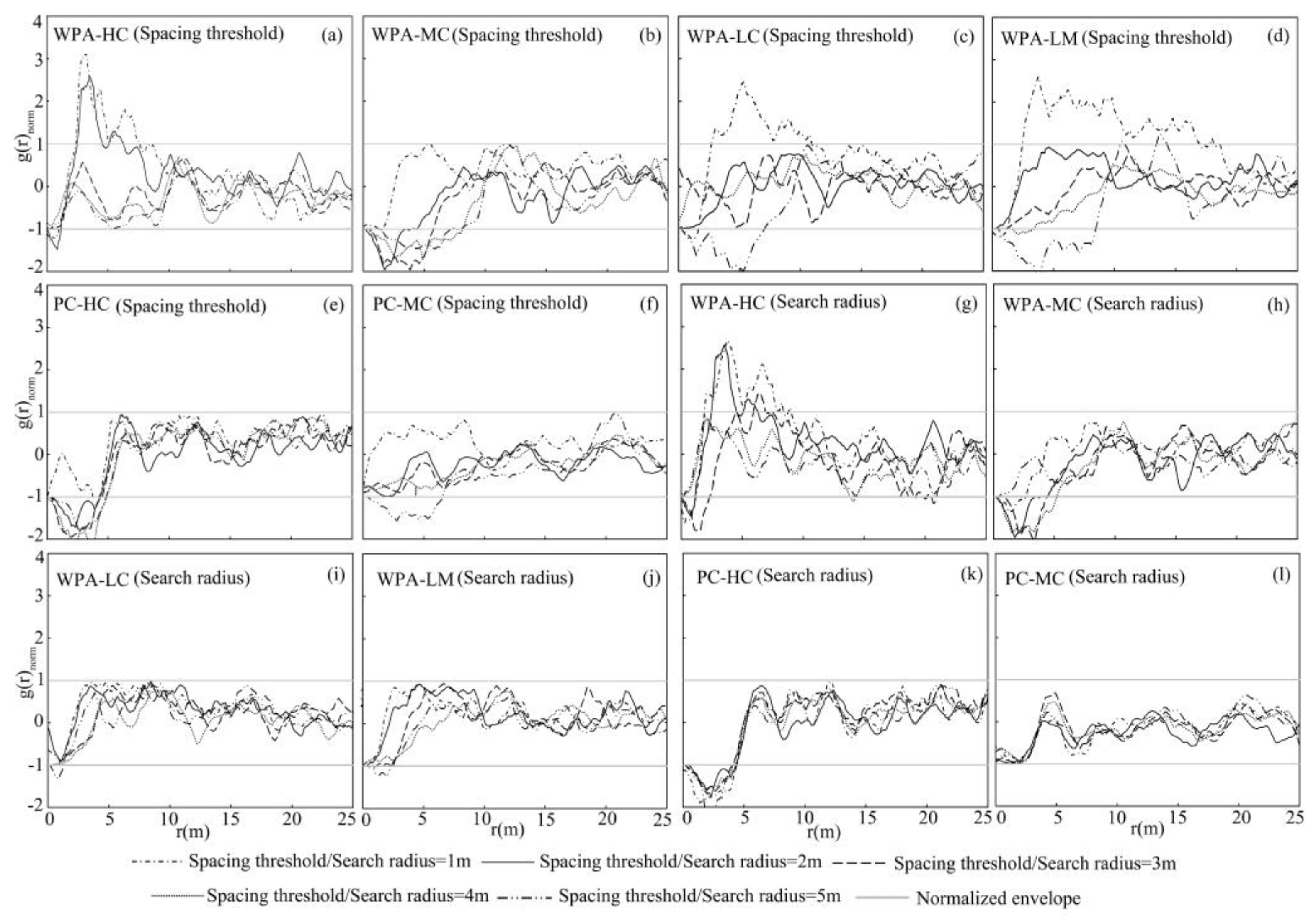
3.2. ALS-Based Tree Spatial Distribution Patterns

Based on the ALS- and visual-based tree locations, we obtained two normalized g(r) functions for six forest plots in both WPA and PC sites (Figure 7). Overall, the ALS-based g(r)_norm function curves have similar variation patterns with the visual-based ones for all forest plots. In forest plot WPA-HC (Figure 7a), the curves of both ALS- and visual-based g(r)_norm functions were out of the normalized envelope lines. The ALS-based values of g(r)_norm function exhibited different patterns (i.e., 1 < g(r)_norm when 2.94 m < r < 6.65 m or g(r)_norm < 1 when r < 1.81 m) at different ranges, indicating a mixed point spatial distribution at different spatial scales. However, the g(r)_norm function of visual-based tree locations was smaller than 1 when r < 1.28 m, and larger than 1 when 1.96 m < r < 3.82 m. The tree spatial distribution pattern in WPA-HC was classified as a clustered distribution incorporated with competitive effects between tree crowns. In this case, a single scale statistical model, such as a Neyman-A model, is not enough for comprehensively characterizing the tree spatial distribution patterns. Thus, a generic and more sophisticated model, such as the hybrid Gibbs model, should be implemented instead.

Regarding the forest plot WPA-MC (Figure 7b), only part of g(r)_norm function stayed within the normalized 95% confidence intervals when the distance between pair points r was beyond 6.5 m. The visual- and ALS-based g(r)_norm functions were out of the range of normalized envelope lines when distance r was less than 5.7 m and 6.5 m, respectively, indicating that the tree spatial distribution pattern was regular. Therefore, the soft-core point process model would be the optimum one to approximate the tree spatial distribution patterns in this case. As for forest plots WPA-LC and WPA-LM (Figure 7c,d), the ALS-and visual-based g(r)_norm functions fell well within the normalized 95% envelope lines (i.e., g(r)_norm = 1 and −1), suggesting that the trees within these forest plots exhibited a random distribution pattern. Accordingly, the Poisson model should be used to approximate its tree spatial distribution patterns.

In the PC site, the forest plots PC-HC (Figure 7e) and PC-MC (Figure 7f) have similar g(r)_norm function curves with the forest plots WPA-MC and WPA-LM, respectively. In the forest plot PC-HC, the visual- and ALS-based g(r)_norm functions were out of the normalized envelope lines when the r < 4.19 m and 5.02 m, respectively. The forest plots PC-HC and PC-MC were classified into regular and random distribution patterns. Thus, the soft-core point process model and the Poisson model were chosen to approximate the tree spatial distribution patterns.

For the whole study area of both WPA and PC sites, the mix of forest and non-forest made the ALS-based g(r) function curves deviated from the 95% confidence interval lines of the null model (i.e., CSR) (Figure 8a,c). Moreover, the extent of ALS-based g(r) function curves deviating from envelope lines in the WPA site was more significant than in the PC site because the WPA site is a well-managed urban forest with more non-forest area coverages. After masking out the non-forest land cover, we obtained a reasonable ALS-based g(r) function curves that partially fell into the envelope lines (Figure 8b,d). It was shown that the ALS-based g(r) were smaller than 1 when the r < 6.2 m and r < 7.1 m for WPA and PC sites, respectively. Therefore, the tree spatial distribution patterns in the WPA and PC sites were considered as regular distribution based on the criteria described in Section 2.4, and the soft-core point process model was used to model the tree spatial distribution pattern.

3.3. ALS-Determined Parameters of Tree Spatial Distribution Models

Once the tree spatial distribution pattern is determined, an appropriate empirical statistical model can be used to approximate the tree spatial distribution pattern. Based on the coordinates of trees and crown sizes, we obtained the unknown parameters of different statistical models for six natural forest plots in both WPA and PC sites (

Table 3. ALS-determined input parameters for the Poisson, soft-core, Neyman-A, and hybrid Gibbs models.

Statistical Models	Input Parameters	ALS-Based Values	Visual-Based Values
Hybrid Gibbs (WPA-HC)	Control factor of density (β)	0.007	0.009
	Hard-core distance (HC)	1.650	1.500
	Interaction radius (rg)	3.500	3.000
	Saturation threshold (S)	3.000	3.000
	Interaction parameter gamma (γ)	1.920	2.110
Neyman-A (WPA-HC)	Density of cluster centers(λN)	0.016	0.018
	Radius of the clusters (rN)	5.090	3.250
	Mean number of points per cluster (mN)	1.370	1.500
Poisson (WPA-LM/ WPA –LC/ PC-MC)	Density (λ)	0.006/ 0.007/ 0.008	0.006/ 0.007/ 0.009
Soft-core (WPA-MC/ PC-HC)	Interaction distance (σ)	5.450/ 4.450	4.500/ 3.700
	Control factor of interaction strength (κ)	0.500/ 0.400	0.390/ 0.320
	Control factor of density (β)	0.020/ 0.027	0.045/ 0.035

). For forest plot WPA-HC with clustered distribution pattern, three unknown parameters including 𝜆_N, r_N, and m_N were obtained for the Neyman-A model using ALS- (visual-) based data as 0.016 trees/m² (0.018 trees/m²), 5.09 m (3.25 m), and 1.37 (1.50), respectively. Moreover, parameters β, HC, r_g, γ and s of hybrid Gibbs model were determined as 0.007 (0.009), 1.65 (1.50) m, 3.5 (3.0) m, 1.92 (2.11), and 3 (3) based on the ALS- (visual-) based data, respectively. In terms of the regular distribution WPA-MC and PC-HC, the determined parameters (β, σ, and κ) for the soft-core point process models were 0.02 (0.045), 5.45 (4.50) and 0.50 (0.39) using the ALS- (visual-) based data for plot WPA-MC. In plot PC-HC, the ALS- and visual-based unknown parameters (β, σ, and κ) of the Soft-core point process model were 0.027 and 0.035, 4.45, and 3.70, 0.40 and 0.32, respectively. As for the plots WPA-LM, WPA-LC, and PC-MC were determined as random distribution, the ALS- and visual-based density (λ) parameters were the same as the ones of forest plots WPA-LM (0.006 trees/m²) and WPA-LC (0.007 tree/m²). Moreover, the ALS- and visual-based densities were 0.008 trees/m² and 0.009 trees/m² for forest plot PC-MC.

According to the methods described in Section 2.5, we determined the unknown parameters of the Soft-core point process models for the complete coverage in both WPA and PC sites based on the ALS-based metrics. The detected number of trees was 2745 and 7669 for WPA and PC sites, with the average crown radii as 5.49 m and 5.03 m, respectively. The determined unknown parameters including σ, κ, and β were 4.73 (6.52), 0.60 (0.75), and 0.10 (0.19) for WPA (PC) site (

Table 4. ALS-determined parameters of the soft-core point process model in both WPA and PC sites.

Sites	Coverage	Tree #	Crown Radii (m)		Model Type	Input Parameters
			Range (Min.–Max.)	Average		β	σ	κ
WPA	392 m × 1282 m	2745	1.26–11.30	5.49	soft-core	0.10	4.73	0.60
PC	1 km × 1 km	7669	2.56–10.37	5.03	soft-core	0.19	6.52	0.75

). Furthermore, for the whole study area of both WPA and PC sites, the ALS-based g(r) function completely fell into the envelope lines generated by the ALS determined soft-core point process model (Figure 8e,f).

In addition, we also determined the three parameters (i.e., β, κ, and σ) of modeled soft-core point process in the R programming environment as 0.013, 0.1, and 4.64 for forest Plot-1 and 0.025, 0.1 and 4.50 for forest Plot-2, respectively. The determined parameter of the Poisson point process for random distribution were 0.007 and 0.012 for modeled forest Plot-3 and Plot-4, respectively. In terms of the simulated clustered forest distribution pattern, the three unknown parameters (i.e., 𝜆_N, r_N, and m_N) were 0.002, 7.578, and 3.083 for forest Plot-5 and 0.002, 4.378, and 3.783 for Plot-6, respectively using the Neyman point process.

3.4. Validation of ALS-Determined Tree Spatial Distribution Models

To verify the applicability of the statistical models with determined parameters derived from ALS data we compared the visual-based g(r) function curves with the 95% envelope lines generated based on the ALS determined statistical models for six natural forest plots in both WPA and PC sites (Figure 9). It was found that a partial visual-based g(r) function curve was out of the envelope lines for forest plot WPA-HC (Figure 9a). The peak value of the ALS-based g(r) function shifted toward the right side, indicating that the tree spatial distribution pattern characterized by ALS data has less clustered strength. The corresponding larger r value showed that the clustering occurred at a larger spatial scale. This discrepancy might be attributed to the errors of individual tree segmentation result from the small tree crowns adjacent to the big tree crowns. The mis-segmentation will result in bigger ALS-based crown radius values. However, the visual-based g(r) function curves fall entirely into the envelope lines generated based on the ALS determined soft-core point process and Poisson model in forest plots WPA-MC (Figure 9b), WPA-LC (Figure 9c), WPA-LM (Figure 9d), PC-HC (Figure 9e), and PC-MC (Figure 9f). It indicated that appropriate statistical models with determined parameters derived from ALS data had been successfully applied to approximate the tree spatial distribution patterns.

As for the forest WPA-HC, we plotted the ALS- and visual-based g(r) function curves with the envelope lines generated based on the ALS determined Neyman-A model (Figure 9g). It was found that both ALS- and visual-based g(r) function curves did not fall into the envelope lines suggesting that the Neyman-A model could not approximate the tree spatial distribution. However, the envelope lines obtained based on the hybrid Gibbs model have similar variations with one produced by the visual-based measurements (Figure 9a). Then compared with the Neyman-A model, the hybrid Gibbs model was more effective at modeling the clustered tree spatial distribution.

4. Discussion

4.1. Tree Segmentation Accuracy Analysis

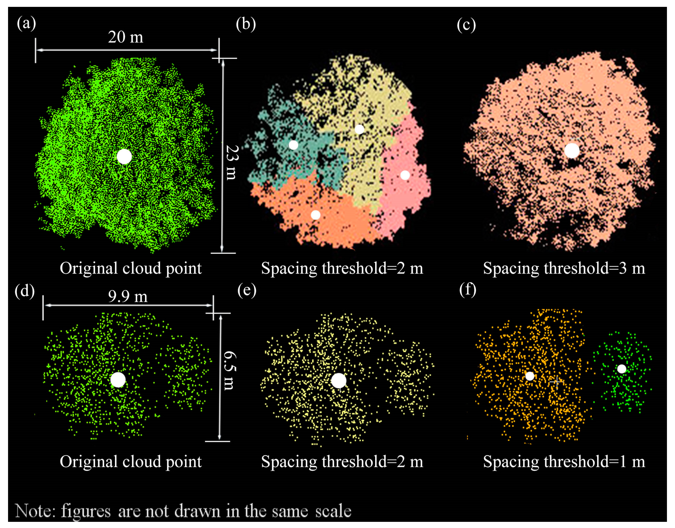
4.1.1. Spacing Threshold Effects

By conducting a sensitivity analysis of spacing thresholds on the normalized g(r)_norm functions, it was shown that the spacing threshold had obvious effects on ALS-based individual tree segmentation results (Figure 10a–f and Appendix A.

Table A1. Tree segmentation results using different spacing thresholds in both WPA and PC sites (Search radius = 2 m; shape index = 1.5; height threshold = 10 m;).

Plot ID	Observed Patterns	Observed Tree #	Spacing Threshold (m)	Segmented Tree #	Crown Radii (m)		Predicted Patterns
					Range (Min–Max.)	Average
WPA-HC	Clustered	159	1	252	1.03–6.79	2.96	Clustered
			2	137	1.26–8.77	3.38	Clustered
			3	110	2.30–10.71	5.92	Random
			4	89	2.35–11.32	7.72	Random
			5	77	2.50–12.06	8.67	Random
WPA-MC	Regular	95	1	130	1.59–7.79	3.37	Random
			2	90	2.10–10.50	6.13	Regular
			3	85	2.98–11.06	6.57	Regular
			4	67	2.69–11.17	7.55	Regular
			5	58	2.94–11.5	9.61	Regular
WPA-LC	Random	75	1	156	1.08–7.41	3.09	Clustered
			2	70	2.45–10.31	6.09	Random
			3	63	2.52–11.32	6.42	Random
			4	61	2.85–11.30	6.69	Random
			5	57	2.85–11.33	8.23	Regular
WPA-LM	Random	66	1	123	1.47–10.94	5.32	Clustered
			2	83	2.30–11.30	6.61	Random
			3	63	2.50–12.70	7.13	Random
			4	50	3.21–12.28	7.63	Regular
			5	47	4.70–12.53	7.96	Regular
PC-HC	Regular	150	1	171	1.61–6.65	3.70	Random
			2	143	2.32–6.94	4.53	Regular
			3	129	2.42–9.66	5.26	Regular
			4	106	3.11–10.05	5.85	Regular
			5	81	2.61–10.47	6.32	Regular
PC-MC	Random	92	1	120	1.38–7.32	3.65	Random
			2	85	1.63–7.75	5.08	Random
			3	83	2.64–10.12	6.56	Random
			4	72	2.98–10.47	7.15	Random
			5	60	2.86–10.72	7.55	Regular

). As the values of spacing thresholds increasing from 1 m to 5 m for six natural forest plots, the number of ALS-based segmented tree crowns decreased, and average tree crown radii increased regardless of the forest plots densities and types (Appendix A. Table A1). Moreover, with the changing spacing threshold, the predicted tree spatial distribution patterns were not constant with various numbers of the segmented tree. For example, in the plot WPA-HC, the tree number and average crown radii obtained using the visual-based measurements were 159 and 3.72 m, respectively. However, we obtained 252 trees and the crown sizes ranging from 1.03 m to 6.79 m, with an average value of 2.96 m, based on ALS data when the spacing threshold was 1 m.

Moreover, the predicted tree spatial distribution patterns were mixed when the spacing thresholds were 1 m or 2 m, which was consistent with the pattern produced by the visual-based measurements. However, the tree spatial distribution pattern in WPA-HC became random when the spacing thresholds were as 3 m, 4 m, or 5 m, respectively (Figure 10a). This variation might be explained by the fact that multiple aggregated trees have been identified as one bigger tree when the spacing threshold increased. Then, the selection of the spacing threshold is a key step in the ALS-based method for characterizing the tree spatial distribution patterns. By comparing the numbers of ALS- and visual-based tree crowns in all forest plots, it was found that the minimum tree crown radius was a good reference to set the appropriate spacing threshold. For example, the visual-based minimum tree crown radius (i.e., 1.62 m) in forest plot WPA-HC was similar to the optimum spacing threshold (i.e., 2 m). However, it is not efficient for the mixed forest plot because the appropriate spacing threshold is different for various crown shapes (Figure 11a,d) when applying the ALS-based tree segmentation algorithm. As shown in Figure 11, the broadleaf was segmented into four individual tree crowns, and the two coniferous crowns were delineated as one tree crown when the spacing threshold was set as 2 m (Figure 11b,e). When we set the spacing threshold as 3 m and 1 m, the broadleaf (Figure 11c) and coniferous (Figure 11f) crowns have been identified correctly, respectively. Considering the complexity of forest, we recommend the use of iterative tree crown segmentation method described in Section 2.3 to obtain tree locations and crown sizes information from ALS data, especially in landscape or region scales.

4.1.2. Search Radius Effects

The search radius has limited effects on the final accuracy of tree crown segmentation. By plotting the variations of normalized g(r)_norm functions with the search radii changing from 1 m to 5 m with the step of 1 m for six natural forest plots in both WPA and PC sites, it was found that similar variation patterns could be observed for all forest plots in both WPA and PC sites (Figure 10g–l). With the search radii increased from 1 m to 5 m, the number of segmented trees decreased, and average crown radii increased in general. For forest plots in the WPA site, as the search radius increasing, the predicted tree spatial distribution patterns changed accordingly since the search radius affected the result of tree crown segmentation. For example, in forest plot WPA-HC, the number of segmented trees was 189, 137, 129, 113, and 108 as the search radii increasing from 1m to 5 m with the step of 1 m. Furthermore, the average value of crown radii was 3.13 m, 3.38 m, 4.65 m, 6.1 m, and 7.21 m with an increasing search radius (Appendix A.

Table A2. Tree segmentation results using different search radii in both WPA and PC study sites (Spacing threshold = 2 m; shape index = 1.5; height threshold = 10 m;).

Plot ID	Observed Patterns	Observed Trees #	Searching Radius (m)	Segmented Trees #	Crown Radii (m)		Predicted Patterns
					Range (Min.–Max.)	Average
WPA-HC	Clustered	159	1	189	1.05–7.02	3.13	Clustered
			2	137	1.26–8.77	3.38	Clustered
			3	129	2.11–9.55	4.65	Clustered
			4	113	2.59–10.97	6.10	Random
			5	108	2.65–11.32	7.21	Random
WPA-MC	Regular	95	1	114	1.43–10.24	4.12	Regular
			2	90	2.10–10.50	6.13	Regular
			3	83	2.25–10.74	6.35	Regular
			4	78	2.26–11.60	6.79	Regular
			5	65	2.56–11.70	7.03	Random
WPA-LC	Random	75	1	115	1.13–9.44	3.85	Random
			2	70	2.45–10.31	6.09	Random
			3	62	2.46–11.32	6.31	Random
			4	59	2.49–11.33	6.33	Random
			5	45	2.59–11.33	6.96	Regular
WPA-LM	Random	66	1	113	1.05–11.30	5.79	Random
			2	63	2.50–12.30	6.61	Random
			3	59	2.64–11.50	6.65	Random
			4	57	2.53–11.33	6.87	Random
			5	44	4.70–12.53	7.12	Regular
PC-HC	Regular	150	1	160	1.51–8.65	4.54	Regular
			2	143	2.32–6.94	4.53	Regular
			3	140	2.22–8.65	4.89	Regular
			4	131	2.22–9.66	5.07	Regular
			5	128	2.32–9.87	5.23	Regular
PC-MC	Random	92	1	97	1.47–6.97	4.43	Random
			2	85	1.63–7.75	5.08	Random
			3	83	3.22–8.97	6.05	Random
			4	81	3.20–9.37	6.12	Random
			5	82	3.90–9.72	6.51	Random

). Moreover, when the search radii were beyond 4 m, the tree spatial distribution pattern shifted from clustered to random distribution (Figure 10g).

The natural forest plots showed constant distribution patterns such as regular and random forest plots PC-HC and PC-MC (Appendix A. Table A2). Furthermore, through comparing the ALS- and visual-based tree crown radius, the ALS-based tree crown sizes showed better performance in natural forest stands with small averaged standard deviation (i.e., 0.95) of crown sizes compared with the one (i.e., 1.38) in a well-managed urban forest. A thumb rule to determine the search radius was that the search radius should be less than the minimum crown diameter in the plot.

4.1.3. Effect of Overlap on Individual Tree Segmentation

The complexity of forest structure will affect the accuracy of tree crown segmentation. Forest stands with monodominant and separated tree crowns will achieve better accuracy and efficiency compared with the mixed forest with substantial overlapping between tree crowns. The overlapping effect makes it difficult to identify the boundaries of individual tree crowns accurately, especially in adjacent regions. As shown in

Table 5. Tree segmentation results for two individual trees with various tree crown overlapping distances.

Forest Type	Crown Overlap(m)	Crown Size (m) (Tree-1/Tree-2)	Point Number# (Tree-1/Tree-2)	Average Error Crown Size (m)	Average Error (Point Number)
Conifer + Conifer	0	8.03/8.03	2931/2931	0	0
	1.0	8.20/7.47	3086/2776	0.36	155
	1.5	8.10/7.54	3105/2757	0.28	174
	2.0	8.50/7.30	3306/2556	0.60	375
	2.5	8.96/6.85	3506/2356	1.05	575
	3.0	9.25/6.17	3525/2337	1.54	594
	3.5	9.18/5.72	3708/2404	1.73	652
	4.0	9.87/5.63	3757/2105	2.12	826
Conifer + Broadleaf	0	7.59/10.26	1863/6877	0	0
	1.0	7.07/10.62	1974/6766	0.44	111
	1.5	6.90/10.46	2049/6691	0.45	186
	2.0	7.02/10.14	2166/6574	0.35	303
	2.5	7.1/10.59	2319/6421	0.41	456
	3.0	7.49/11.86	2501/6239	0.85	638
	3.5	13.79/2.55	8127/613	6.95	6264
	4.0	12.87/0	8740/0	—	—
Broadleaf + Broadleaf	0	10.26/10.26	6876/6876	0	0
	1.0	9.58/10.09	6684/7068	0.42	192
	1.5	9.51/9.85	6664/7088	0.58	212
	2.0	9.51/9.88	6535/7217	0.57	341
	2.5	7.26/9.35	5217/8535	1.95	1659
	3.0	7.18/9.26	5238/8514	2.04	1638
	3.5	7.38/12.66	5079/8673	2.64	1797
	4.0	7.02/12.85	5019/8733	2.92	1857

, the increasing overlapping distance between tree crowns affected the accuracy of tree crown segmentation results. In the case of two coniferous trees with the tree height and crown diameter of 24.50 m and 8.03 m, it showed that the number of classified points for Tree-1 changed from 2968 to 3757 by changing the overlapped distances between two tree crowns from 0.5 m to 4.0 m. However, the number of points for Tree-2 decreased from 2894 to 2105. Furthermore, the average error of segmented tree crown diameter changed from 0.22 m to 2.12 m as the overlapped distance increasing. It showed that the overlapping distance of tree crowns should be less than 2.50 m to achieve better accuracy (>80%) of tree crown segmentation in the coniferous forest in our work.

For two broad-leaved trees with tree height and crown diameter of 10.52 m and 10.26 m, the average error of segmented tree crowns increased from 0.42 m to 2.92 m as the overlapping distance increasing from 1 m to 4 m. For the overlapped crowns mixed with conifer (i.e., tree height is 15.38 m and crown diameter is 7.59 m) and broadleaf (i.e., tree height is 10.52 m, and crown diameters is 10.26 m), the average errors of tree crown segmentation increased from 0.44 m to 6.95 m with the overlapping distance increased from 1 m to 3.5 m. It showed that the overlapping range of tree crowns should be less than 2 m to achieve higher accuracy (80%) of tree crown segmentation in the mixed forest in our work. However, it should be noted that the reasonable overlap rate varied with tree species, crown shape, crown size, relative tree height difference, and canopy cover. In addition, the comprehensiveness of the acquired forest point cloud data greatly affects the accuracy of tree crown delineation. For example, the shadow effects resulted from the tall tree might prevent the penetration of laser beams from capturing the crowns of short trees. This shadow effect could be improved by the cross-direction method or increasing the density of the flight path.

In addition, we compared our segmentation result with the ones obtained from the method proposed by Silva et al. (2016) using liDR package in the R programming environment [58,59]. It was shown that the liDR-based method tended to over-segment. The segmented tree number of six forest plot (i.e., WPA-HC, WPA-MC, WPA-LC, WPA-LM, PC-HC, and PC-MC) were 167, 118, 87, 78, 167, and 118, respectively. Moreover, the RMSEs between the visual- and liDR-based tree crown radii for six forest plots were 1.83 m, 1.78 m, 1.65 m, 2.10 m, 1.42 m, and 1.25 m, respectively. The RMSE of tree location were 2.39 m, 1.92 m, 1.67 m, 1.79 m, 1.59 m, and 1.52 m, respectively.

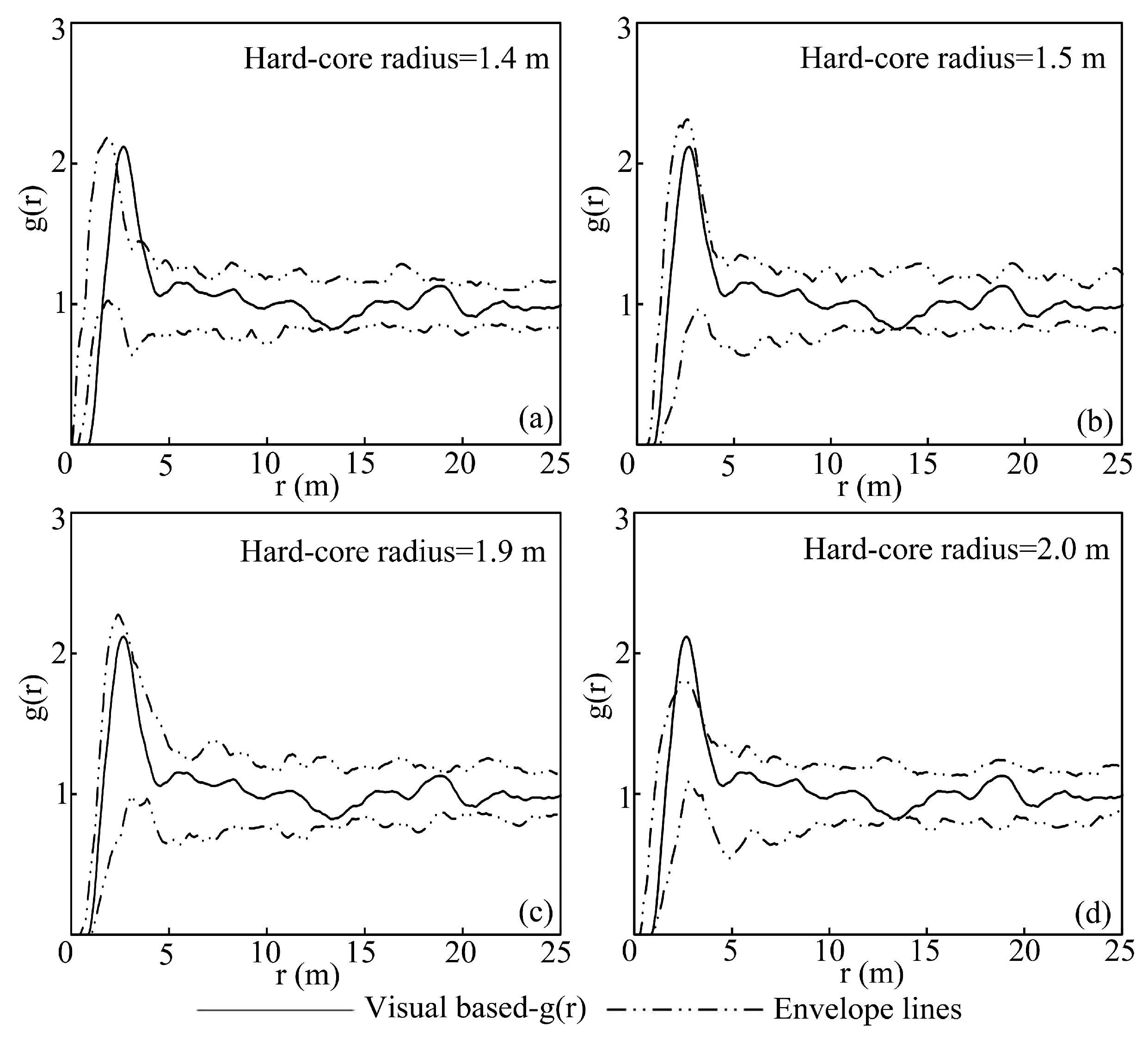
4.2. Effect of the Hard-Core Radius on Tree Spatial Distribution Pattern

The hard-core radii of individual tree crown within a certain range, which vary with tree species, crown sizes, and environmental conditions, usually has relatively stable effects on the tree spatial distribution pattern. Taking the forest plot WPA-HC for example, we compared the visual-based g(r) function curves with the envelope lines of the hybrid Gibbs models parameterized using visual-based hard-core radii in forest plot WPA-HC (Figure 12). It was found that, overall, the visual-based g(r) function curves could well fall into the envelope lines generated based on the hybrid Gibbs model with the hard-core radii of 1.4 m, 1.5 m, 1.9 m, and 2.0 m. More specifically, when the hard-core radius was 1.4 m, the visual-based g(r) function curve was out of the range of envelope lines when the g(r) < 1 at the regular distribution scale and shifted toward the right of the envelope lines (Figure 12a). It might be attributed to the fact that the smaller hard-core radius (e.g., 1.4 m) used in the hybrid Gibbs model could not explain the true competitive effects denoted by a visual-based hard-core radius (i.e., 1.5 m) well. When the hard-core radii ranged from 1.5 m to 1.9 m, the g(r) function fell within the 95% envelope lines (Figure 12b,c). However, as shown in Figure 12d, the visual-based g(r) function curve was out of the envelope lines produced based on the hybrid Gibbs model parameterized with a larger hard-core radius (i.e., 2 m). It indicated that the hybrid Gibbs model with determined parameters might not be able to capture the aggregation effect among tree crowns in this case. Therefore, the hard-core radius for a given forest plot is not a fixed value, especially in cases with various tree species and crown sizes. The fact that different tree species and crown sizes may have different hard-core radii might explain the unstable radii of hard-core of a forest stand.

4.3. Spatial Variations of Tree Spatial Distribution Patterns

The tree spatial distribution patterns usually exhibited varying patterns with the changes in the spatial scales of the observation windows, especially in the forest with a clustered distribution. For example, the random distribution pattern could be found within the observation windows with a smaller size in the natural forest PC site (Figure 13b). As the size of the observation window increased to 135 m × 135 m, the spatial distribution pattern gradually shifted into regular patterns due to the competitive effects (Figure 13c). The distribution pattern became a clustered one in 500 m × 500 m observation window (Figure 13d). The variations of the distribution patterns with the changing of observation window sizes have been shown clearly in its g(r) function curves. Therefore, an appropriate observation window should be determined before exploring tree spatial distribution patterns according to the interest of the study. A larger observation window should be used if the primary interest is to investigate the effect of environmental factors on tree spatial distribution patterns such as soil fertility. The observation window should be big enough to encompass the typical variations in environmental conditions. Wiegand et al. [17] found similar results and recommended that a suggested number of tree crowns was more than 70 in determining the size of observation windows. In this study, a smaller observation window was preferable to minimize the effects of environmental factors and focus on the potential interactions between tree crowns. Moreover, the tree spatial distribution patterns are not constant but vary with human practices such as deforestation or afforestation, disturbances such as fire or insect damages, or natural regeneration growth. It is a direction deserving of further research.

4.4. Tree Spatial Pattern Effects on the Probability of Viewing Ground Area

Tree spatial distribution patterns showed obvious effects on the probabilities of viewing the ground surface area from a range of viewing directions. By following an existing method [55], we first obtained the probabilities of viewing ground surface area in five directions for six artificially built ALS forest plots. For three forest plots with the same number of trees, the probabilities of viewing ground surface area increased from 55.63%, 59.52% to 66.01% as the tree spatial distribution patterns changed from regular (Plot-1), random (Plot-3) to clustered (Plot-5) distribution in nadir direction (

Table 6. The probability of viewing ground surface area from various directions in six modeled forest plots with different spatial distribution patterns.

Modeled Patterns	Plot ID	Determined Parameters	Probability of Viewing Ground Surface Area (%)
			VZ = 0°, VA = 90°	VZ = 30°, VA = 90°	VZ = 60°, VA = 90°	VZ = 30°, VA = 270°	VZ = 60°, VA = 270°
Regular (Softcore)	Plot-1	β - 0.013 κ - 0.1 σ - 4.64	55.63	52.87	31.83	42.43	26.06
	Plot-2	β - 0.025 κ - 0.1 σ - 4.50	44.38	41.65	22.31	30.96	17.16
Random (Poisson)	Plot-3	λ - 0.007	59.52	56.87	36.15	47.06	30.37
	Plot-4	λ - 0.012	39.92	36.88	16.67	26.79	12.99
Clustered (Neyman)	Plot-5	𝜆N - 0.002 rN - 7.578 mN - 3.083	66.01	64.41	47.29	55.56	40.16
	Plot-6	𝜆N - 0.002 rN - 4.378 mN - 3.783	73.26	72.11	56.70	64.32	51.19

Descriptions: VZ = view zenith angle; VA = view azimuth angle; sun zenith angle = 30°, sun azimuth angle = 90°.

). Similar changing trends of viewing ground probabilities were observed for other viewing directions in principle plane.

Moreover, the determination accuracy of unknown parameters for a given tree spatial distribution pattern showed great effects on the probabilities of viewing the ground surface. The same tree spatial distribution pattern might show different viewing probabilities by modifying the parameters of a given statistical model. For example, as shown in Table 6, the values of parameter λ were 0.007 and 0.012 in the randomly distributed forest Plot-3 and Plot-4. Apparent changes were observed from 59.52% to 39.92%, from 56.87% to 36.88%, from 36.15% to 16.67%, from 47.06% to 26.79% and from 30.37% to 12.99% at five different viewing directions in the principle plane. Similar variations could also be observed for regular (i.e., forest Plot-1 and Plot-2) and clustered (forest Plot-5 and Plot-6) distributions as well. These changes have been shown great effects on the BRDF modeling of a forest canopy [60,61]. It was shown that both the selection of statistical models and the determination of unknown parameters are important in quantitatively characterizing tree spatial distribution patterns. The ALS-based method in this study provides an objective and effective way to quantitatively determine tree spatial distribution patterns compared with the traditional aerial photography-based methods [16,33].

4.5. The Effects of Tree Location Proxy Selection

Appropriate proxy selection of tree location is essential for tree spatial distribution pattern studies. Both tree stem and treetop point location could be used to represent individual tree locations. In terms of the tree spatial distribution pattern, there should be no apparent differences between tree spatial distribution patterns if the treetop points coincide with stem locations in a forest stand. While different spatial distribution patterns could be observed using the treetop and stem location-based approaches when treetop points are off from stem locations due to competition between tree crowns for light and various resources [47]. For example, a forest stand with random stem distribution pattern might produce clustered treetop distribution pattern. In this case, the probability of viewing the ground surface from the sky in GO models [11,62] could be better characterized quantitatively by the distribution pattern of tree crowns instead of tree stems due to the occlusion effects and shadows between tree crowns.

In addition, the conventional field-based stem location method is labor-intensive, time-consuming, and high cost, which limits its application from achieving actual tree spatial distribution patterns at the landscape or regional levels. Then, the motivation of current work was to help the modeler to determine the unknown parameters of statistical methods used in their GO models based on the ALS-derived treetop location and crown size information with high efficiency and accuracy and low-cost. The more accurate tree spatial distribution pattern will further improve the simulated directional forest canopy reflectance and the retrieval accuracy of forest structural parameters such as LAI based on the remotely sensed spectral information.

In summary, we first need to determine the size of the observation window according to our research goal. Second, we can characterize tree spatial distribution patterns using the proposed method in the present study based on the individual tree segmentation results. It should be noted that the segmentation result will affect the result of quantifying tree spatial distribution. Currently, many methods have been proposed to delineate individual trees using ALS data for different forest types [41,63,64,65,66]. Thus, an appropriate segmentation method can be chosen in terms of forest structure characteristics in the study area. In addition, the multiple iterations of different segmentation methods are recommended at the regional scale, especially with high tree species richness. Furthermore, how to delineate tree crown in the heterogeneous forest with heavily overlapped tree crowns requires further investigation.

5. Conclusions

In this study, we developed an ALS-based method to characterize quantitatively different types of tree spatial distribution patterns. Based on our results, we concluded that: (1) the proposed ALS-based approach provides a practical and effective way to determine the unknown parameters of various statistical models for characterizing tree spatial distribution patterns purpose; (2) hard-core radius can quantify the competitive effects between tree crowns effectively using the proposed individual tree crown model; (3) the Poisson and soft-core models are capable of describing random and regular distributions, respectively. For clustered distribution, compared with the Neyman-A model, the hybrid Gibbs model can better quantify the tree spatial distribution patterns across various spatial scales. This work will be beneficial to the studies of radiative transfer modeling and spatiotemporal variations of forest canopy BRDF.

References

1. Boyden, S.; Dan, B.; Shepperd, W. Spatial and temporal patterns in structure, regeneration, and mortality of an old-growth ponderosa pine forest in the colorado front range. For. Ecol. Manag. 2005, 219, 43–55. [Google Scholar] [CrossRef]
2. Hao, Z.; Zhang, J.; Song, B.; Ye, J.; Li, B. Vertical structure and spatial associations of dominant tree species in an old-growth temperate forest. For. Ecol. Manag. 2007, 252, 1–11. [Google Scholar] [CrossRef]
3. Looney, C.E.; D’Amato, A.W.; Palik, B.J.; Fraver, S.; Kastendick, D.N. Size-growth relationship, tree spatial patterns, and tree-tree competition influence tree growth and stand complexity in a 160-year red pine chronosequence. For. Ecol. Manag. 2018, 424, 85–94. [Google Scholar] [CrossRef]
4. Martens, S.N.; Breshears, D.D.; Meyer, C.W. Spatial distributions of understory light along the grassland/forest continuum: Effects of cover, height, and spatial pattern of tree canopies. Ecol. Model. 2000, 126, 79–93. [Google Scholar] [CrossRef]
5. Okuda, T.; Kachi, N.; Yap, S.K.; Manokaran, N. Tree distribution pattern and fate of juveniles in a lowland tropical rain forest–implications for regeneration and maintenance of species diversity. Plant Ecol. 1997, 131, 155–171. [Google Scholar] [CrossRef]
6. Paluch, J.G. The influence of the spatial pattern of trees on forest floor vegetation and silver fir (Abies alba Mill.) regeneration in uneven-aged forests. For. Ecol. Manag. 2005, 205, 283–298. [Google Scholar] [CrossRef]
7. Petritan, I.C.; Marzano, R.; Petritan, A.M.; Lingua, E. Overstory succession in a mixed quercus petraea–fagus sylvatica old growth forest revealed through the spatial pattern of competition and mortality. For. Ecol. Manag. 2014, 326, 9–17. [Google Scholar] [CrossRef]
8. Dale, M.R.T. Spatial pattern analysis in plant ecology. Weed Technol. 1999, 15, 195–196. [Google Scholar]
9. Wiegand, T.; Gunatilleke, S.; Gunatilleke, N.; Okuda, T. Analyzing the spatial structure of a sri lankan tree species with multiple scales of clustering. Ecology 2007, 88, 3088–3102. [Google Scholar] [CrossRef]
10. Cescatti, A. Effects of needle clumping in shoots and crowns on the radiative regime of a norway spruce canopy. Ann. Sci. 1998, 55, 89–102. [Google Scholar] [CrossRef] [Green Version]
11. Chen, J.M.; Leblanc, S.G. A four-scale bidirectional reflectance model based on canopy architecture. IEEE Trans. Geosci. Remote Sens. 1997, 35, 1316–1337. [Google Scholar] [CrossRef]
12. Li, X.; Strahler, A.H. Geometric-optical modeling of a conifer forest canopy. IEEE Trans. Geosci. Remote Sens. 1985, 23, 705–721. [Google Scholar] [CrossRef] [Green Version]
13. Tomppo, E. Models and Methods for Analysing Spatial Patterns of Trees; The Finnish Forest Research Institute: Joensuu, Finland, 1986; pp. 5–8. [Google Scholar]
14. Dessard, H.; Picard, N.; Raphaël, P.; Collinet-Vaurier, F. Spatial patterns of the most abundant tree species. In Ecology an Management of Neotropical Rainforest; Gourlet-Fleury, S., Guehl, J.M., Laroussinie, O., Eds.; Elsevier Publisher: Paris, France, 2004; pp. 177–190. ISBN 2-84299-455-8. [Google Scholar]
15. Forman, R.T.T.; Hahn, D.C. Spatial patterns of trees in a caribbean semievergreen forest. Ecology 1980, 61, 1267–1274. [Google Scholar] [CrossRef]
16. Neeff, T.; Biging, G.S.; Dutra, L.V.; Freitas, C.C.; Santos, J.R.D. Markov point processes for modeling of spatial forest patterns in amazonia derived from interferometric height. Remote Sens. Environ. 2005, 97, 484–494. [Google Scholar] [CrossRef]
17. Wiegand, T.; Moloney, K.A. Handbook of Spatial Point Pattern Analysis in Ecology; CRC Press: Boca Raton, FL, USA, 2013; pp. 15–17. [Google Scholar]
18. Mateu, J.; Usó, J.L.; Montes, F. The spatial pattern of a forest ecosystem. Ecol. Model. 1998, 108, 163–174. [Google Scholar] [CrossRef]
19. Stoyan, D.; Penttinen, A. Recent applications of point process methods in forestry statistics. Stat. Sci. 2000, 15, 61–78. [Google Scholar]
20. Geng, J.; Chen, J.M.; Tu, L.L.; Tian, Q.J.; Wang, L.; Yang, R.R.; Yang, Y.J.; Huang, Y.; Fan, W.L.; Lv, C.G. Influence of the exclusion distance among trees on gap fraction and foliage clumping index of forest plantations. Trees 2016, 30, 1–11. [Google Scholar] [CrossRef]
21. Picard, N.; BAR-HEN, A.; Mortier, F. The multi scale marked area interaction point process: A model for the spatial pattern of trees. Scand. J. Stat. 2009, 36, 23–41. [Google Scholar] [CrossRef]
22. Stoyan, D.; Stoyan, H. Estimating pair correlation functions of planar cluster processes. Biom. J. 2010, 38, 259–271. [Google Scholar] [CrossRef]
23. Moeur, M. Characterizing spatial patterns of trees using stem-mapped data. For. Sci. 1993, 39, 756–775. [Google Scholar]
24. Holmgren, J.; Persson, Å. Identifying species of individual trees using airborne laser scanner. Remote Sens. Environ. 2004, 90, 415–423. [Google Scholar] [CrossRef]
25. Umeki, K. Importance of crown position and morphological plasticity in competitive interaction in a population of xanthium canadense. Ann. Bot. 1995, 75, 259–265. [Google Scholar] [CrossRef]
26. Vacchiano, G.; Castagneri, D.; Meloni, F.; Lingua, E.; Motta, R. Point pattern analysis of crown-to-crown interactions in mountain forests. In Proceedings of the 1st International Conference on Spatial Statistics -Mapping Global Change, Enschede, The Netherlands, 23–25 March 2011. [Google Scholar]
27. Watt, P.J.; Donoghue, D.N.M. Measuring forest structure with terrestrial laser scanning. Int. J. Remote Sens. 2005, 26, 1437–1446. [Google Scholar] [CrossRef]
28. Ngo Bieng, M.A.; Ginisty, C.; Goreaud, F. Point process models for mixed sessile forest stands. Ann. For. Sci. 2011, 68, 267–274. [Google Scholar] [CrossRef] [Green Version]
29. Vastaranta, M.; Melkas, T.; Holopainen, M.; Kaartinen, H.; Hyyppä, J.; Hyyppä, H. Laser-based field measurements in tree-level forest data acquisition. Photogramm. J. Finl. 2009, 21, 51–61. [Google Scholar]
30. Thorpe, H.C.; Astrup, R.; Trowbridge, A.; Coates, K.D. Competition and tree crowns: A neighborhood analysis of three boreal tree species. For. Ecol. Manag. 2010, 259, 1586–1596. [Google Scholar] [CrossRef]
31. Baddeley, A.; Turner, R.; Mateu, J.; Bevan, A.; Grün, B.; Pebesma, E.; Zeileis, A. Hybrids of gibbs point process models and their implementation. J. Stat. Softw. 2013, 55, 1–43. [Google Scholar] [CrossRef] [Green Version]
32. Iftimi, A.; Montes, F.; Mateu, J.; Ayyad, C. Measuring spatial inhomogeneity at different spatial scales using hybrids of Gibbs point process models. Stoch. Environ. Res. Risk Assess. 2016, 31, 1–15. [Google Scholar] [CrossRef]
33. Franklin, J.; Michaelsen, J.; Strahler, A.H. Spatial analysis of density dependent pattern in coniferous forest stands. Vegetatio 1985, 64, 29–36. [Google Scholar] [CrossRef]
34. Nelson, T.; Boots, B.; Wulder, M.A. Techniques for accuracy assessment of tree locations extracted from remotely sensed imagery. J. Environ. Manag. 2005, 74, 265–271. [Google Scholar] [CrossRef]
35. Uuttera, J.; Haara, A.; Tokola, T.; Maltamo, M. Determination of the spatial distribution of trees from digital aerial photographs. For. Ecol. Manag. 1998, 110, 275–282. [Google Scholar] [CrossRef]
36. Paris, C.; Bruzzone, L. A three-dimensional model-based approach to the estimation of the treetop height by fusing low-density LiDAR data and very high resolution optical images. IEEE Trans. Geosci. Remote Sens. 2014, 53, 467–480. [Google Scholar] [CrossRef]
37. Lefsky, M.A.; Cohen, W.B.; Acker, S.A.; Parker, G.G.; Spies, T.A.; Harding, D. Lidar remote sensing of the canopy structure and biophysical properties of douglas-fir western hemlock forests. Remote Sens. Environ. 1999, 70, 339–361. [Google Scholar] [CrossRef]
38. Dalponte, M.; Ene, L.T.; Gobakken, T.; Næsset, E.; Gianelle, D. Predicting selected forest stand characteristics with multispectral ALS data. Remote Sens. 2018, 10, 586. [Google Scholar] [CrossRef] [Green Version]
39. Packalén, P.; Vauhkonen, J.; Kallio, E.; Peuhkurinen, J.; Pitkänen, J.; Pippuri, I.; Maltamo, M. Comparison of the Spatial Pattern of Trees Obtained by ALS Based Forest Inventory Techniques; SilviLaser: Tasmania, Australia, October 2011. [Google Scholar]
40. Hyyppa, J.; Kelle, O.; Lehikoinen, M.; Inkinen, M. A segmentation-based method to retrieve stem volume estimates from 3-D tree height models produced by laser scanners. IEEE Trans. Geosci. Remote Sens. 2001, 39, 969–975. [Google Scholar] [CrossRef]
41. Li, W.K.; Guo, Q.H.; Jakubowski, M.K.; Kelly, M. A new method for segmenting individual trees from the lidar point cloud. Photogramm. Eng. Remote Sens. 2012, 78, 75–84. [Google Scholar] [CrossRef] [Green Version]
42. Popescu, S.C.; Wynne, R.H.; Nelson, R.F. Measuring individual tree crown diameter with lidar and assessing its influence on estimating forest volume and biomass. Can. J. Remote Sens. 2003, 29, 564–577. [Google Scholar] [CrossRef]
43. Aubry-Kientz, M.; Dutrieux, R.; Ferraz, A.; Saatchi, S.; Hamraz, H.; Williams, J.; Coomes, D.; Piboule, A.; Vincent, G. A comparative assessment of the performance of individual tree crowns delineation algorithms from ALS data in tropical forests. Remote Sens. 2019, 11, 1086. [Google Scholar] [CrossRef] [Green Version]
44. R Core Team. R: A Language and Environment for Statistical Computing; R Foundation for Statistical Computing: Vienna, Austria, 2019. [Google Scholar]
45. Illian, J.; Penttinen, A.; Stoyan, H.; Stoyan, D. Statistical analysis and modelling of spatial point patterns. Technometrics 2008, 47, 516–517. [Google Scholar]
46. Ripley, B.D. Modelling spatial patterns. J. R. Statist. Soc. B 1977, 39, 172–192. [Google Scholar] [CrossRef]
47. Uria-Diez, J.A. Pommerening. Crown plasticity in scots pine (pinus sylvestris L.) as a strategy of adaptation to competition and environmental factors. Ecol. Model. 2017, 356, 117–126. [Google Scholar] [CrossRef]
48. Wiegand, T.A.; Moloney, K. Rings, circles, and null models for point pattern analysis in ecology. Oikos 2004, 104, 209–229. [Google Scholar] [CrossRef]
49. Raychaudhuri, S. Introduction to monte carlo simulation. AIP Conf. Proc. 2008, 1204, 17–21. [Google Scholar] [CrossRef] [Green Version]
50. Versace, S.; Gianelle, D.; Frizzera, L.; Tognetti, R.; Garfi, V.; Dalponte, M. Prediction of Competition Indices in a Norway Spruce and Silver Fir-Dominated Forest Using Lidar Data. Remote Sens. 2019, 11, 2734. [Google Scholar] [CrossRef] [Green Version]
51. Strahler, A.H.; Jupp, D.L. Modeling bidirectional reflectance of forests and woodlands using boolean models and geometric optics. Remote Sens. Environ. 1990, 34, 153–166. [Google Scholar] [CrossRef]
52. Stoyan, D. Statistical analysis of spatial point processes: A soft-core model and cross-correlations of marks. Biom. J. 1987, 29, 971–980. [Google Scholar] [CrossRef]
53. Mallet, A. A maximum likelihood estimation method for random coefficient regression models. Biometrika 1986, 73, 645–656. [Google Scholar] [CrossRef]
54. Baddeley, A.; Turner, R. Practical maximum pseudolikelihood for spatial point patterns. Aust. N. Z. J. Stat. 2000, 42, 283–322. [Google Scholar] [CrossRef]
55. Guan, Y. A minimum contrast estimation for estimating the second-order parameters of inhomogeneous spatial point process. Stat. Interface 2009, 2, 91–99. [Google Scholar] [CrossRef] [Green Version]
56. Geyer, C. Likelihood Inference for Spatial Point Processes. Seminaire-Europeen-de-Statistique on Stochastic Geometry, Theory and Applications, 3rd ed.; University Paul Sabatier: Toulouse, France, May 1996. [Google Scholar]
57. Zheng, G.; Ma, L.; Eitel, J.U.H.; He, W.; Magney, T.S.; Moskal, L.M.; Li, M. Retrieving directional gap fraction, extinction coefficient, and effective leaf area Index by incorporating scan angle information from discrete aerial lidar data. IEEE Trans. Geosci. Remote Sens. 2016, 55, 577–590. [Google Scholar] [CrossRef]
58. Silva, C.A.; Hudak, A.T.; Vierling, L.A.; Loudermilk, E.L.; O’Brien, J.J.; Hiers, J.K.; Khosravipour, A. Imputation of Individual Longleaf Pine (Pinus palustris Mill.) Tree Attributes from Field and LiDAR Data. Can. J. Remote Sens. 2016, 42, 554–573. [Google Scholar] [CrossRef]
59. Lidr: Airborne LiDAR Data Manipulation and Visualization for Forestry Applications. Available online: https://cran.r-project.org/web/packages/lidR/lidR.pdf (accessed on 21 January 2020).
60. Gerard, F.; North, P. Analyzing the effect of structural variability and canopy gaps on forest BRDF using a geometric-optical model. Remote Sens. Environ. 1997, 62, 46–62. [Google Scholar] [CrossRef]
61. Kobayashi, H.; Baldocchi, D.D.; Ryu, Y.; Chen, Q.; Ma, S.; Osuna, J.L.; Ustin, S.L. Modeling energy and carbon fluxes in a heterogeneous oak woodland: A three-dimensional approach. Agric. For. Meteorol. 2012, 152, 83–100. [Google Scholar] [CrossRef] [Green Version]
62. Li, X.W.; Strahler, A.H.; Woodcock, C.E. A hybrid geometric optical-radiative transfer approach for modeling albedo and directional reflectance of discontinuous canopies. IEEE Trans. Geosci. Remote Sens. 1995, 33, 466–480. [Google Scholar] [CrossRef]
63. Hu, B.; Li, J.; Jing, L.; Judah, A. Improving the efficiency and accuracy of individual tree crown delineation from high-density LiDAR data. Int. J. Appl. Earth Obs. Geoinf. 2014, 26, 145–155. [Google Scholar] [CrossRef]
64. Zhen, Z.; Quackenbush, L.J.; Zhang, L. Trends in automatic individual tree crown detection and delineation—Evolution of LiDAR data. Remote Sens. 2016, 8, 333. [Google Scholar] [CrossRef] [Green Version]
65. Dalponte, M.; Ørka, H.O.; Ene, L.T.; Gobakken, T.; Næsset, E. Tree crown delineation and tree species classification in boreal forests using hyperspectral and ALS data. Remote Sens. Environ. 2014, 140, 306–317. [Google Scholar] [CrossRef]
66. Lu, X.; Guo, Q.; Li, W.; Flanagan, J. A bottom-up approach to segment individual deciduous trees using leaf-off lidar point cloud data. ISPRS J. Photogram. Remote Sens. 2014, 94, 1–12. [Google Scholar] [CrossRef]
Figure 1. The flowchart of characterizing tree spatial distribution patterns using aerial laser scanning (ALS) data.
Remotesensing 12 00712 g001
Figure 2. The aerial true color photos and aerial laser scanning data for the two forest study sites, including the natural forest site in the Panther Creek (PC) Watershed of Yamhill county in Oregon State and urban forest site in the Washington Park Arboretum (WPA) of King County in Washington state, U.S.A.
Remotesensing 12 00712 g002
Figure 3. Schematic diagrams of an individual tree crown geometric model with center (P1), hard-core distance (i.e., HC1), buffer region radius (i.e., R1) (a), and three possible relative location relationships between tree crowns including two separated tree crowns (b), two tangent tree crowns (c), and three overlapped tree crowns (d) in practice. R13 and R14 represent the overlap distance between trees.
Remotesensing 12 00712 g003
Figure 4. Graphs showing the ALS data (a,c) and corresponding segmented tree crown results (b,d) for both WPA and PC sites. All individual segmented tree crowns were represented by different colors.
Remotesensing 12 00712 g004
Figure 5. The visual- (i.e., red solid circle) and ALS- (i.e., blue solid circle) based tree crown segmentation results overlaid with digital elevation model in the six different squared forest plots including WPA-HC (a), WPA-MC (b), WPA-LC (c), and WPA-LM (d) in WPA site and PC-HC (e), PC-MC (f) in PC site. Each tree location and segmented tree crown size was represented by the circle center and circle radius for six forest plots.
Remotesensing 12 00712 g005
Figure 6. The linear statistical regression analysis of tree crown size results between the ALS-based segmented and visual-based measured for squared forest plots WPA-HC (a), WPA-MC (b), WPA-LC (c), WPA-LM (d), PC-HC (e) and PC-MC (f) in both WPA and PC sites, respectively.
Remotesensing 12 00712 g006
Figure 7. Comparisons between the normalized g(r)norm function curves obtained using the visual- and ALS-based tree location (i.e., the center of a circle) results for forest plots WPA-HC (a), WPA-MC (b), WPA-LC (c), WPA-LM (d), PC-HC (e) and PC-MC (f). The solid lines are the curve of normalized g(r)norm function based on the visual-based tree location measurements; the dotted lines are the curves of ALS-based normalized g(r)norm function, and the gray lines (i.e., g(r)norm = 1 and −1) represent normalized 95% confidential interval of the null model (i.e., the complete spatial randomness, CSR) distribution produced using the Monte-Carlo simulation method.
Remotesensing 12 00712 g007
Figure 8. Comparisons between the g(r) function curves of the whole (i.e., forest + non-forest) (a,c) and forest only (b,d) land in both WPA and PC sites. The solid line is the g(r) function curve generated based on the ALS segmentation-based tree location point map, and the dashed lines are the 95% confidential interval (i.e., envelope) of the Monte-Carlo simulation of the CSR distribution (ad). In the insets (e,f), the generated g(r) function curves for WPA (e) and PC (f) sites were compared with the 95% confidential interval (i.e., envelope) produced based on the Monte-Carlo simulation of the soft-core point process model parameterized using the ALS-based metric.
Remotesensing 12 00712 g008
Figure 9. Comparisons between the visual-based measured generated curves of g(r) functions of six different plots with the reference 95% confidential intervals (i.e., envelope line) generated using the Monte-Carlo simulation based on the ALS-determined statistical models for various tree spatial distribution patterns. For the mixed distribution (i.e., regular + clustered), the hybrid Gibbs models were used for plot WPA-HC (a), the soft-core model was used for the plots WPA-MC (b) and PC-HC (e) with regular distribution; in terms of the random distribution, the Poisson models were used for the plots WPA-LC (c), WPA-LM (d), and PC-MC (f), respectively. For inset (g), comparison between the visual- and ALS-based curves of g(r) functions with the envelope line obtained based on the Monte-Carlo simulation results of ALS-based Neyman-A model for the plot WPA-HC.
Remotesensing 12 00712 g009
Figure 10. Sensitivity analysis of spacing threshold and searching radius used in the ALS-based tree crown segmentation method on the normalized g(r)norm function curves when the spacing threshold and searching radius were 1 m, 2 m, 3 m, 4 m, and 5 m for plots WPA-HC (a,g), WPA-MC (b,h), WPA-LC (c,i), WPA-LM (d,j), PC-HC (e,k), and PC-MC (f,l), respectively. The gray lines (i.e., g(r)norm = 1 and −1) represent normalized 95% confidential interval of the Monte-Carlo simulation result for the CSR distribution.
Remotesensing 12 00712 g010
Figure 11. Graphs showing the effects of spacing thresholds on the number of segmented tree crowns with different colors for broadleaf (ac) and coniferous trees (df). Insets (a) and (d) are the raw ALS data for broadleaf and coniferous trees. Insets (b) and (e) are the segmented tree crown results when the spacing thresholds were set as 2 m, and insets (c) and (f) are the segmented tree crown results when the spacing thresholds were set as 3 m and 1 m, respectively. The solid white circles represent the tree center locations, different colors in insets b, c, e, and f represent different segmented tree crowns.
Remotesensing 12 00712 g011
Figure 12. Comparisons between the visual-based g(r) function with the 95% confidential interval lines (i.e., envelope lines) of Monte-Carlo simulations based on the visual data determined hybrid Gibbs model parameterized with various hard-core radii of 1.4 m (a), 1.5 m (b), 1.9 m (c), and 2.0 m (d) in the forest plot WPA-HC, respectively.
Remotesensing 12 00712 g012
Figure 13. Graphs showing the variations of tree spatial distribution patterns with the observation window sizes changing from 80 m × 80 m, 135 m × 135 m to 500 m × 500 m in the natural homogeneous forest PC site. The inset (a) is the ALS forest data for a sub-area of the PC site with a size of 500 m × 500 m. Insets (bd) are the corresponding g(r) function curves for the specific forested area with various observation windows. The envelope lines are 95% confidential interval of the CSR model generated using the Monte-Carlo simulation method.
Remotesensing 12 00712 g013