Irregular Tessellation and Statistical Modeling Based Regionalized Segmentation for SAR Intensity Image

Abstract

This paper presents a regionalized segmentation method for synthetic aperture radar (SAR) intensity images based on tessellation with irregular polygons. In the proposed method, the image domain is partitioned into a collection of irregular polygons, which are constructed using sets of nodes and are used to fit homogeneous regions with arbitrary shapes. Each partitioned polygon is taken as the basic processing unit. Assuming the intensities of the pixels in the polygon follow an independent and identical gamma distribution, the likelihood of the image intensities is modeled. After defining the prior distributions of the tessellation and the parameters for the likelihood model, a posterior probability model can be built based on the Bayes theorem as a segmentation model. To obtain optimal segmentation, a reversible-jump Markov chain Monte Carlo (RJMCMC) algorithm is designed to simulate from the segmentation model, where the move operations include updating the gamma distribution parameter, updating labels, moving nodes, merging polygons, splitting polygons, adding nodes, and deleting nodes. Experiments were carried out on synthetic and real SAR intensity images using the proposed method while the regular and Voronoi tessellation-based methods were also preformed for comparison. Our results show the proposed method overcomes some intrinsic limitations of current segmentation methods and is able to generate good results for homogeneous regions with different shapes.

1. Introduction

The synthetic aperture radar (SAR) system has been applied to numerous fields, providing high-resolution imagery, having a strong penetration capability, and acquiring images both day and night and in all weather conditions [1,2]. In SAR image processing, segmentation is the most important task, because its result is critical for subsequent high-level image processing tasks, such as feature extraction, object recognition, and classification [3,4]. Currently, many SAR image segmentation methods have been proposed, including ones based on region [5,6], edge [7,8], clustering [9,10], and statistical models [11,12]. However, the unique imaging mechanism of the SAR system produces images that contain substantial inherent speckle noise. The results of SAR image segmentation are highly susceptible to the noise. Many studies have shown that the speckle noise inherent in SAR imagery can be characterized as a statistical distribution; thus, the statistical model-based segmentation methods are considered to be more efficient [13,14]. Traditionally, statistical segmentation methods always take the pixel as the primary processing unit, resulting in heavy missegmentation [15,16]. In order to solve this issue, region-based statistical segmentation methods have been proposed [17,18]. Their basic principle is that the image domain is first partitioned into a group of sub-regions, and the partitioned sub-regions are viewed as basic processing units to model image segmentation. Wang et al. [19] utilized regular tessellation to partition the image domain into rectangles or squares. Then, several sub-regions were used to fit a homogeneous region. The segmentation method is straightforward and tackles the issue of error segmentation in homogeneous regions to a certain extent; however, the effect of boundary fitting can be vague and irregular. In order to improve boundary fitting, Zhao et al. [20] proposed using Voronoi tessellation instead of regular tessellation. Although the effect of boundary fitting is slightly improved, there are still difficulties in fitting specific shapes due to the convex characteristics of Voronoi polygons. The proposed method is based on an iterative elaboration of the selected polygons, in order to best fit the shapes in the geometry of the intensity image.

2. Description of the Proposed Algorithm

2.1. Irregular Tessellation

Given a SAR image, irregular tessellation is used to partition its domain, D, a collection of irregular polygons constructed with a set of nodes, that is, D = {D_j; j = 1, …, m}, where m is the number of polygons, j is the index of the partitioned polygons, and D_j denotes the region occupied by the polygon j. Let P_j = {(s_jg, t_jg) ∈ D; g = 1, …, n_j} be the set of nodes, where n_j is the number of nodes, g is the node index, and (s_jg, t_jg) is the coordinate of the node g. Furthermore, let P = P₁∪P₂∪...∪P_m be the set of all nodes formed by the tessellation. All nodes are categorized into one of two types: mobile and immobile nodes, which are denoted as P_mm and P_im, respectively. Accordingly, P can be expressed as P = {P_im, P_mm}. The vertices of the image domain are viewed as immobile nodes, while the others as mobile. The mobile nodes are further categorized into two sub-types: (1) nodes on image boundaries and (2) nodes inside the image domain. The latter can freely move within the domain, while the former can only move on the image they locate at.

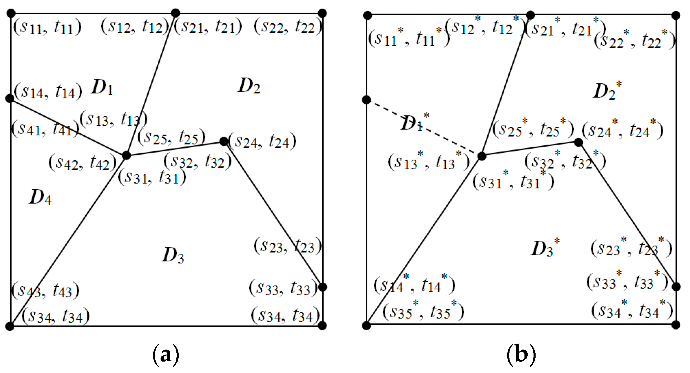
Figure 1 shows a partition of an image domain, D, by the proposed irregular tessellation, where D is partitioned into four polygons, such that D = {D₁, D₂, D₃, D₄}, and its node set is {P₁, P₂, P₃, P₄}, where P₁ = {(s₁₁, t₁₁), (s₁₂, t₁₂), (s₁₃, t₁₃), (s₁₄, t₁₄)}, P₂ = {(s₂₁, t₂₁), (s₂₂, t₂₂), (s₂₃, t₂₃), (s₂₄, t₂₄), (s₂₅, t₂₅)}, P₃ = {(s₃₁, t₃₁), (s₃₂, t₃₂), (s₃₃, t₃₃), (s₃₄, t₃₄)}, and P₄ = {(s₄₁, t₄₁), (s₄₂, t₄₂), (s₄₃, t₄₃)}. Thus, P = {(s₁₁, t₁₁), (s₁₂, t₁₂)/(s₁₂₁, t₂₁), (s₂₂, t₂₂), (s₁₄, t₁₄)/(s₄₁, t₄₁), (s₁₃, t₁₃)/(s₂₅, t₂₅)/(s₃₁, t₃₁)/(s₄₂, t₄₂), (s₂₄, t₂₄)/(s₃₂, t₃₂), (s₂₃, t₂₃)/(s₃₃, t₃₃), (s₃₅, t₃₅)/(s₄₃, t₄₃), (s₃₄, t₃₄)}. The symbol “/” indicates that both the nodes constructing different polygons are the same. P_im = {(s₁₁, t₁₁), (s₂₂, t₂₂), (s₃₅, t₃₅)/(s₄₃, t₄₃), (s₃₄, t₃₄)}. P_mm = P \ P_im. It is worth noting that, as the nodes on the image boundaries, (s₁₂, t₁₂)/(s₂₁, t₂₁), (s₁₄, t₁₄)/(s₄₁, t₄₁), (s₂₃, t₂₃)/(s₃₃, t₃₃) can only move along the boundary they are on.

2.2. Segmentation Model

Assume that a SAR image contains a known number, k, of homogeneous regions, and its domain is partitioned into an unknown number, m, of polygons by irregular tessellation, where m can be considered as a random variable and follows a prior distribution. Each polygon assigns a random variable, L_j, to indicate its membership to a homogeneous region. The label variables for all polygons form a label field, L = {L_j; j = 1, ..., m}. Let l = {l_j ∈{1, ..., k}; j = 1, ...., m} denote a realization of L, which corresponds to a segmentation result of the image.

According to the Bayesian theorem [21], a posterior probability as the segmentation model can be written as

$$p(m,L,P,\beta |Z)\propto p({\rm Z}|m,L,P,\beta )p(L|m)p(P|m)p(\beta )p(m)$$

(1)

where p(Z | m, L, P, β) is the likelihood model for the SAR image, characterized by gamma distribution [22],

$$p\left(Z|m,L,P,\beta \right)={\displaystyle \prod _{l=1}^k{\displaystyle \prod _{\left(x_i,y_i\right)\in {\Delta }_l}\frac{Z_i^{\alpha -1}}{\Gamma \left(\alpha \right){\beta }_l^{\alpha }}}}\exp \left(-\frac{Z_i}{{\beta }_l}\right)$$

(2)

where α and β = {β_l; l = 1, ..., k} are the shape and scale parameters of the gamma distribution, and Δ_l = {D_j: l_j = l, j = 1, ..., m} is the collection of polygons with the same label l. p(L| m) is the statistic model of the label field L, which can be defined based on the Markov random field (MRF) [23,24]

$$p\left(L|m\right)={\displaystyle \prod _{j=1}^{m}p\left(L_j|L_{j’},j’\in N_j\right)}={\displaystyle \prod _{j=1}^m\frac{\exp \left(c{\displaystyle \sum _{j’\in N_j}\delta \left(L_j,L_{j’}\right)}\right)}{{\displaystyle \sum _{l=1}^k\exp \left(c{\displaystyle \sum _{j’\in N_j}\delta \left(l,L_{j’}\right)}\right)}}}$$

(3)

where c > 0 is a constant that controls the neighborhood dependence between pairs of neighboring polygons [25] and δ is an indicator function,

$$\delta \left(L_j,L_{j’}\right)=\{\begin{array}{l}1,\mathrm{if}{L}_j=L_{j’}\\ 0,\mathrm{otherwise}\end{array}$$

(4)

p(P) is the joint prior distribution of the nodes in P, which is characterized by uniform distribution in the image domain D,

$$p(P|m)={\left(\frac{1}{D}\right)}^{n_p}={\left(D\right)}^{-n_p}$$

(5)

where n_p indicates the total number of images.

For a multi-look SAR intensity image, the shape parameters α of its gamma distribution can be viewed as the number of its looks [26]. p(β) is the joint distribution of {β_l; l = 1, ..., k}. Under the assumption that β_l, l = 1, ..., k, follow identical independent Gaussian distributions with the same distribution parameter μ_β and σ_β , p(β) can be expressed as

$$p\left(\beta \right)={\displaystyle \prod _{l=1}^k\frac{1}{\sqrt{2\pi }{\sigma }_{\beta }}}\exp \left[-\frac{{\left({\beta }_l-{\mu }_{\beta }\right)}^2}{2{\sigma }_{\beta }^2}\right]$$

(6)

p(m) is the prior distribution for the number of polygons, m, which is assumed to satisfy the Poisson distribution with mean λ [27],

$$p(m)=\frac{{\lambda }^m}{m!}\exp \left(-\lambda \right)$$

(7)

Using Equations (2)–(7), the segmentation model of Z defined in Equation (1) can be rewritten as

$$\begin{array}{l}p(m,L,P,\beta |Z)\propto p({\rm Z}|m,L,P,\beta )p(L|m)p(P|m)p(\beta )p(m)\\ ={\displaystyle \prod _{l=1}^k{\displaystyle \prod _{\left(x_i,y_i\right)\in {\Delta }_l}\frac{Z_i^{\alpha -1}}{\Gamma \left(\alpha \right){\beta }_l^{\alpha }}}}\exp \left(-\frac{Z_i}{{\beta }_l}\right)\times {\displaystyle \prod _{j=1}^m\frac{\exp \left(c{\displaystyle \sum _{j’\in N_j}\delta \left(L_j,L_{j’}\right)}\right)}{{\displaystyle \sum _{l=1}^k\exp \left(c{\displaystyle \sum _{j’\in N_j}\delta \left(l,L_{j’}\right)}\right)}}}\\ \times {\displaystyle \prod _{l=1}^k\frac{1}{\sqrt{2\pi }{\sigma }_{\beta }}}\exp \left[-\frac{{\left({\beta }_l-{\mu }_{\beta }\right)}^2}{2{\sigma }_{\beta }^2}\right]\times \frac{{\lambda }^m}{m!}\exp \left(-\lambda \right)\times {\left(D\right)}^{-n_p}\end{array}$$

(8)

2.3. Simulation

In order to obtain the optimal segmentation from Equation (8), a reversible-jump Markov chain Monte Carlo (RJMCMC) [28] algorithm was designed to simulate from the posterior probability and the maximum a posterior (MAP) [29] scheme was adopted. Using MAP, the optimal segmentation result could be expressed as

$$\left(\widehat{m},\widehat{L},\widehat{P},\widehat{\beta }\right)=\arg \max \left\{p\left(m,L,P,\beta |Z\right)\right\}$$

(9)

To obtain the optimal segmentation result, seven move operations were designed.

Move 1: Updating the gamma distribution parameter. Randomly select a scale parameter from β = {β_l; l = 1, ..., k}, for example β_l. The proposed β_l^* is drawn from a Gaussian distribution with the mean β_l and standard deviation ε_β (i.e., β_l^*~ N(β_l, ε_β)). The acceptance probability of changing β to β^* = {β₁, ..., β_l-1, β_l^*, β_l+1, ..., β_k} can be calculated as,

$${\alpha }_{\beta }=\min \left\{1,\frac{p\left(Z|m,L,P,{\beta }^{*}\right)p\left({\beta }^{*}|L\right)}{p\left(Z|m,L,P,\beta \right)p\left(\beta |L\right)}\right\}$$

(10)

Move 2: Updating the label. A polygon D_j with the label l_j is uniformly drawn with the probability 1/m from {D_j; j = 1, …, m}. To update its label, a proposed label l_j^* is uniformly drawn from {1, ..., k} and restricted to l_j^* ≠ l_j. The realization l = {l₁, ..., l_j, ..., l_m} of L after updating l_j to l_j^* becomes l ^* = {l₁, ..., l_j-1, l_j^*, l_j+1, ..., l_m}. The acceptance probability of changing l to l^* can be written as

$${\alpha }_L=\min \left\{1,\frac{p\left(Z|m,l^{*},P,\beta \right)p\left(l^{*}|m\right)}{p\left(Z|m,l,P,\beta \right)p\left(l|m\right)}\right\}$$

(11)

Move 3: Moving the node. A node is uniformly selected from mobile nodes P_mm (e.g., (s_jg, t_jg)) to move to a new proposed candidate point (s_jg^*, t_jg^*). If the node is located inside the image domain, the candidate point is selected randomly within a circle with the center at (s_jg, t_jg) and the radius r. If the node is on the boundary of the image, it can only move along the side of the boundary that it is on. If the node moves from (s_jg, t_jg) to (s_jg^*, t_jg^*), the polygon D_j is changed into D_j^*. Consequently, the set of the nodes for the polygon j, P_j = {(s_j1, t_j1), …, (s_jg, t_jg), …, (s_jnj, t_jnj)}, become P_j^*= {(s_j1, t_j1), …, (s_jg^*, t_jg^*), …, (s_jnj, t_jnj)}. The node sets for all polygons become P^* = P₁∪...∪P_j-1∪P_j^*∪P_j+1∪...∪P_m. Figure 2 shows two examples of the moving node operation, where Figure 2a,b shows the example of moving a node inside the image domain and Figure 2d the example of moving a node on the image boundary. After the moving node operation, the shapes of all the polygons related to the mobile node are changed.

The acceptance probability for the moving node can be written as

$${\alpha }_P=\min \left\{1,\frac{p\left(Z|m,L,P^{*},\beta \right)p\left(P^{*}|m\right)}{p\left(Z|m,L,P,\beta \right)p\left(P|m\right)}\right\}$$

(12)

Move 4: Merging polygons. A pair of neighbor polygons is selected, for example (D_j, D_j’) and j < j’. The two polygons D_j and D_j’ are merged into a candidate polygon D_j^*, and then the set of partitioned polygons {D₁, ..., D_j, ..., D_j’, ..., D_m} is changed into {D₁, ..., D_j^*, ..., D_m-1^*}. Accordingly, its node set P_j^* can be obtained as P_j^* = P_j ∪ P_j’ (specifically, delete the node located on the line). Then, the proposed l_j^* for the D_j^* is uniformly drawn from {1, ..., k} with the probability (1/k). The number of polygons after the merging polygons operation becomes m−1. The label field L = {L₁, ..., L_j, ..., L_j’, ..., L_m} becomes L^* = {L₁, ..., L_j^*, ..., L_m-1^*}. Figure 3 shows an example of merging polygons, where polygons D₁ and D₄ are selected to be merged as polygon D₁^*. The set of polygons D = {D₁, D₂, D₃, D₄} becomes D^* = {D₁^*, D₂^*, D₃^*}, where D₁^* = D₁ ∪ D₄.

The acceptance probability of merging polygons can be written as,

$${\alpha }_{MP}=\min \left\{1,\frac{p\left(Z|m-1,L^{*},P^{*},{\beta }^{*}\right)p\left(L^{*}|m-1\right)p\left(P^{*}|m-1\right)p\left(m-1\right)}{p\left(Z|m,L,P,\beta \right)p\left(L|m\right)p\left(P|m\right)p\left(m\right)}\right\}$$

(13)

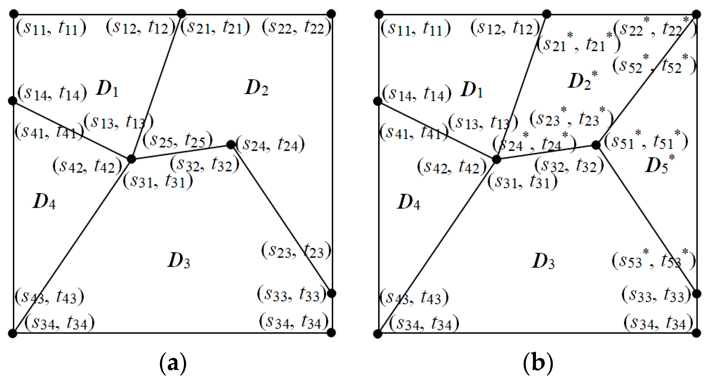
Move 5: Splitting polygons. A polygon with more than three nodes is selected randomly, for example D_j. A node (s_jg, t_jg) is selected from the node set P_j, randomly. Then another node is selected, for example (s_jg′, t_jg′), which is not adjacent to (s_jg, t_jg) from the node set P_j. The two selected nodes, (s_jg, t_jg) and (s_jg′, t_jg′), are then connected. As a result, D_j is split into two polygons, denoted as D_j^* and D_m+1^*. Correspondingly, P_j is divided into P_j^* ⊂ P_j and P_m+1^* ⊂ P_j. The P = {P₁, ..., P_j, ..., P_m} is changed to P^* = {P₁, ... ,P_j^*, ...,P_m^*, P_m+1}. Figure 4 shows an example of splitting a polygon, where the polygon D₂ is selected to be split into polygons D₂^* and D₃^*. The set of polygons D = {D₁, D₂, D₃, D₄} become D^* = {D₁, D₂^*, D₃, D₄, D₅^*}, where D₂ = D₂^* ∪ D₅^*.

The acceptance probability of splitting polygons can be written as

$${\alpha }_{SP}=\min \left\{1,\frac{p\left(Z|m+1,L^{*},P^{*},{\beta }^{*}\right)p\left(L^{*}|m+1\right)p\left(P^{*}|m+1\right)p\left(m+1\right)}{p\left(Z|m,L,P,\beta \right)p\left(L|m\right)p\left(P|m\right)p\left(m\right)}\right\}$$

(14)

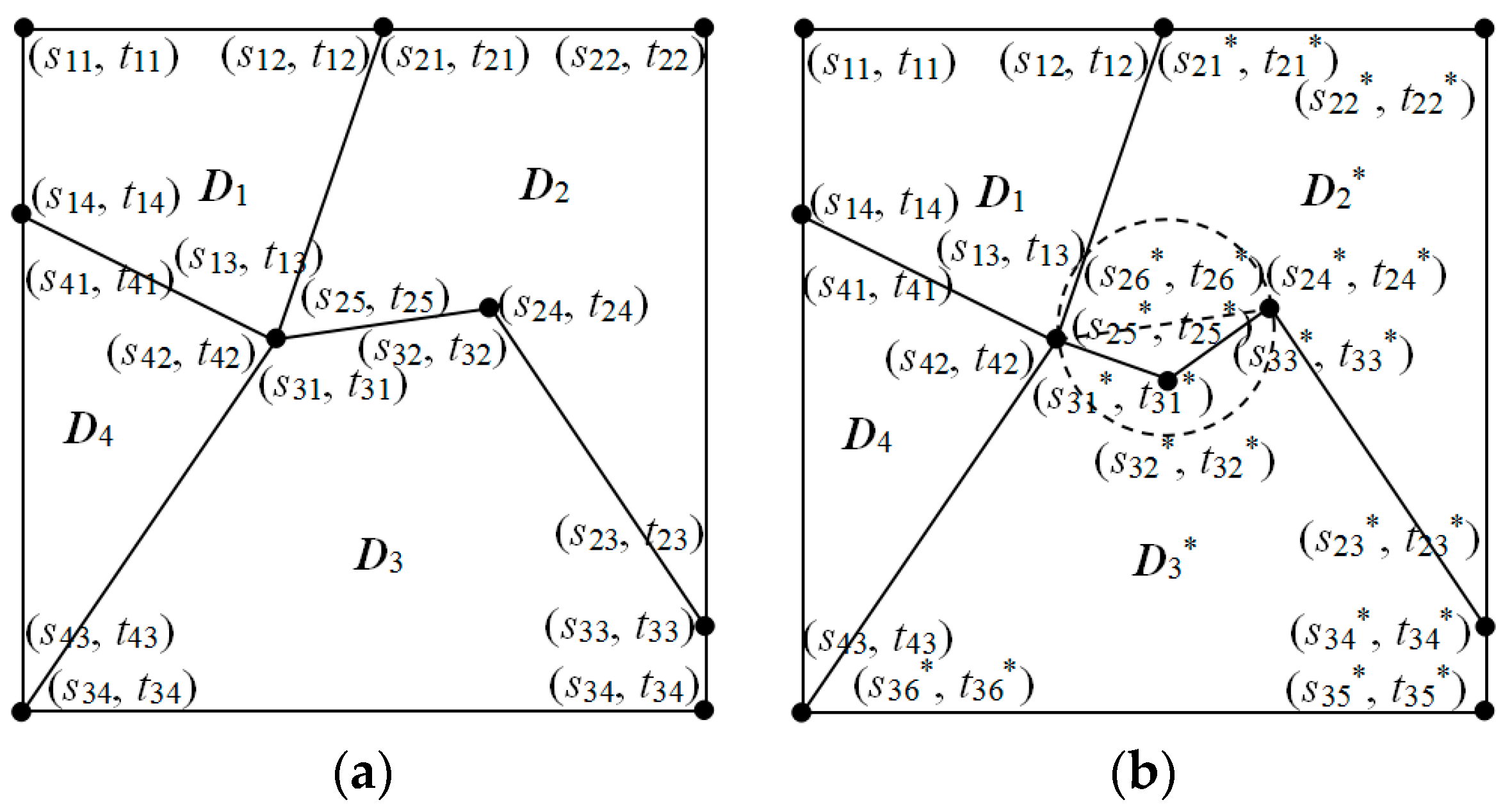
Move 6: Adding a node. For a randomly selected polygon, for example D_j, with one of its edges inside the image domain with the end points (s_jg, t_jg) and (s_jg+1, t_jg+1), a candidate node, denoted as (s_jnj+1, t_jnj+1), is uniformly drawn from the area from the intersection of the image domain and the circle with the center at the edge and the diameter equal to the length of the edge. Consequently, the set of nodes P_j = {(s_jg, t_jg) ∈ D; g = 1, …, n_j} is changed to P_j^*= {(s_jg, t_jg) ∈ D; g = 1, …, n_j+1}, and P_j’ = {(s_j’g, t_j’g) ∈ D; g = 1, …, n_j’} is changed to P_j’^*= {(s_j’g, t_j’g) ∈ D; g = 1, …, n_j’+1}. Additionally, the polygon D_j and its neighbor D_j’, which share the edge with D_j, are changed to D_j^* and D_j’^*, respectively. Figure 5 shows an example of adding a node, where the edge selected is made up of points (s₂₅, t₂₅) and (s₂₄, t₂₄) from D₂, and its neighbor polygon sharing the edge is D₃. After the operation, the number of nodes in polygon D₂ is transformed from five to six, while the number of nodes in polygon D₃ is also changed from five to six. Polygons D₂ and D₃ are changed into D₂^* and D₃^*, respectively.

The acceptance probability of adding a node can be written as

$${\alpha }_{AN}=\min \left\{1,\frac{p\left(Z|m,L,P^{*},\beta \right)p\left(P^{*}|m+1\right)}{p\left(Z|m,L,P,\beta \right)p\left(P|m\right)}\right\}$$

(15)

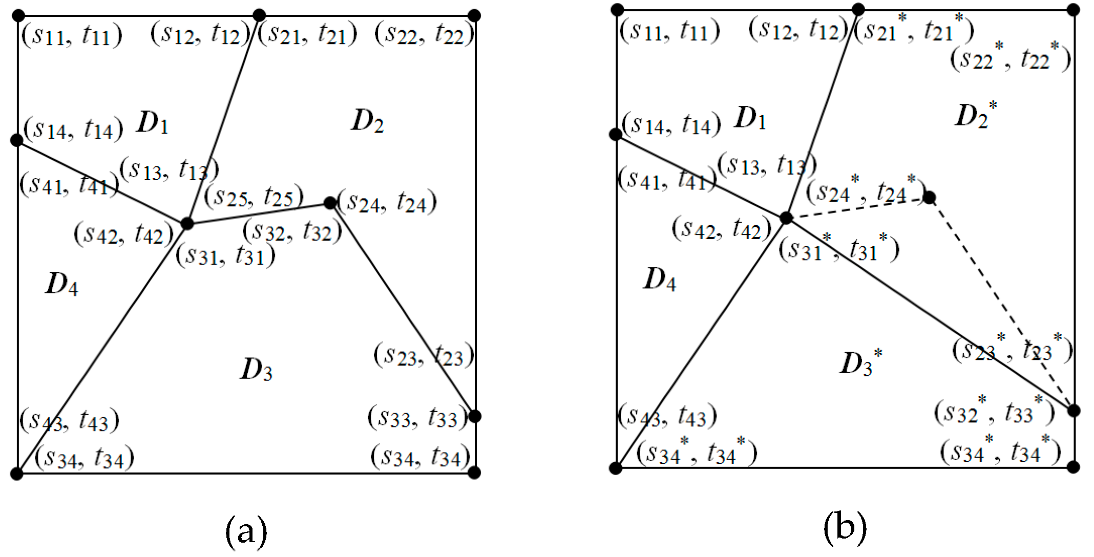
Move 7: Deleting a node. A concave polygon D_j is selected randomly from the current m polygons. Two adjacent edges are selected from D_j. The common node of the two edges is deleted. After deleting, the new edge can be generated by connecting the remaining nodes of the edges. Consequently, the set of nodes P_j = {(s_jg, t_jg) ∈ D; g = 1, …, n_j} is changed to P_j^*= {(s_jg, t_jg) ∈ D; g = 1, …, n_j-1}, and P_j’ = {(s_j’g, t_j’g) ∈ D; g = 1, …, n_j’} is changed to P_j’^*= {(s_j’g, t_j’g) ∈ D; g = 1, …, n_j’-1}. The polygons D_j and D_j’ are changed to D_j^* and D_j’^*, respectively. Figure 6 shows an example of deleting a node. The concave polygon is D₂, and its neighbor polygon is D_3. Two adjacent edges are selected from D₂, and then delete the common node, (s₂₄, t₂₄)/(s₃₂, t₃₂), of the edges. Thus, the remaining nodes, (s₁₃, t₁₃)/(s₂₅, t₂₅)/(s₃₁, t₃₁)/(s₄₂, t₄₂) and (s₂₃, t₂₃)/(s₃₃, t₃₃), are connected to generate a new edge. After the operation, the number of nodes of polygon D₂ is converted from five to four, and the number of nodes of polygon D₃ is also changed from five to four. Polygons D₂ and D₃ are changed into D₂^* and D₃^*, respectively.

The acceptance probability of deleting a node can be written as

$${\alpha }_{DN}=\min \left\{1,\frac{p\left(Z|m,L,P^{*},{\beta }^{}\right)p\left(P^{*}|m+1\right)}{p\left(Z|m,L,P,\beta \right)p\left(P|m\right)}\right\}$$

(16)

3. Experimental Results and Discussion

To verify the feasibility and effectiveness of the proposed algorithm, experiments were performed on both the simulated and intensity SAR images.

3.1. Experiment Setups

The proposed method was implemented by MATLAB programming and run on an Intel(R) Core (TM) i7-4790 CPU@ 3.6GHz 4G computer. The running time was about 30 min.

Table 1. Initial constant parameters.

Constants	m	c	μβ	σβ	εβ	Iteration
Value	16	1	32	8	1	10,000

lists the constants used in the proposed algorithm for the experiment. As the number of polygons changed by splitting and merging polygon operations, the value of the initial m had no significant impact on the results. In order to facilitate the following move operation, the initial tessellation partitioned the image domain D into 16 squares, such that the initial m = 16. The constant c was the coefficient used for characterizing the dependence of the neighboring polygons in the improved Potts model as defined in Equation (3), such that the conditional probability of the label for a polygon was a monotonic function. Based on a series of experiments, c ∈ [0.5, 1.5] was recommended [30]. In the experiment, the constant c was set to one. For multi-look SAR images, the shape parameter α of the gamma distribution was equal to the number of its looks. In the experiment, four-look SAR images were used for testing the proposed algorithm, such that α = 4. The initial scale parameters of gamma distribution were also drawn from their distributions, i.e., β_l ~ N(μ_β, σ_β), l = 1, ..., k. The values of the mean μ_β and standard deviation σ_β were set as 32 and 8, respectively. The constant ε_β was the proposed variance for β, which affects the convergence rate of the algorithm under the RJMCMC scheme. When ε_β is set to be too large, the parameter estimation is inaccurate, but if ε_β is set to be too small, the algorithm converges slowly. According to [31], the proper parameters can be obtained when ε_β is set to one. In the experiment, the number of iterations was set to 10,000. Generally, 10,000 iterations are sufficient to ensure convergence of the algorithm.

3.2. Simulated SAR Image Segmentation

To create a simulated image, a template of size 128 × 128 was constructed, as shown in Figure 7a. The number of homogeneous regions was three. For the simulated SAR image, each homogeneous region followed a gamma distribution, where the shape parameter was equal to four, and the scale parameter is listed in

Table 2. Parameter values of the gamma distributions for the simulated image.

Region.	I	II	III
Scale parameter (β)	5	25	45

. The simulated image is shown in Figure 7b. In order to verify the capability of fitting homogeneous regions with sharp angles in the proposed method, the simulated image was designed to have a sharp angle, as shown in Figure 7b highlighted by a blue rectangle. Figure 7c shows the zoomed image of the sharp angle area.

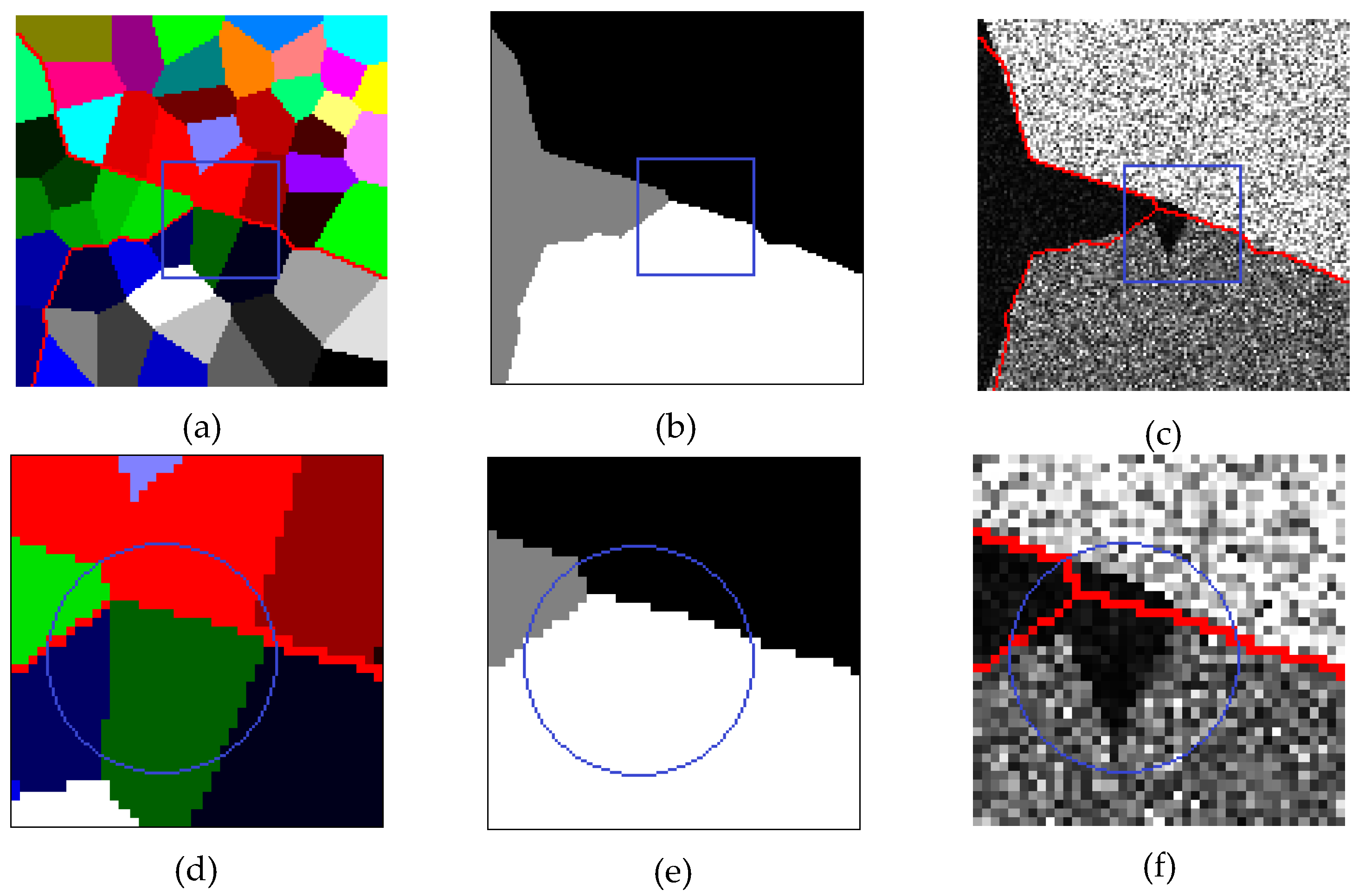
Figure 8 displays the segmentation results of the simulated image. Figure 8a shows the partition result from the irregular tessellation, and Figure 8b provides the optimal segmentation result. As shown in Figure 8a, each homogeneous region was fitted by one irregular polygon. To evaluate the proposed segmentation method qualitatively, the outlines of the segmented homogeneous regions (marked in red) were overlaid on the original image, as shown in Figure 8c. Figure 8d–f shows the zoomed-in images of the highlighted regions (in blue squares) from Figure 8a–c. As shown in Figure 8, the segmented regions from the proposed segmentation method perfectly fitted the homogeneous regions in the simulated image.

In order to verify the effectiveness of the proposed irregular partition method, the regular partition method [19] and Voronoi partition method [31] were used as comparison method. The results from the regular tessellation-based and Voronoi tessellation-based segmentation methods are illustrated in Figure 9 and Figure 10. The partition results of the regular and Voronoi tessellations are presented in Figure 9a and Figure 10a, the optimal segmentation results are provided in Figure 9b and Figure 10b, and the visual evaluation results are presented in Figure 9c and Figure 10c. Figure 9d–f and Figure 10d–f show the zoomed in images (in blue squares) from Figure 9a–c and Figure 10a–c, respectively. As shown in Figure 9, regular tessellation solved the problem of error segmentation caused by speckle noise in homogeneous regions to a certain extent, but boundary fitting results were coarse and uneven. From Figure 10, although the Voronoi polygons fitted most of the segments along the boundaries well, the results show that the method had difficulty matching the region with sharp angles (see Figure 10f).

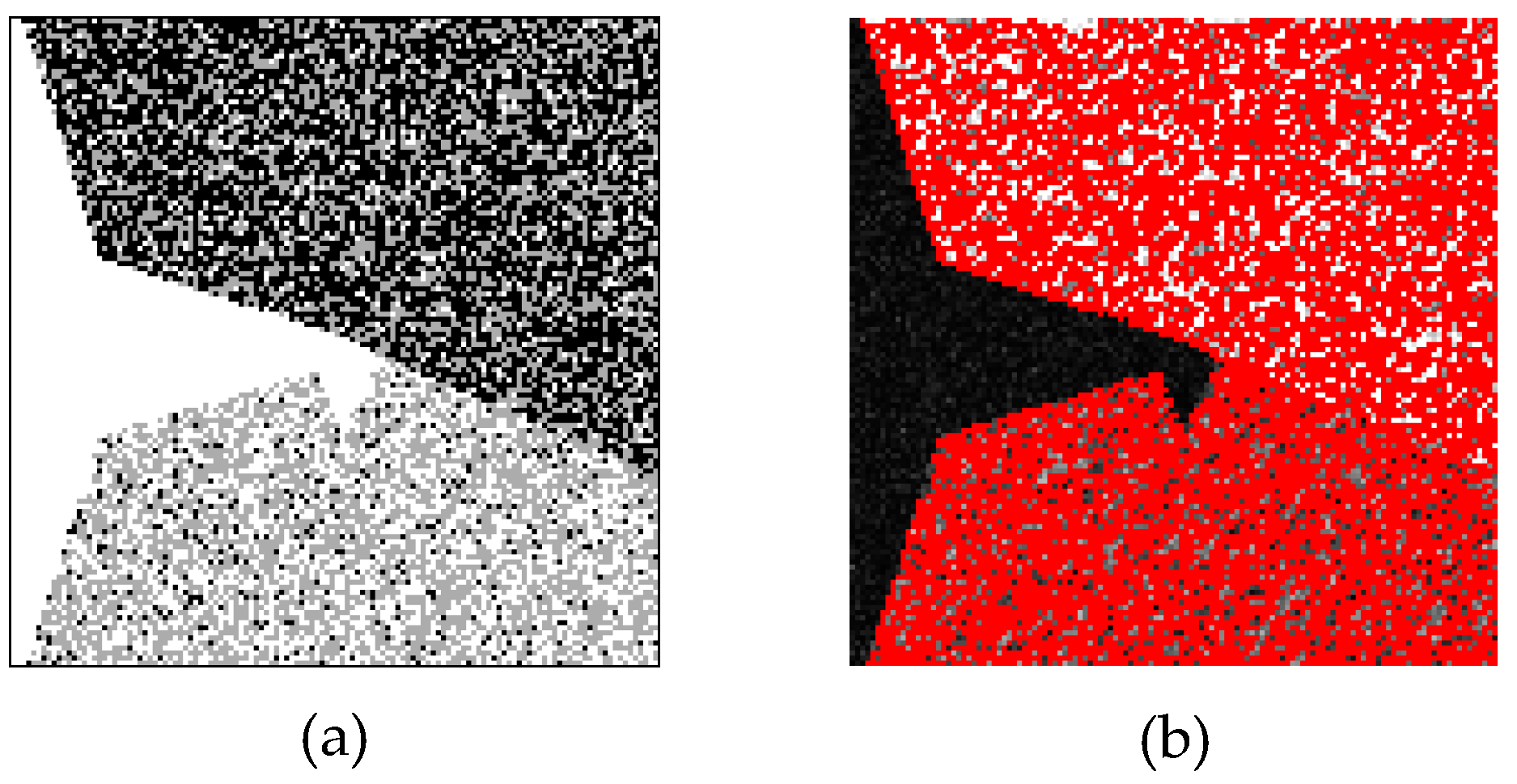
In order to verify the effectiveness of the proposed method for SAR image segmentation, the most classic multi-threshold method [32] was used as the contrast method to carry out experiments on the simulated SAR image, and the experimental results are shown in Figure 11. Figure 11a is the segmentation result. It can be seen that this method segmented region I better, but there were still many noises in regions II and III. In order to evaluate the experimental results qualitatively from the visual vision, the contour lines of the segmentation results were overlapped with the experimental image, as shown in the Figure 11b. It can be clearly seen that there was a lot of noise in regions II and III.

To evaluate quantitatively the effectiveness of all the segmentation methods, the confusion matrixes for their segmentation results (Figure 8b, Figure 9b, Figure 10b and Figure 11a) were calculated, taking the image from Figure 7a as a reference. Based on the matrixes, the producer’s accuracy, user’s accuracy, the overall accuracy, and the Kappa coefficient were calculated and listed in

Table 3. Quantitative evaluation of accuracy for the proposed method, the regular tessellation-based method, the Voronoi tessellation-based method, and the multi-threshold segmentation method.

		Region
	Method	I	II	III
User’s accuracy (%)	Proposed method	98.35	98.76	98.39
	Regular tessellation	83.33	97.45	99.58
	Voronoi tessellation	97.04	97.19	98.69
	Multi threshold	45.62	51.87	92.13
Producer’s accuracy (%)	Proposed method	94.91	98.36	99.85
	Regular tessellation	97.23	97.20	94.18
	Voronoi tessellation	90.81	98.65	99.71
	Multi threshold	100	50.43	57.12
Total accuracy (%)	Proposed method	98.57
	Regular tessellation	95.76
	Voronoi tessellation	97.89
	Multi threshold	61.59
Kappa	Proposed method	0.976
	Regular tessellation	0.932
	Voronoi tessellation	0.966
	Multi threshold	0.431

[33]. From Table 3, the overall precision of the proposed segmentation method was 98.57%, which demonstrates that the proposed method achieved excellent segmentation and was comparatively better than the regular, Voronoi tessellation-based segmentation methods and the multi-threshold segmentation method.

Figure 12 shows the changes of scale parameters throughout the 10,000 iterations for the different segmentation methods. Figure 12a–c shows the parameter variations of the proposed, the regular, and the Voronoi tessellation-based segmentation methods, respectively. From Figure 12a,c, the parameter for each homogeneous region converged to some steady value quickly (after about 1000 iterations). Figure 12b shows that the parameters were convergent but were not steady.

Table 4. Parameters obtained by the proposed method, regular tessellation, and Voronoi tessellation.

		Region
	Method	I	II	III
β	Proposed method	5.36	25.06	46.56
	Regular tessellation	25.77	29.66	46.25
	Voronoi tessellation	5.04	24.78	46.99
eβ (%)	Proposed method	7.20	0.24	3.47
	Regular tessellation	415.40	18.64	2.77
	Voronoi tessellation	0.80	0.88	4.42

provides the estimation values of the scale parameters and their percentage errors. It can be seen from Table 4 that the estimated parameters of the proposed and the Voronoi tessellation-based segmentation methods were more accurate than that of the regular tessellation-based segmentation method, particularly for region I. Figure 13 illustrates the histograms of the different homogeneous regions in the simulated image and the gamma distributions with real parameters. The histograms and the distribution function curves for the various homogeneous regions all matched accordingly.

3.3. Real SAR Intensity Images

Figure 14 presents four multi-look SAR intensity images with a size of 128 × 128 pixels, a spatial resolution of 30 m, and the number of looks equal to four. Figure 14a is a RADARSAT-1 image with HH polarization of a coastal scene, where the darker region indicates water (C1), and the brighter region represents the coast (C2). Figure 14b is a RADARSAT-II estuary image with HV polarization, where the darker regions indicate riverbanks (C1), and the middle portion marks ice (C2). Figure 14c is a RADARSAT-I image of sea ice with HH polarization. It contains three sea-ice structures, which from light to dark represent sea ice (C2), partially melted ice (C1), and water (C3), respectively. Figure 14d shows a RADARSAT-I standard-mode image with HH polarization, which shows four types of sea-ice structures, representative of different degrees of ice (light) and water (dark).

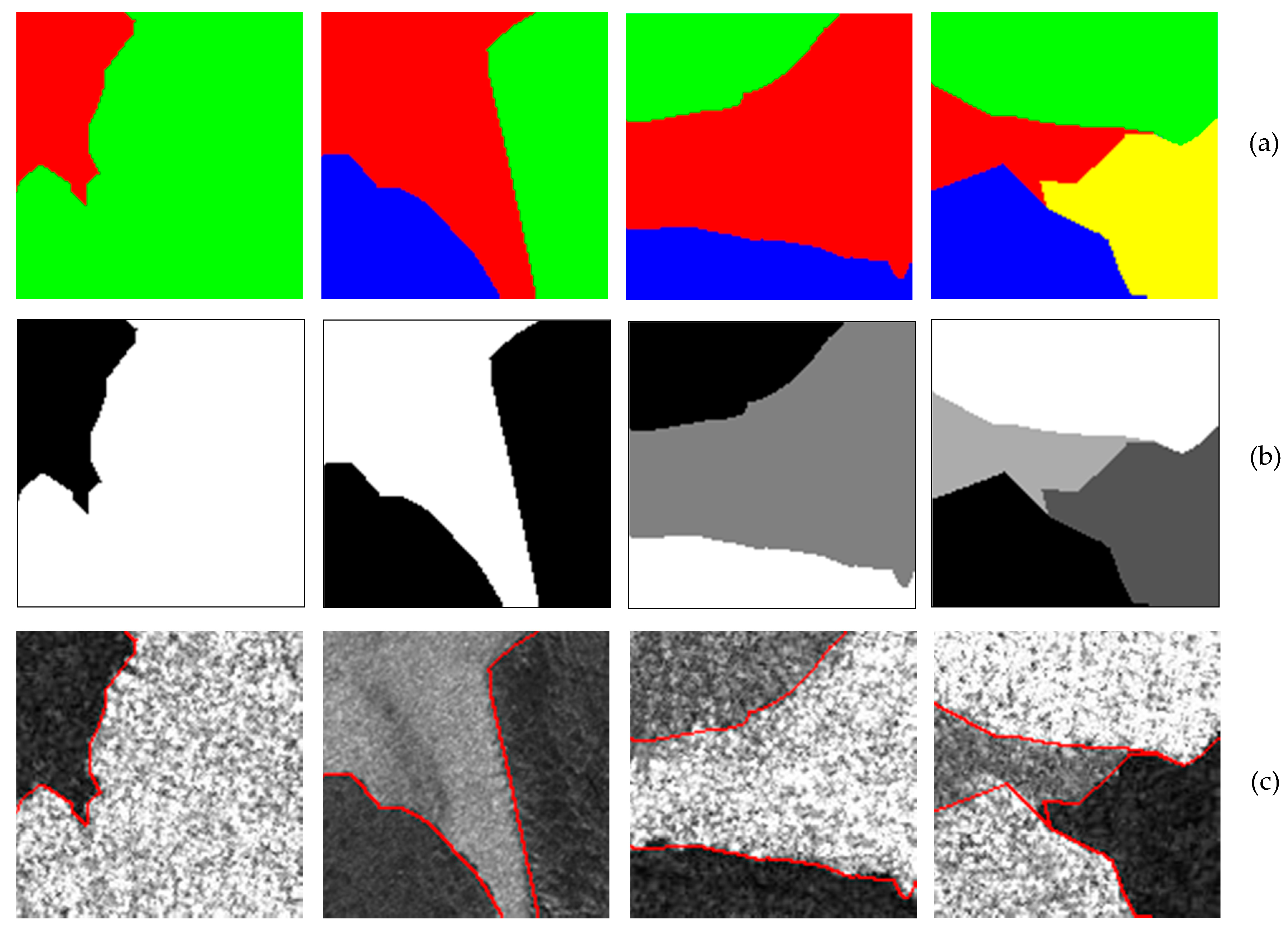
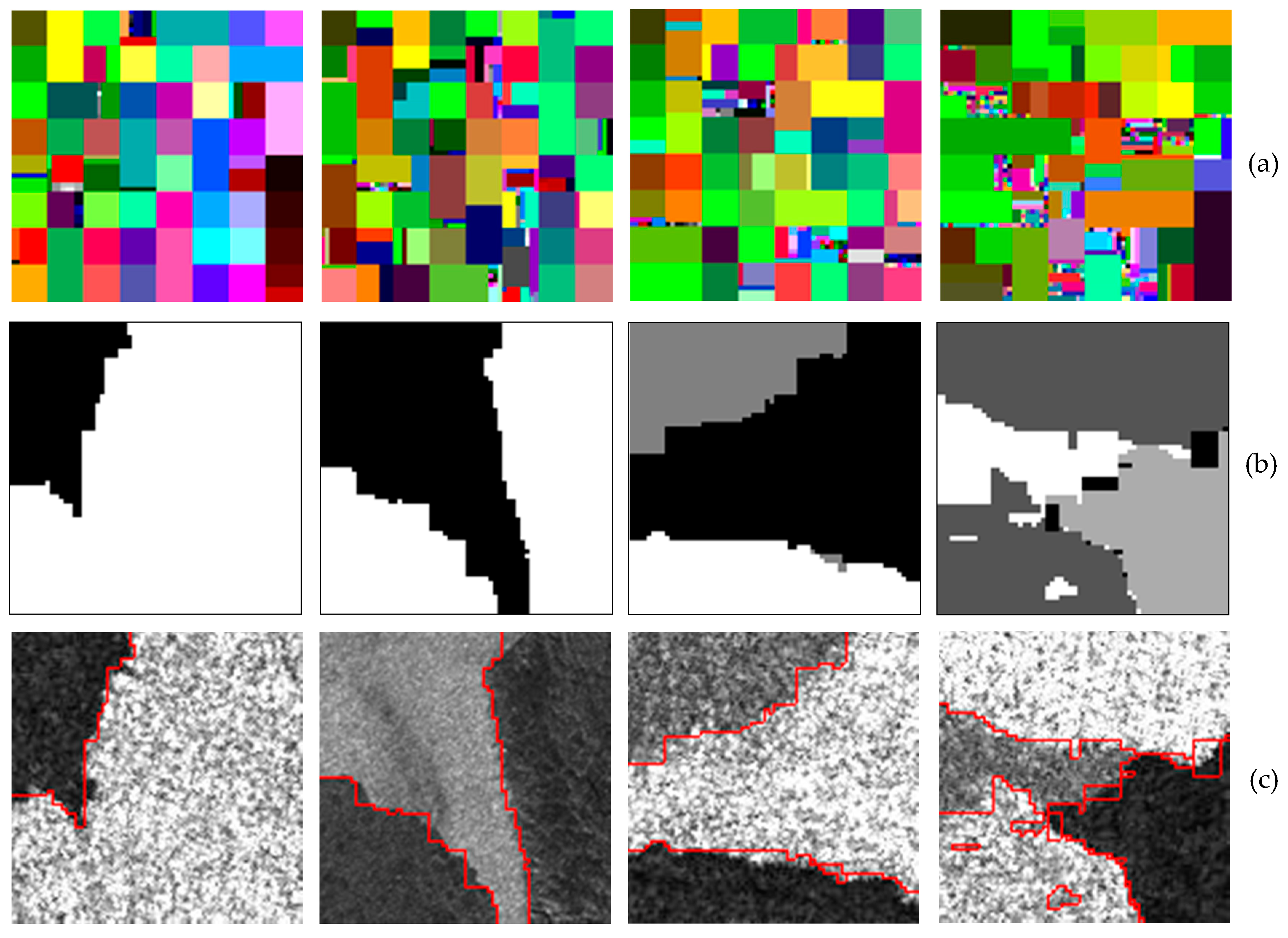
The proposed segmentation method was applied to the four SAR intensity images shown in Figure 14 using the same constants listed in Table 1. The segmentation results are shown in Figure 15. Figure 15a shows the result of dividing into irregular polygons. Figure 15b shows the segmentation results of the test images with varying numbers of homogeneous regions. In general, the number of irregular polygons should be the same as the number of homogeneous regions of the image. However, for non-adjacent homogeneous regions, the number of polygons was different from the number of homogeneous regions. As shown in the results of Figure 14b, the number of irregular polygons was three, while the number of homogeneous regions was two. This means that there were two polygons with the same label. In Figure 15c, the outlines of the segmented homogeneous regions were extracted and overlaid over the real images. From a visual examination, the proposed segmentation method was able to attain the optimal segmentation results.

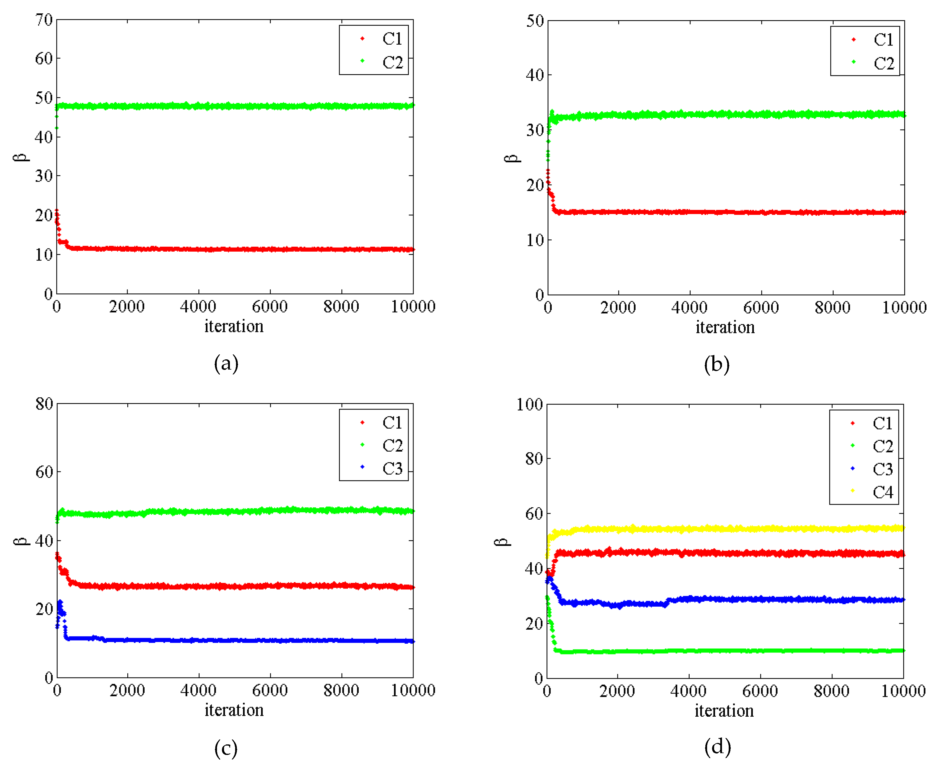
Figure 16 shows the variations of the scale parameters throughout the iteration process. The abscissa and ordinate represent the number of iterations and the scale parameter value, respectively. It can be seen from Figure 14 that the proposed segmentation method made the parameter value converge quickly and get stable parameter values.

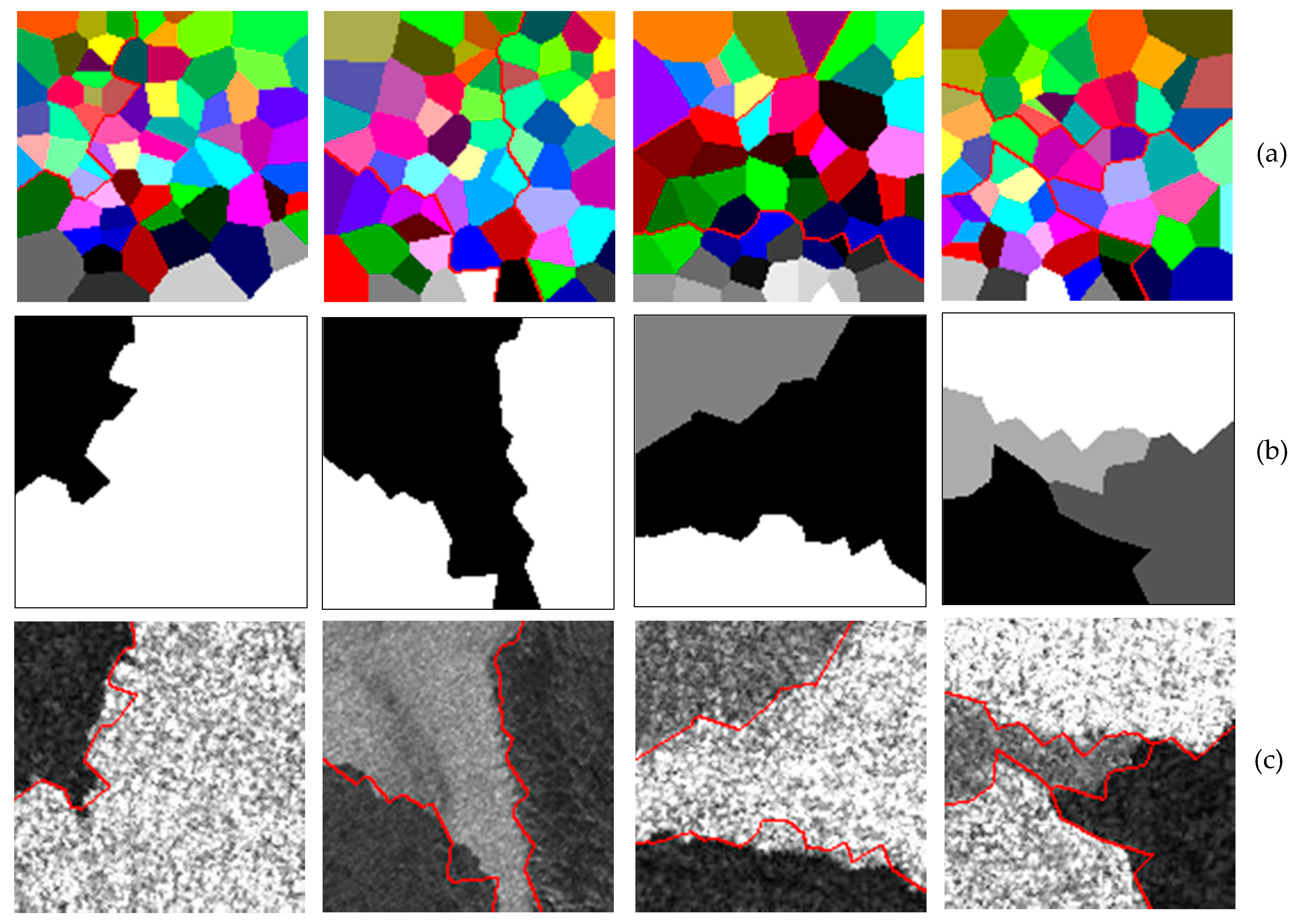
To compare the results of the proposed segmentation method, the real images shown in Figure 14 were tested using the regular and Voronoi tessellation-based segmentation methods; their segmentation results are shown in Figure 17 and Figure 18. There were some noises in the segmentation results of the regular tessellation method, as shown in Figure 17b. In Figure 18, the Voronoi tessellation-based segmentation method did not produce misclassified noise, but the boundary fitting was still not sufficiently accurate. Because the Voronoi polygons were convex, there were some constraints when using them to fit homogeneous regions.

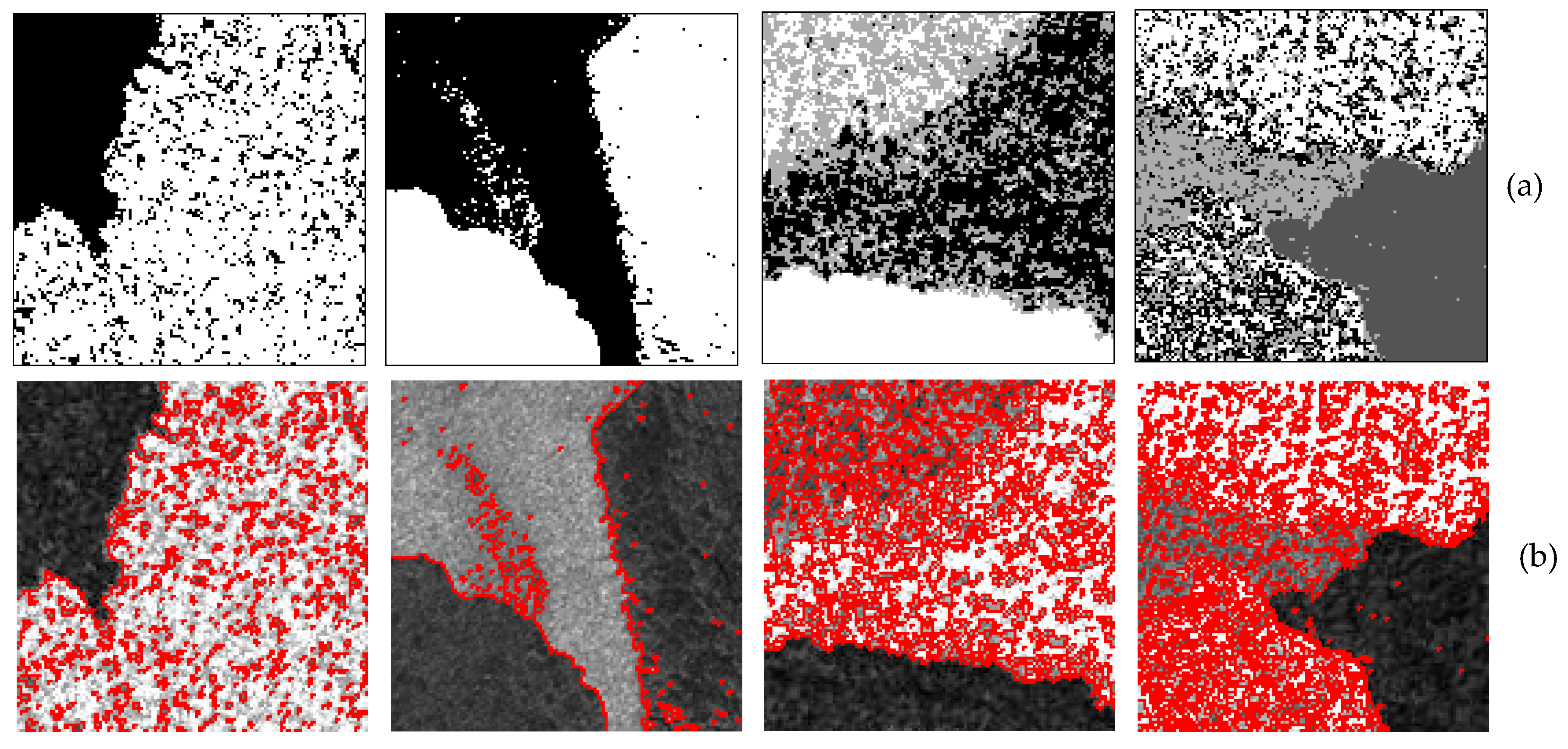
Figure 19 shows the experimental results of the multi-threshold segmentation method, where Figure 19a is the segmentation result and Figure 19b is the result of the overlap of the contour of the segmentation result and experimental image. It can be seen from the experimental results that this method had a good segmentation effect on the small difference in the pixel gray value (as shown in Figure 14b), but it was difficult to achieve a better segmentation result on the large difference in the pixel gray value.

4. Conclusions

This paper presents a new regional-based segmentation method for SAR intensity images. In this method, the image domain is partitioned into a collection of irregular polygons, which are constructed with a set of nodes and are used to fit homogeneous regions with arbitrary shapes. The commonly used regional-based segmentation method is based on either regular or Voronoi tessellations. The regular and Voronoi polygons can only fit in convex homogeneous regions but correspond poorly in areas with sharp corners. Compared with widely used segmentation methods, the proposed segmentation method provides greater flexibility, which can be used in both convex and concave homogeneous sections. As the nodes are used in segmenting sections, fewer polygons are needed to fit the homogeneous regions, resulting in more well-defined segments compared with other tessellation-based segmentation methods. Combining irregular tessellation and Bayesian inference to segment SAR images, the experiment results show that the proposed segmentation method can provide better segmentation results and, at the same time, the model parameters can be estimated more accurately. The proposed irregular tessellation method provides a new idea for region-based image segmentation and a better solution for region segmentation with different geometric shapes. However, it has no effect on the image category (sea ice, city, and forest). This paper only takes low-resolution SAR sea-ice images as examples for simple verification. In future work, high-resolution urban and forest images can be considered for segmentation experiments to verify the universality of the proposed method.

References

1. Oliver, C.; Quegan, S. Understanding Synthetic Aperture Radar Images; Artech House: Boston, UK, 1998; pp. 277–296. [Google Scholar]
2. Dong, G.G.; Kuang, G.Y.; Wang, N.; Zhao, L.J. SAR target recognition via joint sparse representation of monogenic signal. IEEE J.-STARS 2017, 8, 3316–3328. [Google Scholar] [CrossRef]
3. Zhang, S.; He, F.; Zhang, Y.; Wang, J.M.; Mei, X.; Feng, T.T. Geometric active contour based approach for segmentation of high-resolution spaceborne SAR images. J. Syst. Eng. Election. 2015, 26, 69–76. [Google Scholar] [CrossRef]
4. Li, M.X.; Cheng, J.L. SAR image segmentation based on watershed and spectral clustering. J. Infrared Millim. W 2008, 27, 452–456. [Google Scholar]
5. Li, W.; Benie, G.B.; He, D.C.; Wang, S.R.; Ziou, D.; Hugh, Q.; Gwyn, J. Watershed-based hierarchical SAR image segmentation. Int. J. Remote Sens. 1999, 20, 3377–3390. [Google Scholar] [CrossRef]
6. Ayed, I.B.; Mitiche, A.; Belhadj, Z. Multiregion level-set partitioning of synthetic aperture radar images. IEEE Trans. Pattern Anal. Mach. Intell. 2005, 27, 793–800. [Google Scholar] [CrossRef]
7. Roger, F.; Armand, L.; Philippe, M.; Eliane, C.C. An optimal multiedge detector for SAR image segmentation. IEEE Trans. Geosci. Remote Sens. 1998, 36, 793–802. [Google Scholar]
8. Germain, O.; Refregier, P. Edge location in SAR images: Performance of the likelihood ratio filter and accuracy improvement with an active contour approach. IEEE Trans. Image Process. 2001, 10, 72–78. [Google Scholar] [CrossRef]
9. Smith, D.M. Speckle reduction and segmentation of Synthetic Aperture Radar images. Int. J. Remote Sens. 1996, 17, 2043–2057. [Google Scholar] [CrossRef]
10. Quan, J.J.; Wen, X.B.; Xu, X.Q. Multiscale probabilistic neural network method for SAR image segmentation. Appl. Math. Comput. 2008, 205, 578–583. [Google Scholar] [CrossRef]
11. Galland, F.; Bertaux, N.; Refregier, P. Minimum description length synthetic aperture radar image segmentation. IEEE Trans. Image Process 2003, 12, 995–1006. [Google Scholar] [CrossRef] [Green Version]
12. Cremers, D.; Rousson, M.; Deriche, R. A review of statistical approaches to level set segmentation: Integrating color, texture, motion and shape. Int. J. Comput. Vis. 2007, 72, 195–215. [Google Scholar] [CrossRef] [Green Version]
13. Lei, X.; Li, Y.; Zhao, N. Fast segmentation approach for SAR image based on simple Markov random field. J. Syst. Eng. Election. 2010, 21, 31–36. [Google Scholar] [CrossRef]
14. Zhao, Q.H.; Li, Y.; He, X.J.; Song, W.D. Multi-look SAR image segmentation based on voronoi tessellation technique and EM/MPM algorithm. J. Remote Sens. 2013, 17, 841–854. [Google Scholar]
15. Comer, M.L.; Delp, E.J. The EM/MPM algorithm for segmentation of textured images: Analysis and further experimental results. IEEE Trans. Image Process. 2000, 9, 1731–1744. [Google Scholar] [CrossRef]
16. Hou, Y.M. A novel SAR image segmentation method based on markov random field. J. Electron. Inf. Technol. 2007, 29, 1069–1072. [Google Scholar]
17. Yang, Y.; Sun, H.; He, C. Supervised SAR image MPM segmentation based on region-based hierarchical model. IEEE Geosci. Remote Sens. 2006, 3, 517–521. [Google Scholar] [CrossRef]
18. Dryden, I.L.; Farnoosh, R.; Taylor, C.C. Image segmentation using Voronoi polygons and MCMC, with application to muscle fibre images. J. Appl. Stat. 2006, 33, 609–622. [Google Scholar] [CrossRef]
19. Wang, Y.; Li, Y.; Zhao, Q.H. Segmentation of high-resolution SAR image with unknown number of classes based on regular tessellation and RJMCMC algorithm. Int. J. Remote Sens. 2015, 36, 1290–1306. [Google Scholar] [CrossRef]
20. Zhao, Q.H.; Li, Y.; Wang, Y. SAR image segmentation with unknown number of classes combined Voronoi tessellation and RJMCMC algorithm. ISPRS Ann. Photogramm. Remote Sens. Spat. Inf. Sci. 2016, 3, 119–124. [Google Scholar] [CrossRef]
21. Julian, B. Towards Bayesian image analysis. J. Appl. Stat. 1989, 16, 395–406. [Google Scholar]
22. Dong, Y.; Forster, B.C.; Milne, A.K. Comparison of radar image segmentation by Gaussian and Gamma-Markov random field models. Int. J. Remote Sens. 2003, 24, 711–722. [Google Scholar] [CrossRef]
23. Besag, J. On the statistical analysis of dirty picture (with discussion). J. R. Stat. Soc. B 1986, 48, 259–302. [Google Scholar]
24. Strauss, D.J. Clustering on coloured lattices. J. Appl. Prob. 1977, 14, 135–143. [Google Scholar] [CrossRef]
25. Dryden, I.; Scarr, M.R.; Taylor, C.C. Bayesian texture segmentation of weed and crop image using reversible jump Markov chain Monte Carlo methods. J. R. Stat. Soc. Ser. C Appl. Stat. 2003, 52, 31–50. [Google Scholar] [CrossRef]
26. Richards, J.A. Remote Sensing with Imaging Radar; Springer: Berlin/Heidelberg, Germany, 2009; pp. 1–373. [Google Scholar]
27. Zhao, Q.H.; Zhang, H.Y.; Li, Y. Detecting dark spots from SAR intensity images by a point process with irregular geometry marks. Int. J. Remote Sens. 2018. [Google Scholar] [CrossRef]
28. Green, J. Reversible jump Markov chain Monte Carlo computation and Bayesian model determination. Biometrika 1995, 82, 711–732. [Google Scholar] [CrossRef]
29. Bernardo, J.M.; Smith, A.F.M. Bayesian Theory; Wiley: New York, NY, USA, 1994; pp. 1–606. [Google Scholar]
30. Li, Y.; Li, J. Segmentation of SAR intensity imagery with a Voronoi tessellation, bayesian inference, and reversible jump MCMC algorithm. IEEE Trans. Geosci. Remote Sens. 2010, 48, 1872–1881. [Google Scholar] [CrossRef]
31. Zhao, Q.H.; Li, Y.; Liu, Z.G. SAR image segmentation using Voronoi tessellation and Bayesian inference applied to dark spot feature extraction. Sensors 2013, 13, 14484–14499. [Google Scholar] [CrossRef] [Green Version]
32. Otsu, N. A Threshold Selection Method from Gray-Level Histograms. IEEE Trans. Syst. Man Cybern. 1979, 9, 62–66. [Google Scholar] [CrossRef] [Green Version]
33. Congaltonr, G.; Green, K. Assessing the Accuracy of Remotely Sensed Data: Principles and Practices, 2nd ed.; CRC Press: Boca, Ration, FL, USA, 2008; pp. 169–190. [Google Scholar]
Figure 1. Irregular tessellation with four polygons, where the symbol • indicates node.
Remotesensing 12 00753 g001
Figure 2. Example of moving one mobile node. (a) initial division; (b) relocated node within the image; (c) initial division; (d) relocated node along the boundary.
Remotesensing 12 00753 g002
Figure 3. Example of merging polygons. (a) initial division; (b) merged polygon.
Remotesensing 12 00753 g003
Figure 4. Example of splitting a polygon. (a) initial division; (b) split polygon.
Remotesensing 12 00753 g004
Figure 5. Example of adding a node. (a) initial division; (b) after one node is added.
Remotesensing 12 00753 g005
Figure 6. Example of deleting a node. (a) Initial division; (b) One node deleted.
Remotesensing 12 00753 g006
Figure 7. Irregular tessellation with four polygons. (a) template image; (b) simulated image; (c) Enlarge image.
Remotesensing 12 00753 g007
Figure 8. Experimental result of proposed method. (a) irregular tessellation result; (b) segmentation result; (c) visual evaluation; (d) magnified irregular tessellation result; (e) magnified segmentation result; (f) magnified visual evaluation image.
Remotesensing 12 00753 g008
Figure 9. Experimental results of the regular tessellation-based method. (a) regular tessellation result; (b) segmentation result; (c) visual evaluation; (d) magnified regular tessellation result; (e) magnified segmentation result; (f) magnified visual evaluation image.
Remotesensing 12 00753 g009
Figure 10. Experimental results of the Voronoi-tessellation-based method. (a)Voronoi tessellation result; (b) segmentation result; (c) visual evaluation; (d) magnified Voronoi tessellation result; (e) magnified segmentation result; (f) magnified visual evaluation.
Remotesensing 12 00753 g010
Figure 11. Experimental results of multi-threshold segmentation. (a) segmentation result; (b) visual evaluation.
Remotesensing 12 00753 g011
Figure 12. Changes in scale parameters through iteration. (a) parameter variations of the proposed method; (b) parameter variations of regular tessellation; (c) parameter variations of Voronoi tessellation.
Remotesensing 12 00753 g012
Figure 13. Histograms and curves of gamma distributions with real and estimated model parameters. (a) Region I; (b) Region II; (c) Region III.
Remotesensing 12 00753 g013
Figure 14. Real SAR intensity images.
Remotesensing 12 00753 g014
Figure 15. Segmentation results and visual evaluation. (a) irregular tessellation results; (b) segmentation results; (c) visual evaluation.
Remotesensing 12 00753 g015
Figure 16. Curves of parameter variations with number of iterations. (ad) represent the scale parameter changes of each homogeneous region in the four remote sensing images in Figure 14.
Remotesensing 12 00753 g016
Figure 17. Segmentation results and visual evaluations of the regular tessellation method. (a) regular tessellation results; (b) segmentation results; (c) visual evaluation.
Remotesensing 12 00753 g017
Figure 18. Segmentation results and visual evaluations of the Voronoi tessellation method. (a) Voronoi tessellation results; (b) segmentation results; (c) visual evaluation.
Remotesensing 12 00753 g018
Figure 19. Segmentation results and visual evaluations of the multi-threshold segmentation. (a) segmentation results; (b) visual evaluation.
Remotesensing 12 00753 g019