Woody Cover Fractions in African Savannas From Landsat and High-Resolution Imagery

Abstract

The challenge of mapping savanna vegetation has limited our understanding of the factors that shape these ecosystems at large scales. We tested seven methods for mapping savanna woody cover (trees and shrubs; WC) across 12 protected areas (PAs) in eastern Africa using Landsat 8 imagery. Because we wanted a method viable for mapping across the often-limited Landsat historical archive, we limited ourselves to three images: one each from the wet, dry, and transition (halfway between wet and dry) seasons. Models were trained and tested using 1,330 WC reference points and the variance explained by cross validation (VEcv) accuracy metric. Of the methods we tested, RF significantly (p < 0.001) outperformed the others with the best models in nine PAs scoring over 75% (range of 34.5%–91.1%). RF models trained using data from all the PAs and tested in the individual PAs significantly (p < 0.001) outperformed their single-PA-derived counterparts (67.7 ± 23.3% versus 30.5 ± 27.4%). We also found that while the transition image appears to be critical to mapping WC and the wet season image should be avoided, no single season or seasonal combination significantly outperformed all the others, allowing some flexibility in image selection. Our findings show that with proper sampling of landscape heterogeneity, even with limited imagery, accurate maps of savanna WC are possible and could catalyze discoveries in this crucial biome.

1. Introduction

Savannas cover a fifth of earth’s land surface [1] and are home to over 500 million people (estimate derived by intersecting The Nature Conservancy’s savanna and shrubland ecoregions [2] with population estimates for 2015 [3]). Defined as mixed tree-grass communities [4], savannas support pastoralist cultures [5], the world’s largest, functionally complete set of terrestrial megafauna [6] and thriving tourist economies [7,8]. Savannas also play a disproportionate role in the interannual variability of the global carbon cycle [9,10]. In all of these, the woody cover (WC; i.e., trees and shrubs) of savannas plays an important role: pastoralism, tourism, and grazing wildlife all rely on sparse WC and are threatened by woody encroachment [5,11,12], while savanna carbon dynamics are disproportionately affected by woody vegetation [4,13]. Yet, our understanding of the factors controlling savanna WC, in comparison to other biomes (i.e., grasslands and forests), is relatively limited.

Unlike the climate-determined WC of forests and grasslands, savanna WC exists in a climate-indeterminate state [14]. In savannas, disturbances work individually or synergistically to maintain low WC in areas that might otherwise transition to forest or grassland [15,16], a characteristic termed “multiple stable states” [17,18]. Chief among the disturbances are fire [19,20,21], drought [22,23,24] and herbivory [25,26,27,28]. However, despite efforts to understand how disturbances interact with each other and climate across broad spatial scales [16,29], our ability to predict savanna WC to any significant degree is still limited [30].

Part of the challenge of understanding savannas has likely come from the data used in prior studies. Several influential studies of savannas and/or multiple stable states [31,32,33,34,35,36] centered on analyses of Vegetation Continuous Fields (VCF) global tree cover data [37]—data now known to have significant inaccuracies in savannas [38,39,40]. Consequently, the producers of the dataset cautioned against the use of VCF in areas with less than 20–30% tree cover [38], effectively ruling out savannas given their characteristic ~20% mean VCF tree cover [32]. Additionally, VCF, which was primarily developed to monitor forests, not savannas, defines trees as woody vegetation >5 m tall [37]. While a fair threshold for forests, the majority of savanna woody vegetation likely falls below it [41], thus under-representing the woody component of these systems. More importantly, disturbances predominately act upon woody vegetation recruits (< ~5–6 m) [19,25,41,42,43,44], meaning VCF is unlikely to detect the direct impacts of disturbances, i.e., the major determinants of WC. Combined, these factors make the use of VCF in any savanna problematic, potentially undermining our ability to understand these ecosystems.

In lieu of VCF, researchers often make maps of their own. However, making large-scale maps of savanna WC is a challenge because, unlike in forests, savanna imagery contains a high proportion of pixels with a combination of woody vegetation, herbaceous vegetation, and bare soil—referred to as mixed pixels [45,46]. Unmixing pixels requires knowledge of the spectral characteristics of all the materials within the pixel. Meeting that requirement across large areas has been a long-standing challenge [47] because vegetation and soil spectral properties change across space and time, particularly in savannas [37,38,48,49].

To limit the spectral variability of cover types, researchers often produce small-scale, site-specific maps using a range of approaches, including simple linear regressions [50], regression trees [51], cluster analysis [52], and spectral unmixing [53]. Meanwhile, some of those who have attempted to produce maps across larger areas or across several sites abandoned such approaches, instead manually classifying a high number small areas (~0.5 hectare) using very high-resolution (VHR; < 1 m) imagery [54,55] or, in an effort to lower VCF error, resampling the data to coarser resolutions, thereby abandoning fine scale analysis [34]. Still others use commercially produced national landcover maps [56]. The different data sources and methodologies mean maps are rarely easily comparable across studies. That, combined with an overall shortage of these maps, limits large-scale studies of savanna dynamics, while also limiting our ability to compare the approaches used to generate them. Further, studies rarely map WC across time, despite the demonstrated insights from temporal data [36,57,58].

Here, we develop an accurate, replicable method for mapping total WC across 12 protected areas in eastern Africa, from Uganda to South Africa, using Landsat 8 imagery. While we recognize separate maps of shrub cover and tree cover would be ideal when studying savannas and could be possible using ancillary data (e.g., LiDAR-derived digital surface models), we sought a method that could be applied through time, back to the launch of Landsat 4 (1982)—a span that extends beyond most ancillary data. Further, we chose to not use ancillary data that could be assumed to be constant across the temporal record (e.g., topography) to avoid circularity in future studies of landscape-scale controls on savanna distributions and WC. Last, given the marked decline in Landsat image availability going back to the 1990s and 1980s, especially in rural Africa [59], we limited ourselves to three images per site: one each from the wet and dry seasons, along with the transition between them. The result was the development of 30-m resolution maps of WC fractions across all the sites; site-specific rankings of seasonal imagery; a novel approach for reference data generation; and a clear designation of the best mapping approach.

2. Materials and Methods

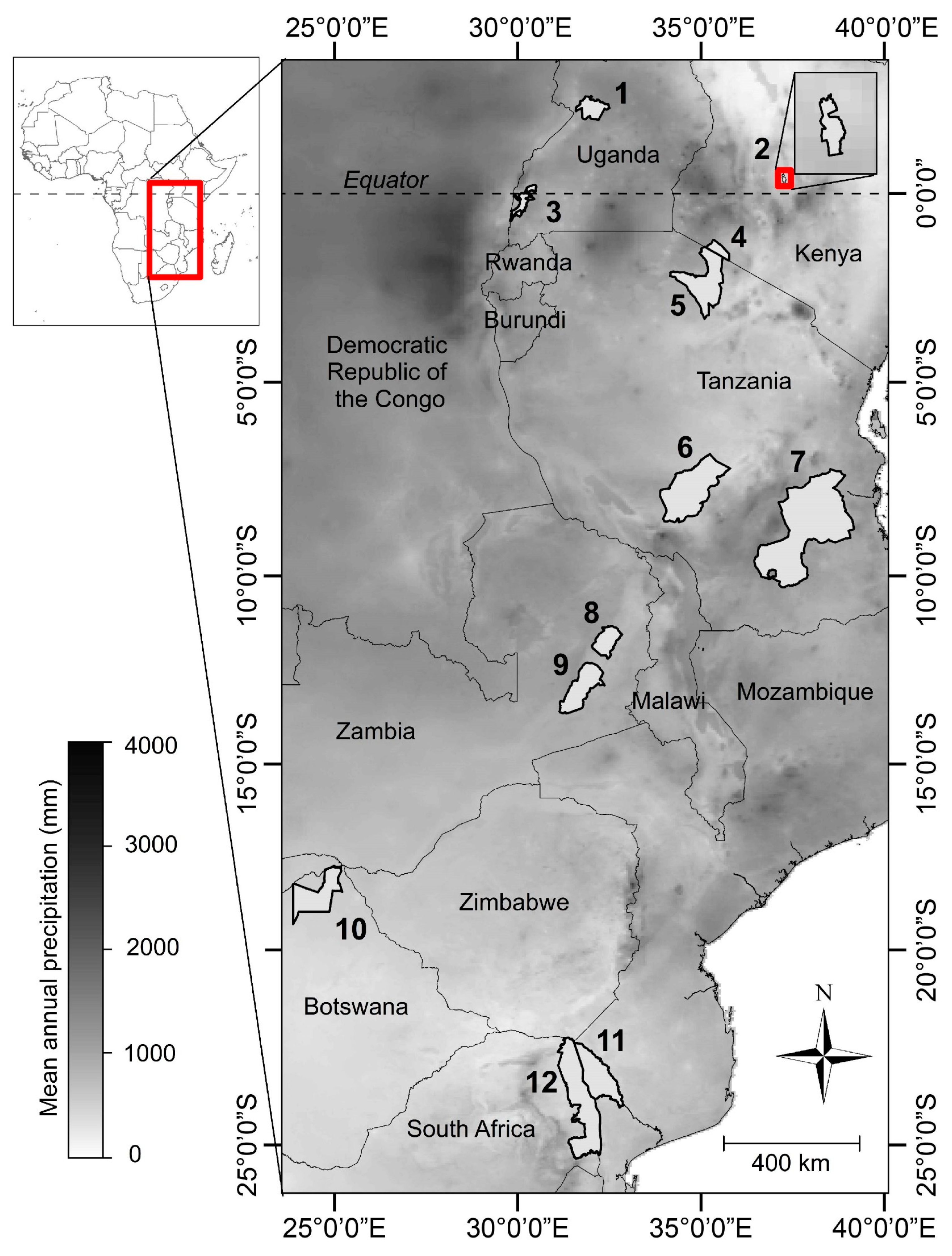
2.1. Study Sites

We mapped WC in 12 sites across eastern and southern Africa (Figure 1;

Table 1. Protected area names, abbreviations and attributes, listed from north to south. PA numbering corresponds to Figure 1.

PA #	Name and Country	Abbr.	Latitude (Degrees)	Elev. (m)	MAP (mm)	Area (km2)
1	Murchison Falls National Park, Uganda	MUR	2.27	846	1262	3877
2	Mpala Research Center, Kenya	MPA	0.40	1694	601	194
3	Queen Elizabeth National Park, Uganda	QUE	−0.25	977	998	7395
4	Masai Mara National Reserve, Kenya	MAR	−1.50	1624	950	1510
5	Serengeti National Park, Tanzania	SER	−2.27	1546	850	14763
6	Ruaha National Park, Tanzania	RUA	−7.80	1168	700	20226
7	Selous Game Reserve, Tanzania	SEL	−8.86	396	1121	44800
8	North Luangwa National Park, Zambia	NLU	−11.88	752	904	4636
9	South Luangwa National Park, Zambia	SLU	−13.09	623	917	9050
10	Chobe National Park, Botswana	CHO	−18.56	968	532	11000
11	Limpopo National Park, Mozambique	LIM	−23.32	246	534	10000
12	Kruger National Park, South Africa	KRU	−23.93	342	511	19175

). All of our sites are protected areas (International Union for Conservation of Nature protected status II–IV). We selected protected areas (PAs) because, as part of a larger project studying the drivers of savanna processes, we sought to avoid modern anthropogenic impacts to the extent possible, though we recognize that humans have long played a role in savannas [60,61,62]. The PAs cover a broad range of mean annual precipitation (MAP) (~500–1250 mm) and size (~200–44,800 km²). Initial inspection using satellite imagery suggested the PAs also cover a broad range of WC, with wetter PAs appearing significantly woodier than drier PAs.

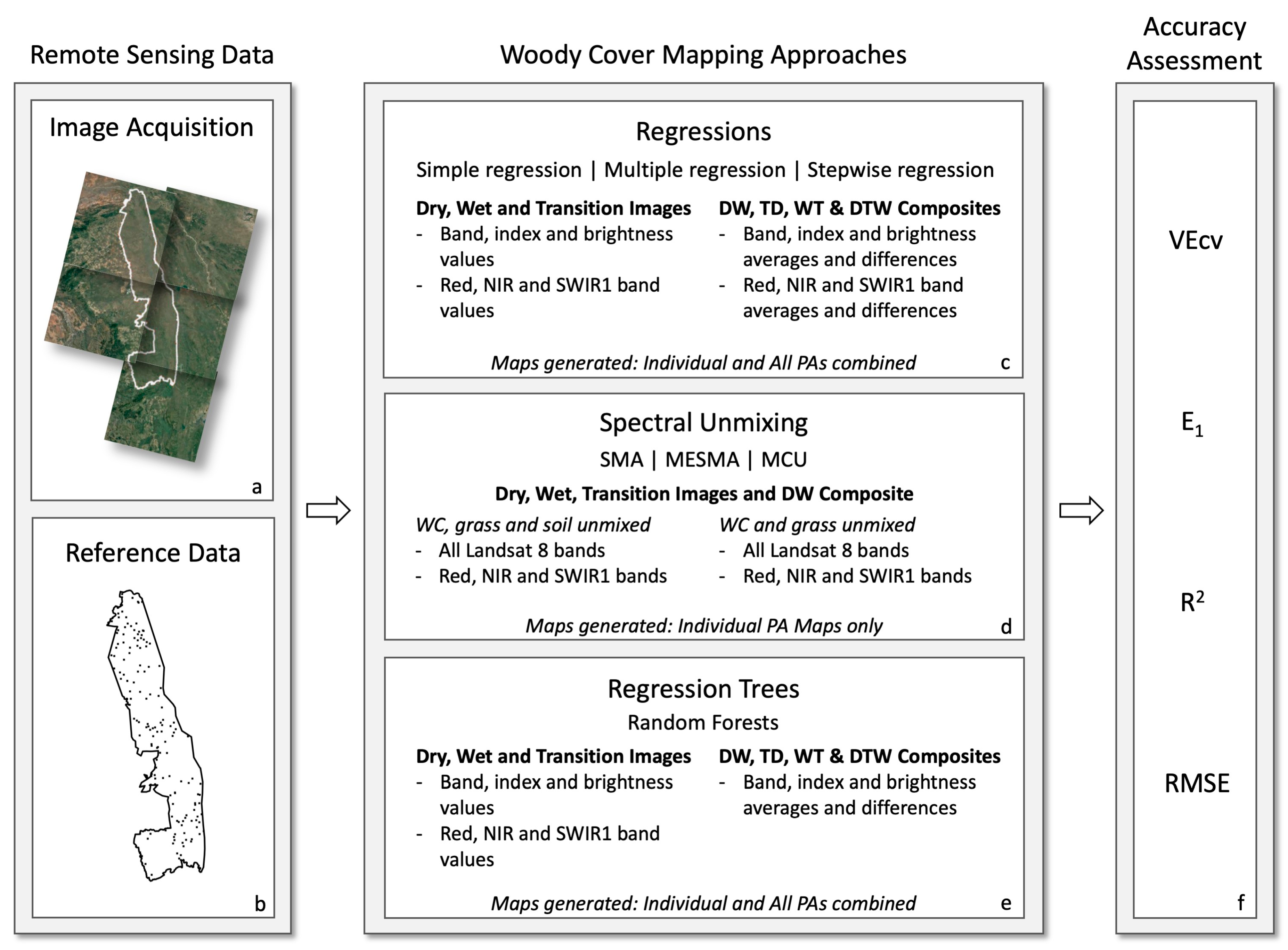
2.2. Remote Sensing Data

2.2.1. Reference Data

To train our approaches and assess the accuracy of the resulting maps, we generated WC reference data using VHR imagery available through Google Earth (Figure 2)—a practice that is increasingly common in broad-scale studies [54,55,56,64,65,66]. We note that in our maps and reference data, we mapped crown cover (the vertically projected area occupied by a tree crown), not canopy cover (crown cover minus intra-canopy skylight). We assume the globally derived relationship between canopy cover and crown cover (canopy cover = 0.8*crown cover) [37] holds in our study sites, allowing us to convert when necessary (e.g., VCF uses canopy cover instead of crown cover).

Previous studies mapped reference point landcover using a range of techniques, such as visual estimation [56,65], decision tree algorithms [64] and augmented visual interpretation using software such as CollectEarth [54,55,67]. In particular, CollectEarth uses VHR imagery from Google Earth and Bing Maps to compute helpful metrics (e.g., vegetation indices), then uses tens of user-classified sampling points within the reference image to estimate the spatial extent of each cover type.

Similar to CollectEarth, we developed a fast, semi-automated approach using VHR imagery from Google Earth. However, our approach mapped, rather than sampled, the complete extent of each cover type (code available in the online dataset: [68]). We downloaded VHR true color imagery from Google Earth (GE) using the RgoogleMaps package [69] in R [70], retrieving 180 × 180 m areas centered on one 30 × 30 m Landsat pixel (the reference point). We then mapped our perceived extent of WC, herbaceous cover (simply “grass”, hereafter) and soil cover of the 30 × 30 m reference point by manually thresholding image-derived metrics.

In our mapping, we took advantage of the fact that WC is predominantly darker than both soil and grass, thresholding pixel brightness (the sum of RGB values) to classify WC. When necessary, we adjusted thresholds to account for shadows that would have otherwise inflated WC values. In addition, when visually distinguishing WC from grass was a challenge, we assumed that objects with shadows were WC. We also used any on-the-ground photographs available through GE, along with our own on-the-ground experience in African savannas, to further inform our mapping. If we could not confidently distinguish a reference point’s WC, or if brightness thresholding failed to do the same—both of which were common when defoliated WC was present—a new reference point in a different location was automatically generated.

After WC, the remaining grass and soil were classified using pixel brightness in conjunction with the Green-Red Vegetation Index (GRVI) (

Table 2. Equations for indices used in this study. Color names refer to the corresponding image band.

Index	Equation*
Green-Red Vegetation Index (GRVI)	$\frac{Green-Red}{Green+Red}$
Normalized Difference Vegetation Index (NDVI)	$\frac{NIR-Red}{NIR+Red}$
Soil Normalized Difference Index (SNDI)	$\frac{Red-\left(NIR+SWIR1\right)}{Red+\left(NIR+SWIR1\right)}$
Soil Adjusted Total Vegetation Index (SATVI)	$\frac{SWIR-Red}{SWIR+Red+L}(1+L)-\frac{SWIR2}{2}$
Modified Soil Adjusted Vegetation Index (MSAVI2)	$\frac{2NIR+1- \sqrt{{\left(2NIR+1\right)}^2-8\left(NIR-Red\right) }}{2})$

* Spectra names (Red, Green, NIR etc.): Landsat reflectance bands. L: the soil adjustment factor – a constant set at 0.5 [72,73].

) [71], an index that exploits the red and green spectral differences between green vegetation and soil. However, we found that the GRVI threshold could often be left static (ca. −0.1), with only brightness threshold adjustment needed. We mapped a minimum of 100 reference points in each PA, increasing the number when densities fell below one point per 200 km², altogether mapping 1330 reference points. All the points were in cloud-free positions in the Landsat imagery. We then randomly subset the data, splitting it into PA-specific training (70% of points) and testing data (30%).

2.2.2. Landsat Image Collection and Processing

We collected Landsat 8 Tier 1 Surface Reflectance imagery for 2016 using Google Earth Engine (Figure 3) [74]. Google Earth Engine (GEE) utilizes the computational capabilities of Google to enable researchers to access and process the Landsat archive. We used GEE to select, preprocess, and download imagery, as well as carry out a subset of our mapping approaches (described below). However, we limited our exposure to any potential change or loss of services from GEE, such as Google’s 2018 decision to phase out their “Fusion Table” data type [75], by carrying out most of our mapping outside of GEE. We selected relatively cloud-free imagery (< 30% cloud cover over PAs in wetter regions (SEL, SER, MAR, RUA, MUR, QUE); < 10% in drier regions (CHO, MPA, KRU, LIM, NLU, SLU) (Table 1)), and required all PA images within the same Landsat path to be from the same date. We then cloud masked the imagery and selected images we estimated to correspond with the wet, dry, and transition seasons. For each PA, the wet season image (Wet) was characterized as that with the highest mean Normalized Difference Vegetation Index (NDVI; Table 2) [76]; the dry season image (Dry) as that with the lowest NDVI; and the transition (Tran) as that with its mean NDVI closest to the midpoint between the Wet and Dry NDVIs, falling chronologically after the wet season and before the dry season. If no image met our requirements for the Tran image, we took the image closest to the NDVI midpoint, regardless of where it fell in the year.

The purpose of using three images was three-fold. First, by using the images individually, we aimed to identify the time of the year that led to the best maps of WC. Past studies attempting to map WC and/or biomass have used the dry season [52,77], while others have used the transition [78,79]–sometimes at the same sites [52,78]–with no consensus on the most accurate approach. The dry season is often selected because many woody species remain green, enhancing the difference between their spectral signatures and that of brown, senesced grass, thereby aiding mapping [80,81,82]. However, drier tropical and subtropical sites generally have more trees that drop all or a fraction of their leaves during the peak of the dry season (drought deciduous or raingreen) [83,84]. Therefore, we expected Tran images to outperform Dry images in the drier of our sites. Finally, we expected the Wet images, captured when both woody and herbaceous plants are photosynthetically active and therefore most spectrally similar, to yield the least accurate maps. The second reason we used three images was that, when stacked together into a single image or used to create summative statistics, we expected to increase map accuracies by capturing the phenological differences of woody and herbaceous vegetation, as done in similar work [56,85,86,87]. Third, we limited ourselves to three images to simulate the shortage we would likely encounter when mapping historical imagery.

Because many of the PAs spanned multiple Landsat paths and each additional path added significant time investment, paths that covered less than 10% of a PA were excluded. Adjacent PAs in the same path with imagery from the same dates were treated as a single PA (requirements only met by SER and MAR, hereafter together referred to as “SMR”).

In all, 105 individual Landsat scenes were selected. Images in the same path were subsequently mosaicked, yielding 45 images. We then masked all the images within each PA using the same PA-specific mask. Each PA’s mask was generated using the “pixel_qa” band provided with the Landsat data, and all but the pixels marked as “clear” were removed by the masks. The masks were combined across seasonal images, meaning masked areas in one image were masked in the others. This meant that sometimes large image fractions (approx. 15–20%) were removed, which is not ideal when creating a map. However, our objective was not to create contiguous images but was to produce images with identical data to test which seasons and approaches best predicted WC.

Finally, we clipped the images to 20-km buffers around each PA boundary, with the exception of the smallest PA, MPA, which we clipped to a 50-km buffer. The buffers allowed us to capture areas with 100% crown cover—areas often only available outside PAs and required in a subset of our approaches. All images were then downloaded from GEE (code available in the online dataset: [68]).

For the 70% of reference points serving as training data, we extracted Landsat reflectance values to serve as predictors of WC. For each point, we supplemented reflectance values with indices known or likely to have relationships with vegetation in semi-arid environments [50]: the Soil Normalized Difference Index (SNDI) [50], Soil Adjusted Total Vegetation Index (SATVI) [73], the updated Modified Soil Adjusted Vegetation Index (MSAVI2) [72] and NDVI [76] (Table 2). We also computed the visual brightness (mean of red, green and blue bands; hereafter simply “brightness”) of each reference point. We chose brightness because of the strong relationship it had with WC during reference point generation, as mentioned in Section 2.2.1 above. We then created an additional variable to contextualize the brightness within the landscape because, when we were creating the reference data, views of the larger landscape helped the user distinguish between grass and WC. In particular, a completely wooded pixel was often only distinguishable from a grass-dominated pixel when we viewed the larger landscape and saw all the brighter, grass-dominated pixels. To generate the contextualized variable, we computed the normalized difference between reference point brightness and PA mean reference point brightness. We refer to this as the brightness context (BC; Table S1).

In addition to the variables generated from single images, we created multi-image composite variables to incorporate phenology—a practice not novel to vegetation mapping [37]. The specific image composites were: Dry, Tran and Wet (DTW); Dry and Wet (DW); Tran and Dry (TD) and Wet and Tran (WT). The values for each composite’s variables were calculated by taking the mean and normalized difference of each single-image variable across images (testing showed the normalized difference had stronger relationships with WC than the simple difference). This doubled the number of variables in the composites compared to the single images. For example, while the Dry and Wet images each generated a single NDVI variable, the DW composite had two NDVI variables: the (1) mean and (2) normalized difference of the Dry and Wet NDVIs. However, the DTW composite presented a unique challenge: calculating the difference of three values (e.g., Dry NDVI, Wet NDVI and Tran NDVI). We therefore computed the DTW differences by subtracting the normalized differences of the WT composite from the DW (Table S1). This metric had a distinct phenological meaning. Assuming the date of the Tran image was between the Wet and Dry, a value of zero meant all changes in the variable occurred early (between the Wet and Tran images)—likely representative of the early senescence of a grass-dominated pixel. As more of the total change occurred after the Tran image (i.e., the late season senescence of woody cover), the value exponentially approached 1 or −1, depending on the direction of the variable change moving from the wet to the dry season (e.g., for NDVI, which decreases across the seasons, the DTW difference metric approaches −1). For simplicity, we use “difference” to describe the difference metrics of all the composite images, even though all but DTW use the normalized difference.

Across the single images and composites, these steps generated 132 variables (Table S1). Hereafter, we refer to these data collectively as the “reflectance data.”

2.3. Mapping Woody Cover

We mapped WC using seven techniques falling under three general approaches: linear regression, spectral unmixing, and regression trees (Figure 3). To incorporate their nested structure, we refer to these as “sub-approaches” and “approaches,” respectively. Because all the approaches were not available in a single software package, we worked across multiple programs. Further, not all approaches used all the possible variables when those variables did not improve results and/or caused inputs to exceed the capacity of most modern computer systems, thereby limiting their adoption (see Section 2.3.2). The programs and approaches are described below, with detailed procedures and code provided in the online dataset: [68].

2.3.1. Linear Regression

We used linear regressions [88] to identify any consistent relationships between the reflectance data and WC. All regressions were carried out in R [70]. We expected maps generated using linear regression would form baseline accuracies compared to the other, more complex, approaches.

We conducted regressions using three sub-approaches. In the first, all 132 reflectance data variables were regressed independently against WC (simple linear regression). In the second, we used the red, near infrared (NIR) and first short-wave infrared (SWIR1) bands together in multiple regression (for the composite images, we did separate regressions using the means (1) and differences (2) of the red, NIR and SWIR bands). We refer to these as the “RNS” bands/regressions. We chose the RNS bands because they capture the spectral signature of vegetation, hence their widespread use in vegetation indices [50,72,73,76]. Third, we conducted forward stepwise regressions (STEP) to identify novel relationships that might warrant further investigation. To avoid overfitting the models and multicollinearity between variables, we only added variables with high levels of significance within the new model (p-values below 0.05) and low collinearity (R² < 0.6).

We carried out the regressions in individual PAs to derive PA-specific relationships, then with all PAs combined (“ALL”) to derive regional relationships. Altogether, the simple, RNS and STEP regressions yielded 1800 regression models. We applied the models to their respective PAs, then applied the ALL-derived, regional models to the individual PAs to quantify the local accuracy of the regional models.

2.3.2. Spectral Unmixing

Spectral unmixing, which some have shown outperforms linear regression in savanna WC mapping [89], is based on the premise that pixel reflectance is an area-weighted, linear combination of the landcovers within each pixel [90,91]. Spectral unmixing, then, uses the reflectance values of each individual cover type—values referred to as “endmembers”—to unmix, or back-calculate, the fractional coverage of each land cover type within a pixel. A unique feature of this approach, compared to other approaches used here, is that field-based measurements are not required—all values can come from the image being unmixed [92]. This means unmixing can be done on historical imagery where no ground truth or reference data is available, which made it particularly attractive for our goals. The challenge, however, is selecting endmembers that (1) have only the target land cover in the pixel and (2) best summarize a land cover’s spectral variability.

Multiple unmixing sub-approaches have been developed with their own method of endmember selection. We selected three common sub-approaches and used each to unmix WC, grass, and soil fractions in each image. The first sub-approach, spectral mixture analysis (SMA) [45,90,91,93], relies entirely on the user to identify the best endmembers. We selected endmembers with the minimum, maximum, mean, and median brightness values (sum of all bands). Separate SMAs were ran for each endmember in GEE using the “unmix” function [74].

The second sub-approach, Multiple Endmember SMA (MESMA) [94], builds upon SMA by allowing multiple endmembers within a single class, instead of only one, affording the classifier more flexibility and greater mapping accuracies [95]. MESMA selects endmembers by running individual SMAs with every possible combination of endmembers, while also allowing the number of classes to vary [94]. It then retains, on a per-pixel basis, only those results from the best-fit model. In other words, a MESMA result is a mosaic of the best-fit SMAs. The MESMAs were run in ENVI (Harris Geospatial Solutions, Boulder, CO) using the ViperTools add-on [92].

Even though MESMA can take as input all potential endmembers, the evaluation of all the models (>200,000 in many cases) required significant processing time. To minimize this, Roberts et al. [92] recommends screening out spectrally similar endmembers by examining whether the endmembers formed clusters, then selecting the endmembers that best represented each cluster. To do this, we used metrics built into ViperTools: Endmember Average RMSE (EAR) [96], Count-based Endmember Selection (COB) [97] and Minimum Average Spectral Angle (MASA) [98]. We used the metrics according to the methodology suggested by Roberts et al. [92] (p.44), selecting endmembers with the lowest EAR within each COB-identified cluster, or the lowest MASA when COB failed to identify any clusters. We referred to this as the EMC (EAR-MASA-COB) selection method. The EMC method yielded 1–5 endmembers for each class.

In a separate method, after testing multiple selection criteria, we found selecting endmembers from each class using the minimum, maximum, and mean brightness values (sum of all bands) yielded the best results. We referred to this as the HML (high-middle-low) selection method.

Altogether, these endmember selection methods yielded ca. 20–40 models per MESMA—a significant reduction from the thousands the full suite of endmembers generated. To ensure the reduction in models was not having a detrimental effect on the accuracy of the MESMA results, we ran preliminarily tests using the full suite of endmembers versus our subsets and found no significant difference.

The third unmixing sub-approach, Monte Carlo Unmixing (MCU) [53,99], is similar to MESMA in that it allows multiple endmembers within a class. However, whereas MESMA selects results based on best-fit models, MCU iteratively draws random selections from the pool of endmembers, running an SMA for each. MCU then reports the mean and standard deviation of all the results as the final result. However, the final result is sensitive to the number of iterations; with too few iterations, different MCUs can yield very different results. Therefore, the stability of the final result depends on the number of iterations. Others achieved stability after 30 iterations [100]. Because we had several sites with multiple images per site, all of which might achieve stability at a different number of iterations, we set the number of iterations at 300—a number we assumed would achieve stability in all locations. We wrote and ran our own MCU function in GEE utilizing the “unmix” function. The code for the MCU function is available in the online dataset [68].

Unlike the regressions, which used the reflectance data described in Section 2.2.2 (i.e., point data) to train and test models, unmixing used entire Landsat images. This, in combination with the fact that MESMA was not automatable, led to marked increases in user input and computational demands. Consequently, we limited the number of images we unmixed, along with the number of bands/variables in each image. We created DW composites with the Dry and Wet image bands stacked into a single image without any of the additional bands/variables described in Section 2.2.2. The same applied to the Dry, Wet, and Tran images: they only contained the original Landsat bands. However, unlike the regressions, the unmixing approaches utilized the full suite of bands available from Landsat 8: bands 1–7 (visible, near infrared and short-wave infrared bands) and 10–11 (thermal bands). While earlier Landsat satellites do not have bands 1, 10, and 11 we found that including these bands substantially increased accuracies, while bands representing the vegetation indices did not. We did not test all the possible additional bands and combinations because of the amount of time this would have required.

Because linear mixture models can produce results outside the range of 0–1, all the unmixing methods allow the user to constrain the results to stay within the 0–1 range. Depending on the software, we found that constraining the results caused pixels to be removed (ViperTools) or forced to zero or one (GEE)—something we could do independently in post-processing. Therefore, we chose not to constrain the values. In addition, ViperTools had the option to constrain candidate models based on their RMSE and residuals, and GEE to constrain the unmixed values to sum to one. We set the RMSE constraint to 0.1 (effectively unconstrained) and left the other two unconstrained to avoid differences across unmixing methods.

As an alternative to constraining results in the individual software, we extracted mean mapped WC values from the WC (${\overline{\mathrm{WC}}}_{\mathrm{WC} }$) and grass (${\overline{\mathrm{WC}}}_{\mathrm{grass}})$ endmember pixel locations, which were meant to have 100% and 0% WC, respectively. We then normalized the unmixed values (${\mathrm{WC}}_{\mathrm{i} })$ following Equation (1):

$${WC}_{\mathit{normalized}} = \frac{{WC}_{i }-{\overline{WC}}_{\mathit{grass}}}{{\overline{WC}}_{WC }-{\overline{WC}}_{\mathit{grass}}}$$

(1)

This was meant to preserve more of the relationship between the unmixed values and the reference data—a relationship that was lost using the software constraints described above if all unmixed values were negative or over 1, which was not uncommon. However, normalization still left some mapped values outside the 0-1 range, and it was at this point that we set negative values to zero and high values (>1) to one.

For each approach, in addition to unmixing WC, grass and soil, we also unmixed only WC and grass to test if accuracies improved when unmixing only these, the two most similar cover types. As in the regressions, we also ran a subset of approaches using only the RNS bands. However, unlike the regressions, we did not combine all the PAs and unmix them as a single PA, nor use such a model to map individual PAs.

2.3.3. Regression Trees

Regression trees, unlike the other methods used here, are capable of handling non-linear relationships between landcover types and their reflectance—a situation which is particularly common when mapping at regional to global scales [38]. Accordingly, during the development of VCF, which used a coupled, regression tree and linear regression approach, Hansen et al. [101] found their approach outperformed spectral mixture analysis. We expected our regression tree approach to do the same.

However, we did not attempt to replicate the VCF approach, which used stepwise regressions at the regression tree nodes to smooth the outputs, along with variables derived from MODIS bands not available in Landsat imagery. Instead, we used another regression tree approach, Random Forest (RF) [102]. RF has become a popular and effective procedure for mapping WC in savannas [103,104,105], along with regional-to-global scale land cover [106,107,108,109]. RF draws random samples from a dataset of predictor and response variables using bootstrap aggregation to initiate a regression tree. RF then divides the data based on variance, creating branches with the smallest possible intra-subset variance at each split. However, instead of considering the entire subset at each split, RF uses a random selection of predictor variables to determine the split. This process is repeated to generate a “forest” of different regression trees. Once all trees are grown, a predicted value is calculated as the mean prediction of all the regression trees.

We performed the RFs in R using the randomForest package [110] and the reflectance data described in Section 2.2.2. The RFs used the entire set of predictor variables available for each image. Each RF was set to grow 500 trees and a set number of variables were randomly selected at each split: seven (out of 12 available variables) for the single-season images and seven (out of 24) for the composite images. We set the number of variables after we ran an optimization process across all the PAs that showed including more variables did not significantly improve accuracy—a threshold we sought in order to avoid overfitting the models. Like the linear regressions, the RFs were trained and applied to their respective PAs (including ALL), with the ALL-derived models also applied to the individual PAs.

2.4. Accuracy Assessment

We assessed the accuracy of the WC results from each mapping method using the variance explained by predictive models based on cross-validation (VEcv) (

Table 3. The names and equations of accuracy measures used in this study.

Accuracy Measure	Equation*
Variance Explained (VEcv)	$\left(1-\frac{{{\displaystyle \sum }}_1^n{\left(O_i-P_i\right)}^2}{{{\displaystyle \sum }}_1^n{{(O}_i-\overline{O})}^2}\right)100 (\%)$
Coefficient of Determination (R2)	$\left(1-\frac{{{\displaystyle \sum }}_1^n{\left(O_i-F_i\right)}^2}{{{\displaystyle \sum }}_1^n{{(O}_i-\overline{O})}^2}\right)100 (\%)$
Legates and McCabe’s (E1)	$\left(1-\frac{{{\displaystyle \sum }}_1^{\mathrm{n}}{|O}_i-P_i|}{{{\displaystyle \sum }}_1^{\mathrm{n}}{\left|\right(O}_i-\overline{O}|}\right)100 (\%)$
Root Mean Square Error (RMSE)	$\sqrt{\frac{{{\displaystyle \sum }}_1^n{(O}_i-P_i{) }^2}{n}}$

* O_i: the observed value; P_i: the predicted value; F_i: the fitted value from regressing predicted and observed values; n: the number of observations.

) [111]. VEcv and equivalent measures such as the G-statistic [112] and Nash-Sutcliffe efficiency [113] closely resemble the coefficient of determination (R²; Table 3). R² measures the proportion of the observed variance that is predictable from an independent variable (in this case the predicted values). However, in model validation, we are not interested in the ability of predicted values to predict observed values; we are interested in how well predicted values match the observed values. VEcv was developed for the latter case. It does this by directly comparing the observed values to the predicted values, i.e., a 1:1 line; rather than compare values to a fitted regression line, as R² does. In this way, VEcv is also similar to root mean square error (RMSE; Table 3). Beyond combining the utilities of R² or RMSE, VEcv values below zero correspond to instances where the mean of the observed values better predicts the observed values than the model being evaluated—something demarcated by neither R² nor RMSE. This means that while VEcv generates negative values that can appear meaningless, it is important to remember that the model producing a negative score could have a R² of 1.0 if it exhibits errors that can be perfectly predicted using the observed data. In such a case, RMSE would be required to show the model was flawed. Therefore, when a single metric is needed to rank performance across models, VEcv is superior and we use it for that reason. However, we recognize that most studies have used R² and RMSE and we include R² and RMSE values where we felt it would aid comparisons with other studies.

In addition to VEcv, we used Legates and McCabe’s efficiency (E1) (Table 3) [114] as a secondary measure of model accuracy. Whereas model errors are squared in the VEcv equation, E1 takes their absolute value, thereby quantifying the percentage of the sum of absolute differences explained by the model. Like VEcv, E1 reports accuracy as percentages, with 100% corresponding to an exact match and values < 0% denoting situations where the mean of the observed values is a better predictor of the observed values than the model. However, because VEcv uses squared errors, it is the more sensitive measure. For this reason, we primarily used VEcv and only utilized E1 if we needed to differentiate models with similar VEcv scores, as suggested by Li [111].

We assessed the accuracy of the maps using the withheld testing data/points (30% of reference points). The same PA-respective testing points were used across all maps. We compared the accuracies across approaches and sub-approaches, then across seasons and variables, and finally present the best approaches both overall and for each PA. We used ANOVAs and post-hoc Tukey honest significant different (HSD) tests to compare accuracies across approaches and sub-approaches. To compare seasons and variables, we used repeated measures ANOVAs and HSD. Throughout, we also evaluate the relationship between the Landsat-rescaled VCF tree cover dataset [115] and WC. We refer to both VCF [37] and the Landsat-rescaled VCF [115] as “VCF” and assume that for our purposes there are no meaningful differences between the two. This is not an accuracy assessment of VCF, which monitors woody vegetation >5 m, while our reference data monitor all woody vegetation, regardless of height. However, we included VCF to demonstrate the amount of woody vegetation excluded by VCF in these systems and assess whether VCF might be used to predict WC (i.e., whether an adjustment factor can convert VCF tree cover to WC).

2.5. Post-Processing

Some post-processing of the accuracy assessment data was necessary. Overall, models trained and applied to individual PAs and all the PAs pooled together created 4842 WC maps with accuracies ranging from a high VEcv of 91.1% down to scores below −1000%. While negative VEcv scores are to be expected, some appeared so low they might bias our final results. Normal outlier analysis removed more points than we felt appropriate, so instead we ranked and plotted all 4842 map accuracies in search of an inflection point, i.e., where gains in accuracies from map to map become relatively consistent. We found this point around a VEcv of -500% (Figure S1). We removed maps below this threshold from further analysis, eliminating 157 maps (~ 3% of the total number of maps). The majority (147) of these were produced using spectral unmixing. The remaining were from regressions.

3. Results and Discussion

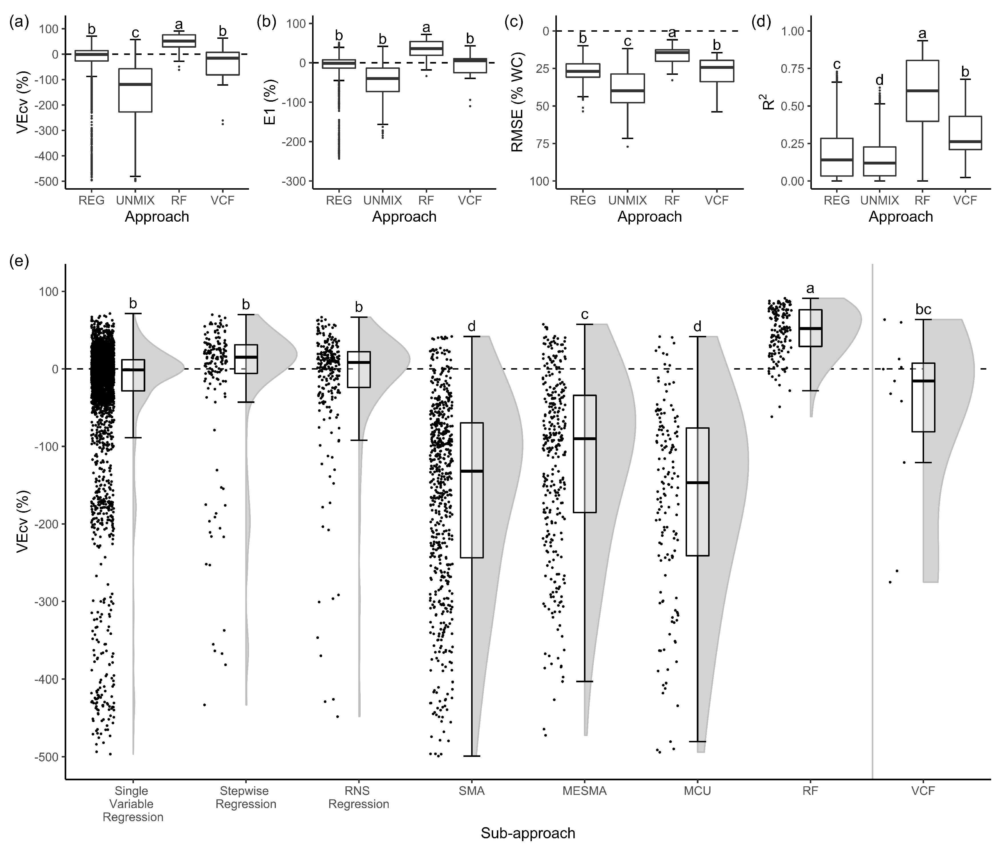
3.1. Evaluation of Accuracy Measures

Because VEcv is not a commonly used measure, we first compared approach accuracies using VEcv, E_1, RMSE and R² (Figure 4a–d). While all the measures found RF significantly outperformed the others, R² gave VCF scores significantly higher than the regressions and unmixing approaches, while VEcv, E₁ and RMSE did not (Figure 4d). As outlined in Section 2.4, this is likely due to the fact that R² is not a measure of model accuracy while the other measures are, including RMSE (Table 3) [111]. Because VEcv produced results similar to those using E₁ and RMSE, and is the most sensitive measure of accuracy, we used it for the remaining analyses.

3.2. Best Approaches and Sub-Approaches

Across both the approaches and sub-approaches, RF significantly (p < 0.001) outperformed the others, rarely scoring below zero, with a VEcv mean and standard deviation of 49.0 ± 30.8% (Figure 4a,e).

Spectral unmixing underperformed the other approaches (VEcv mean and standard deviation of −148.8 ± 123.0%; Figure 4a). We expect spectral unmixing was limited due to the fundamental challenge of choosing endmembers. While it might be possible to accurately define endmembers across a relatively small area, when the study area expands, so does the spectral variability within each landcover type, making endmember definition more of a challenge. For this reason, successful applications of spectral unmixing often include a regional component in endmember selection [116]. We decided adding a regional component to our endmembers was infeasible: candidate endmembers were often scarce within the PAs, let alone areas within the PA. Other successful applications of spectral unmixing have been aided by additional data, such as the increased number of bands and finer spectral resolution of hyperspectral imagery and/or airborne lidar which help differentiate cover types [117]. Here we were limited to Landsat’s relatively coarse spectral resolution (9 bands). Though including variables identical to those available to RF and the regressions might have improved accuracies, this was not possible due to computational limitations. Further, this would have required the removal of bands 1, 10, and 11 – bands whose testing showed improved results while the vegetation indices did not.

Among the unmixing sub-approaches, MESMA significantly outperformed MCU and SMA. We attributed this to the fact that MESMA uses a more advanced approach to selecting the best endmembers for each pixel. Because of the overall poor performance of the spectral unmixing approach, we did not evaluate the effects of the different settings within the models (e.g., unmixing woody cover and grass versus unmixing woody cover, grass and soil).

Regressions significantly (p < 0.05) outperformed the spectral unmixing sub-approaches (Figure 4a). While no regression sub-approach significantly outperformed the others, stepwise regression, with its ability to add significant predictor variables, performed better on average (Figure 4e). The regressions did not significantly outperform VCF in an HSD test, likely due to the limited number of VCF data points (n = 11).

3.3. Evaluation of Seasonal Images

Unlike the approaches and sub-approaches, both within and across PAs, no season significantly outperformed all the others (Figure 5;

Table 4. Best seasons, approaches, and models as measured by VEcv (%). The best locally derived model refers to those trained using reference data from the respective PA only. The best overall model is that with the absolute highest accuracy, regardless of the source of the training data. The best general model is the single model that did best on average across all the PAs. Model naming structure: Approach - source of training data - image season - variables used in model. We list the source of the training data only when it was ALL—the combination of all the PAs in this study—otherwise the source is the PA itself. Similarly, only models that used individual variables (i.e., regressions; “REG”) list those variables. Standard deviations are given where accuracies are mean values; otherwise, values are the accuracy of the single map produced by the model. Because we did not apply the unmixing approach to all image combinations (only DW), we excluded unmixing results from the best season evaluation, resulting in higher than otherwise expected mean accuracies.

PA Abbr.	Best Season		Best Approach		Best Locally Derived Model		Best Overall Model		Best General Model†	VCF
	Season	VEcv	Approach	VEcv	Model	VEcv	Model	VEcv	VEcv	VEcv
MUR	DTW	46.8 ± 24.5	RF*	79.3 ± 8.6	RF - WT	78.4	RF - ALL - DW	88.6	88.6	60.0
MPA	Dry	15.6 ± 16.6	RF*	55.7 ± 21	RF - WT	50.1	RF - ALL - TD	78.1	76.5	−120.7
QUE	Dry	−1.7 ± 20.3	RF*	55.4 ± 27.6	RF - DW	52.0	RF - ALL - DW	91.1	91.1	63.6
SMR	DTW	10.8 ± 18.5	RF*	−2.8 ± 21.7	MESMA EMC TG - Dry	42.1	MESMA EMC TG - Dry	42.1	15.9	12.7
RUA	WT	1.2 ± 23.9	RF*	46.1 ± 25.4	RF - DW	35.6	RF - ALL - DW	76.3	76.3	−0.2
SEL	Tran	37.1 ± 19.5	RF*	67.3 ± 16.3	REG - TD - Mean NDVI & Band 5 Normalized Difference	58.3	RF - ALL - DTW	86.2	80.2	−32.1
NLU	Tran	20.6 ± 10.4	RF*	53.7 ± 30.1	REG - TD - Mean NDVI	40.1	RF - ALL - DTW	87.1	79.7	−2.1
SLU	Tran	35.5 ± 19.6	RF*	67.3 ± 18.6	RF - WT	65.8	RF - ALL - DTW	86.6	77.6	−15.6
CHO	Tran	29.9 ± 14.1	RF*	56.2 ± 18.5	REG - DTW - Mean NDVI	46.1	RF - ALL - DW	76.8	76.8	−260.6
LIM	TD	23.2 ± 11	RF*	41 ± 27.2	REG - Dry - Brightness & NDVI	40.8	RF - ALL - Dry	75.4	71.5	−275.1
KRU	Dry	0.7 ± 18.9	RF*	21.1 ± 31.2	REG - Dry - MSAVI2	29.4	RF - ALL - DW	53.4	53.4	−41.6
ALL	Tran	15.3 ± 10.5	RF*	46.2 ± 4.7	RF - ALL - DTW	51.1	RF - ALL - DTW	51.1	49.5	−7.9

* Seasons, approaches and models that significantly (p < 0.05) outperformed their counterparts. Significance testing was carried out using two different measures depending on the comparison: Repeated Measures ANOVA (best season) and simple ANOVA (all others).^† RF - ALL - DW was the best general model.

). DTW did the best on average (VEcv mean and SD of 16.6 ± 23.8%) and significantly outperformed the Dry, Wet, and DW images, with the Wet image performing the worst (6.5 ± 24.9%). DTW did not significantly outperform TD, WT, or Tran. This confirmed our expectation that the image with the most information (DTW) would do the best, while the Wet season image, captured when WC and grass are most spectrally similar, would do the worst. Meanwhile, the Tran image was included in all the best performing images (DTW, TD, WT, and Tran). We also found that Tran was the best image when all PAs were combined (see “ALL” in Table 4). These findings suggest the Tran image is critical to mapping WC. Indeed, all the images with the lowest scores did not contain Tran (Dry, Wet, and DW) and Tran significantly outperformed both Dry and Wet, making Tran the best option if a user were going to use only a single image in a new site.

The best image for each PA varied and, like above, no image significantly outperformed all the others within a single PA (Table 4). However, unlike above, most of the best images in the PAs were something other than DTW (Table 4). Instead, Tran was most often selected as the best image and was included in the majority (9 of 12) of the PAs’ best images (i.e., DTW includes Tran). This provided further evidence that the Tran image is critical to mapping savanna woody cover, likely capturing WC and grass at their most spectrally dissimilar point, when WC is still green and grasses have senesced.

We tested whether we could generalize the best image for a PA based on the PA’s average woody cover, mean annual precipitation (MAP) or precipitation seasonality (WorldClim bioclimatic variables #12 & 15, respectively). For instance, we expected one image might do best in drier PAs and another in wetter PAs. However, MAP and precipitation seasonality had no relationship with accuracies. Meanwhile, WC had a positive relationship with accuracies, but the relationship existed across all the images (Figure S2). While this meant woodier PAs are likely to have the most accurate maps, it also meant that, like MAP and seasonality, the WC of a PA cannot be used to determine the best image.

While no image across or within PAs significantly outperformed the others and the PA characteristics we tested could not be used to predict a best image, it was also encouraging: the findings also suggest one could use any of the seasonal images or composites – whichever available. The notable exception to this was the Wet image. The Wet image had the lowest average score across the PAs, never appeared as a PA’s best image, nor was it ever used alone in any of the best models (more on models in Section 3.6; Table 4).

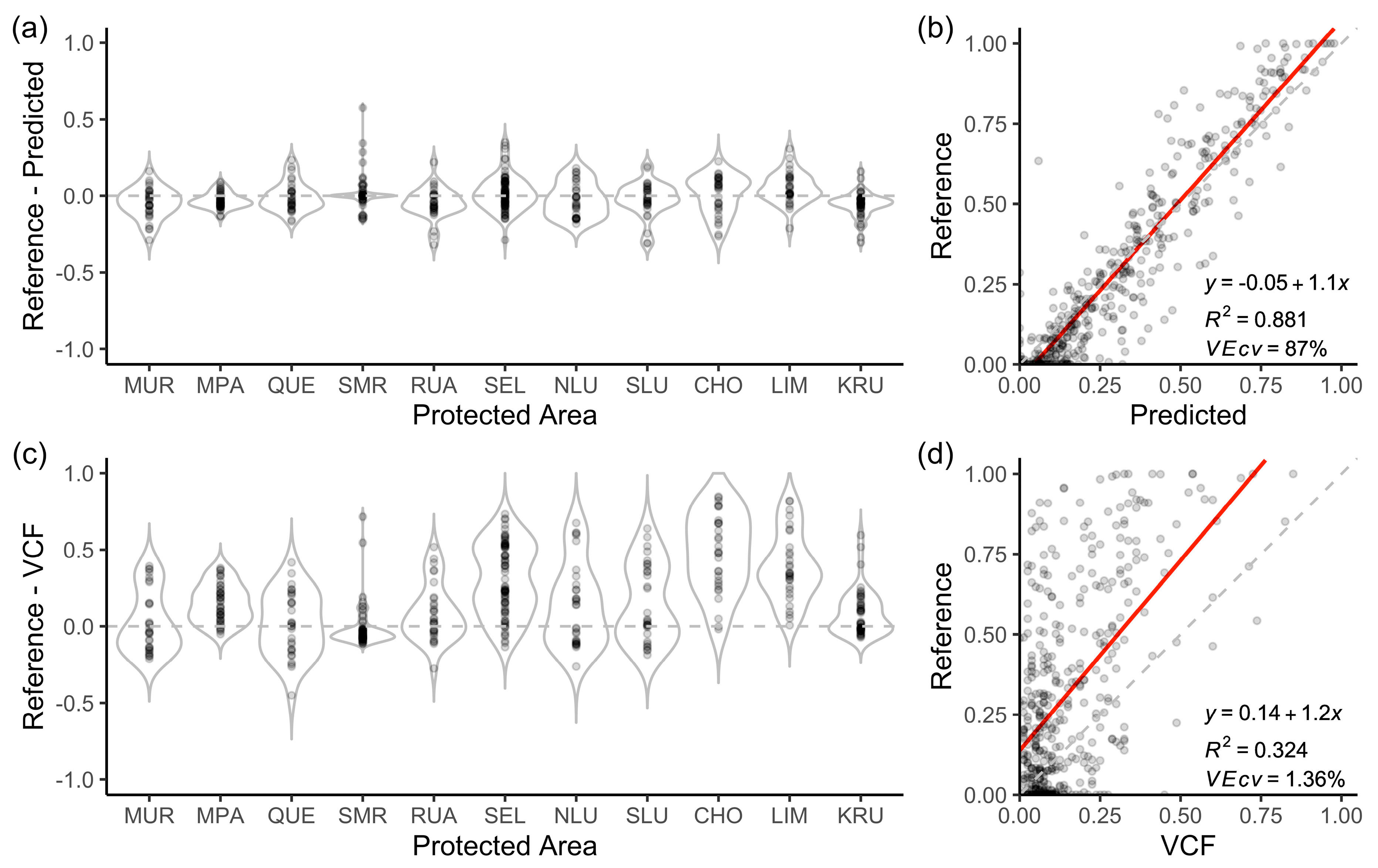
3.4. Evaluation of Protected Area Accuracies

Among the individual PAs, MUR had significantly (p < 0.05) higher scores than all the other PAs (VEcv mean and SD of 41.7 ± 23.6%; Figure 5). RUA, KRU, and QUE all produced the least accurate maps (average accuracies amongst the three were not significantly different). Of them, QUE had the lowest average score (−9.1 ± 33.7%). Like the images, we tested for relationships between PA accuracies and MAP, precipitation seasonality or average woody cover. Like before, we found a positive relationship (significant) with PA woody cover (Figure S3) but no relationship with MAP or seasonality. Again, this suggests woodier PAs are easier to map while a similar relationship does not extend to MAP or seasonality.

3.5. Evaluation of Variables

Across PAs and seasons, we found that regression models using RNS, NDVI, and BC performed the best (average accuracies amongst the three were not significantly different), with VEcv means and standard deviations of 23.7 ± 20.5%, 22.9 ± 23.9%, and 21.5 ± 21.5%, respectively. The variables significantly outperformed all the other variables, except Band 4 (red), which NDVI and BC did not significantly outperform. The variables with the lowest scores were SNDI, SATVI and Band 5 (−4.7 ± 12.1%, −0.6 ± 32.5%, and −0.4 ± 12.4%, respectively).

We also tested for the image-specific variable that best predicted WC across all PAs. We found this to be the mean NDVI of the TD composite (Figure S4; VEcv: 29.1 ± 25%). While it did not have an average score significantly higher than all the other variables, it was the only variable to significantly outperform some of the other variables (47 out of 143). Most of these (37 of 47) were composite image variables derived using the normalized difference, suggesting the mean was the better statistic to use for these images. We tested this and found the mean significantly (p < 0.001) outperformed the variables derived using the normalized difference, with respective scores of 13.0 ± 23.3% and −5.2 ± 22.7%. Therefore, while the variables using the normalized difference might add some explanatory power to WC models, it is likely minimal.

Stepwise regression revealed no novel, consistently strong (VEcv > 50%) relationships between any combination of variables and WC across the PAs. However, NDVI and BC were the most commonly selected variables across the 84 total stepwise regressions: NDVI was selected in 29, and BC in 17. When we pooled all the PAs’ data together as if they were single PA, NDVI was not selected in any of the regressions. Instead, the stepwise regressions selected BC alone or in combination with other variables in five of the seven regressions (one regression per image). Accuracies ranged from 18.2 to 24.9%. These findings suggest that as the mapped area expands, relationships between NDVI and WC break down, while for BC, which simply quantifies how bright a pixel is in relation to its surroundings, they remain relatively robust.

3.6. Best Models

The main objective of our work was to develop a single, accurate model for mapping WC. We first evaluated the best models trained and tested within the individual PAs (“Best Locally Derived Model” in Table 4). Across the 12 PAs (including ALL), most of the best models (11 of 12) were either regression- or RF-based, and several utilized NDVI. However, there was no clear pattern between the models. We then expanded the pool of models to include those trained using data from all the PAs combined (“Best Overall Model” in Table 4). Only one of the locally derived models was the best overall model for the PA: the SMR-derived MESMA that unmixed only WC and grass (TG) using the EMC endmember selection method and the Dry image (MESMA EMC TG – Dry). For all the other PAs besides SMR, the best overall models were RF models trained using data from all the PAs combined. When we expanded the comparison to include all RF models (not just the best), those trained using data from all the PAs and tested in the individual PAs significantly (p < 0.001) outperformed those trained and tested in a single PA (VEcv: 67.7 ± 23.3% versus 30.5 ± 27.4%; R²: 0.76 ± 0.16 versus 0.42 ± 0.19; RMSE: 12.5 ± 2.6% WC versus 19.5 ± 5.2% WC). This implies researchers can use training data from many savanna sites, even those hundreds of kilometers away, to improve models for a single site. This might be particularly helpful for researchers with limited data for their site. This finding also suggests that PAs share WC-reflectance relationships that a single model could use to accurately map WC across space and time.

We also tested for the model that produced the highest average accuracy across PAs (‘Best General Model’ in Table 4). This model was RF-ALL-DW: an RF model using training data from all the parks (ALL) combined and the DW image. Compared to the best overall models for each PA, RF-ALL-DW did not cause a significant decrease in accuracy: average accuracy across the parks fell 4.9 percentage points, from VEcv values of 76.5 ± 15.4% to 71.6 ± 20.8% (p = 0.063). We note that when all the PAs were combined (i.e., the testing data from the different PAs was combined) and mapped as a single PA (“ALL” – last row of Table 4), the RF-ALL-DW model did not produce the best results – instead, the best model was RF-ALL-DTW. The difference is attributable to the fact that we ranked each candidate model based on its average accuracy across all the PAs, not based on its ability to map all PAs as one (like R², the average VEcv of different datasets will not equal the VEcv when those data are pooled and evaluated as one).

Last, we tested which model performed best on average across all the PAs when only using training data from the individual PAs. In other words, we wanted to know the model that was most likely to perform well when mapping WC somewhere outside our list of sites using only training data from the new site. Like above, this model proved to be a RF using the DW image (RF-DW).

Both within and across PAs, while the best models did significantly outperform many of the other models, they did not significantly outperform them all (Table 4). This, in combination with the similar finding for the images, suggests that when attempting to map WC through the Landsat archive, researchers can be flexible in their year-to-year image and model selections. For example, if a researcher wanted to produce a map for SEL, the best model to use would be the RF-ALL-DTW (VEcv of 86.2%). But if the Wet image was not available, then the next best model, RF-ALL-TD (VEcv of 85.4%), would result in what is still an accurate map with an accuracy that is not significantly lower than RF-ALL-DTW. The same would apply if only the Tran image were available: RF-ALL-Tran would produce an accuracy of 84.5% (see the online dataset for a complete list of model accuracies). Besides providing flexibility year-to-year, these findings suggest areas with cloud cover in one image could be filled using WC values derived from the next best cloud-free image—something we did not attempt to do here.

3.7. Map Comparisons

We compared the accuracies of both the maps produced by the best overall models (“Best Overall Model” in Table 4; Figures S5–S13) and VCF (Figure 6 and Figure 7). For VCF, in one respect this was a simple demonstration of the difference between tree cover and WC, but it was also a true measure of VCF error where VCF exceeded WC (WC includes tree cover, therefore VCF values that exceed WC are true overestimates).

Overall, our maps had a significant (p < 0.001) and strong relationship with WC (combined VEcv = 87.0%, R² = 0.881; Figure 6b), while VCF had a significant (p < 0.001) but relatively weak relationship with WC (combined VEcv = 1.36%, R² = 0.324; Figure 6d). Our maps overpredicted WC in areas of sparse WC and underpredicted in woodier areas (Figure 6b), while VCF was mostly below WC but exceeded WC (true errors) at 139 of 421 testing points, mostly in sparsely wooded areas (<~10% WC; Figure 6d). Wald tests showed these biases were significant (the regressions between WC and our maps and VCF differed significantly from 1:1 lines). However, when we used one-sample t-tests to test for overall biases, i.e., whether errors were significantly different than zero, we found our maps combined did not have a significant bias (mean and SD of errors: 0.95 ± 10.9% WC; p = 0.074;), while VCF did (mean and SD: −16.7 ± 25.1% WC; p = 2.5e-35). The size and significance of VCF’s bias presented a potential adjustment factor. However, adding 16.7 percentage points (the mean error across PAs) to VCF was not enough to move the average accuracy across PAs above a VEcv of 0% (average accuracy increased from a VEcv of −57.1% to −12.8%). Further, when looking at PA-specific errors, our maps’ errors generally center around zero (Figure 6a), while VCF’s did not (Figure 6c). Combined, we interpreted these to mean VCF cannot be used to represent WC generally, nor can it be easily adjusted for that purpose at the scale of a single PA. Visual assessment of our maps and VCF underscored these findings. Our maps accurately represented WC, even along ecotones and gradients, while VCF, whether due to error or chance (tree cover and WC might have no relationship), did not represent any of these well (Figure 7).

3.8. Caveats and Concerns

Because our best maps use RF, they are susceptible to the same criticism as VCF when it comes to detecting multiple stable states: the regression tree approach might create artificial discontinuities in the WC data that could be misinterpreted as support for multiple stable states [39]. However, we argue that by taking the average prediction of hundreds of separate regression trees, RF should minimize the risk of any artificial discontinuities in the data. Further, the sheer inaccuracy of the other approaches would also be a barrier to such studies. However, to be cautious, we advise duplicate analyses—one using the RF-based maps and the other using the best regression-based. Any significant difference in the results should be investigated accordingly.

Of our study areas, SMR was an unusual challenge to map. While SMR did not have the lowest average scores across all the PAs, its best model had the lowest score and even VCF nearly outperformed our best general model (“Best General Model” in Table 4). However, VCF also had its largest proportion of true errors in SMR, with overpredictions at 76% of its testing points, making it appear the PA is a challenge to map in general. The fact that VCF overestimated the tree cover of SMR, when it appears to have mostly underestimated it in the other PAs, suggests to us that the unusually fertile plains of SMR might make WC and grass spectral differences less distinct, thereby confounding models. This was further supported by the fact that, in addition to the VCF overpredictions, the largest underpredictions (and largest errors overall) of our maps were also in SMR (Figure 7). However, like the other PAs, RF models trained using data from all the PAs did better in SMR than RF models only using SMR’s training data, suggesting additional training data is likely to improve results.

4. Conclusions

The main objective of this study was to find a procedure we could use to accurately map WC in both current and historical imagery using a limited number of images per year. We found that RF clearly outperformed the other approaches, while no season or specific model significantly outperformed all the others. This suggests that having limited historical imagery available should not significantly affect map accuracies. However, special consideration should be given to the Tran image, which appeared in all the best image composites and significantly outperformed the Wet and Dry images. Further, NDVI, BC, and the RNS bands had the strongest relationships with WC, suggesting they should be included in future mapping efforts. Using training data from all the sites led to the models that performed best in all but one of the PAs, suggesting mapping efforts at one site can be aided by training data from other sites. Finally, while the best models varied by PA, the best general model across all the PAs did not significantly decrease accuracies.

Savanna ecosystems play a significant role in the global carbon cycle [9,10], are critically important wildlife habitat [6], and support a large fraction of the global human population [2,3]. As such, it is essential that we develop and refine tools for mapping and understanding the spatiotemporal patterns of vegetation change in these systems. The high accuracies of our general model across our sites suggest that with proper sampling of heterogeneity, a single model could accurately map WC across space and time, opening the door to critical discoveries in these crucial ecosystems.

References

1. Channan, S.; Collins, K.; Emanuel, W.R. Global mosaics of the standard MODIS land cover type data. Univ. Md. Pac. Northwest Natl. Lab. 2014, 30. [Google Scholar]
2. Olson, D.M.; Dinerstein, E.; Wikramanayake, E.D.; Burgess, N.D.; Powell, G.V.N.; Underwood, E.C.; D’amico, J.A.; Itoua, I.; Strand, H.E.; Morrison, J.C.; et al. Terrestrial Ecoregions of the World: A New Map of Life on Earth. Bioscience 2001, 51, 933. [Google Scholar] [CrossRef]
3. CIESIN. Gridded Population of the World, Version 4 (GPWv4): Population Count; NASA Socioeconomic Data and Applications Center (SEDAC): Palisades, NY, USA, 2016. [Google Scholar]
4. Scholes, R.J.; Archer, S.R. Tree-Grass Interactions in Savannas. For. Sci. 1997, 517–544. [Google Scholar] [CrossRef]
5. Reid, R. Savannas of Our Birth: People, Wildlife, and Change in East Africa, 1st ed.; University of California Press: Berkeley, CA, USA, 2012; ISBN 9780520273559. [Google Scholar]
6. Malhi, Y.; Doughty, C.E.; Galetti, M.; Smith, F.A.; Svenning, J.; Terborgh, J.W. Megafauna and ecosystem function from the Pleistocene to the Anthropocene. Proc. Natl. Acad. Sci. USA 2016, 113, 838–846. [Google Scholar] [CrossRef] [PubMed] [Green Version]
7. Balmford, A.; Green, J.M.H.; Anderson, M.; Beresford, J.; Huang, C.; Naidoo, R.; Walpole, M.; Manica, A. Walk on the Wild Side: Estimating the Global Magnitude of Visits to Protected Areas. PLoS Biol. 2015, 13, 1–6. [Google Scholar] [CrossRef] [PubMed] [Green Version]
8. Naidoo, R.; Fisher, B.; Manica, A.; Balmford, A. Estimating economic losses to tourism in Africa from the illegal killing of elephants. Nat. Commun. 2016, 7, 13379. [Google Scholar] [CrossRef] [PubMed]
9. Ahlström, A.; Raupach, M.R.; Schurgers, G.; Smith, B.; Arneth, A.; Jung, M.; Reichstein, M.; Canadell, J.G.; Friedlingstein, P.; Jain, A.K.; et al. The dominant role of semi-arid ecosystems in the trend and variability of the land CO2 sink. Science 2015, 348, 895–899. [Google Scholar] [CrossRef] [Green Version]
10. Poulter, B.; Frank, D.; Ciais, P.; Myneni, R.B.; Andela, N.; Bi, J.; Broquet, G.; Canadell, J.G.; Chevallier, F.; Liu, Y.Y.; et al. Contribution of semi-arid ecosystems to interannual variability of the global carbon cycle. Nature 2014, 509, 600–603. [Google Scholar] [CrossRef] [Green Version]
11. Gray, E.F.; Bond, W.J. Will woody plant encroachment impact the visitor experience and economy of conservation areas? Koedoe 2013, 55, 1–9. [Google Scholar] [CrossRef] [Green Version]
12. Smit, I.P.J.; Prins, H.H.T. Predicting the Effects of Woody Encroachment on Mammal Communities, Grazing Biomass and Fire Frequency in African Savannas. PLoS ONE 2015, 10, e0137857. [Google Scholar] [CrossRef] [Green Version]
13. Belsky, A.J.; Amundson, R.G.; Duxbury, J.M.; Riha, S.J.; Ali, A.R.; Mwongat, S.M. The Effects of Trees on Their Physical, Chemical and Biological Environments in a Semi-Arid Savanna in Kenya. J. Appl. Ecol. 1989, 26, 1005–1024. [Google Scholar] [CrossRef]
14. Bond, W.J. Large parts of the world are brown or black: A different view on the ‘Green World’ hypothesis. J. Veg. Sci. 2005, 16, 261–266. [Google Scholar] [CrossRef]
15. Sankaran, M.; Hanan, N.P.; Scholes, R.J.; Ratnam, J.; Augustine, D.J.; Cade, B.S.; Gignoux, J.; Higgins, S.I.; Le Roux, X.; Ludwig, F.; et al. Determinants of woody cover in African savannas. Nature 2005, 438, 846–849. [Google Scholar] [CrossRef] [PubMed]
16. Sankaran, M.; Ratnam, J.; Hanan, N. Woody cover in African savannas: the role of resources, fire and herbivory. Glob. Ecol. Biogeogr. 2008, 17, 236–245. [Google Scholar] [CrossRef]
17. Holling, C.S. Resilience and stability of ecological systems. Annu. Rev. Ecol. Syst. 1973, 4, 1–23. [Google Scholar] [CrossRef] [Green Version]
18. May, R.M. Thresholds and breakpoints in ecosystms with a multiplicity of stable states. Nature 1976, 260, 471–477. [Google Scholar]
19. Smit, I.P.J.; Asner, G.P.; Govender, N.; Kennedy-Bowdoin, T.; Knapp, D.E.; Jacobson, J. Effects of fire on woody vegetation structure in African savanna. Ecol. Appl. 2010, 20, 1865–1875. [Google Scholar] [CrossRef] [PubMed]
20. Bond, W.; Keeley, J. Fire as a global ‘herbivore’: the ecology and evolution of flammable ecosystems. Trends Ecol. Evol. 2005, 20, 387–394. [Google Scholar] [CrossRef]
21. Hantson, S.; Scheffer, M.; Pueyo, S.; Xu, C.; Lasslop, G.; Van Nes, E.H.; Holmgren, M.; Mendelsohn, J. Rare, Intense, Big fires dominate the global tropics under drier conditions. Sci. Rep. 2017, 7, 7–11. [Google Scholar] [CrossRef]
22. Porensky, L.M.; Wittman, S.E.; Riginos, C.; Young, T.P. Herbivory and drought interact to enhance spatial patterning and diversity in a savanna understory. Oecologia 2013, 173, 591–602. [Google Scholar] [CrossRef]
23. Good, S.P.; Caylor, K.K. Climatological determinants of woody cover in Africa. Proc. Natl. Acad. Sci. USA 2011, 108, 4902–4907. [Google Scholar] [CrossRef] [PubMed] [Green Version]
24. Van Der Waal, C.; De Kroon, H.; De Boer, W.F.; Heitkönig, I.M.A.; Skidmore, A.K.; De Knegt, H.J.; Van Langevelde, F.; Van Wieren, S.E.; Grant, R.C.; Page, B.R.; et al. Water and nutrients alter herbaceous competitive effects on tree seedlings in a semi-arid savanna. J. Ecol. 2009, 97, 430–439. [Google Scholar] [CrossRef]
25. Asner, G.P.; Vaughn, N.; Smit, I.P.J.; Levick, S. Ecosystem-scale effects of megafauna in African savannas. Ecography Cop. 2016, 39, 240–252. [Google Scholar] [CrossRef]
26. Traore, S.; Tigabu, M.; Jouquet, P.; Ouedraogo, S.J.; Guinko, S.; Lepage, M. Long-term effects of Macrotermes termites, herbivores and annual early fire on woody undergrowth community in Sudanian woodland, Burkina Faso. Flora Morphol. Distrib. Funct. Ecol. Plants 2015, 211, 40–50. [Google Scholar] [CrossRef]
27. Staver, A.C.; Bond, W.J. Is there a “browse trap”? Dynamics of herbivore impacts on trees and grasses in an African savanna. J. Ecol. 2014, 102, 595–602. [Google Scholar] [CrossRef]
28. Holdo, R.M.; Sinclair, A.R.E.; Dobson, A.P.; Metzger, K.L.; Bolker, B.M.; Ritchie, M.E.; Holt, R.D. A disease-mediated trophic cascade in the Serengeti and its implications for ecosystem C. PLoS Biol. 2009, 7, e1000210. [Google Scholar] [CrossRef] [Green Version]
29. Lehmann, C.E.R.; Anderson, T.M.; Sankaran, M.; Higgins, S.I.; Archibald, S.; Hoffmann, W.A.; Hanan, N.P.; Williams, R.J.; Fensham, R.J.; Felfili, J.; et al. Savanna Vegetation-Fire-Climate Relationships Differ Among Continents. Science 2014, 343, 548–553. [Google Scholar] [CrossRef]
30. Staver, A.C. Prediction and scale in savanna ecosystems. N. Phytol. 2018, 219, 52–57. [Google Scholar] [CrossRef] [Green Version]
31. Staver, A.C.; Archibald, S.; Levin, S.A. The Global Extent and Determinants of Savanna and Forest as Alternative Biome States. Science 2011, 334, 230–232. [Google Scholar] [CrossRef] [Green Version]
32. Hirota, M.; Holmgren, M.; Van Nes, E.H.; Scheffer, M. Global Resilience of Tropical Forest and Savanna to Critical Transitions. Science 2011, 334, 232–235. [Google Scholar] [CrossRef] [Green Version]
33. Scheffer, M.; Hirota, M.; Holmgren, M.; Van Nes, E.H.; Chapin, F.S. Thresholds for boreal biome transitions. Proc. Natl. Acad. Sci. USA 2012, 109, 21384–21389. [Google Scholar] [CrossRef] [PubMed] [Green Version]
34. Favier, C.; Aleman, J.; Bremond, L.; Dubois, M.A.; Freycon, V.; Yangakola, J.M. Abrupt shifts in African savanna tree cover along a climatic gradient. Glob. Ecol. Biogeogr. 2012, 21, 787–797. [Google Scholar] [CrossRef]
35. Murphy, B.P.; Bowman, D.M.J.S. What controls the distribution of tropical forest and savanna? Ecol. Lett. 2012, 15, 748–758. [Google Scholar] [CrossRef] [PubMed]
36. Ratajczak, Z.; Nippert, J.B. Comment on “Global Resilience of to Critical Transitions”. Science 2012, 336, 541c–541d. [Google Scholar] [CrossRef] [Green Version]
37. Hansen, M.C.; DeFries, R.S.; Townshend, J.R.G.; Carroll, M.; Dimiceli, C.; Sohlberg, R.A. Global Percent Tree Cover at a Spatial Resolution of 500 Meters: First Results of the MODIS Vegetation Continuous Fields Algorithm. Earth Interact. 2003, 7, 1–15. [Google Scholar] [CrossRef] [Green Version]
38. Staver, A.C.; Hansen, M.C. Analysis of stable states in global savannas: Is the CART pulling the horse? - a comment. Glob. Ecol. Biogeogr. 2015, 24, 985–987. [Google Scholar] [CrossRef]
39. Hanan, N.P.; Tredennick, A.T.; Prihodko, L.; Bucini, G.; Dohn, J. Analysis of stable states in global savannas: Is the CART pulling the horse? Glob. Ecol. Biogeogr. 2014, 23, 259–263. [Google Scholar] [CrossRef]
40. Hanan, N.P.; Tredennick, A.T.; Prihodko, L.; Bucini, G.; Dohn, J. Analysis of stable states in global savannas - A response to Staver and Hansen. Glob. Ecol. Biogeogr. 2015, 24, 988–989. [Google Scholar] [CrossRef]
41. Levick, S.R.; Asner, G.P.; Kennedy-Bowdoin, T.; Knapp, D.E. The relative influence of fire and herbivory on savanna three-dimensional vegetation structure. Biol. Conserv. 2009, 142, 1693–1700. [Google Scholar] [CrossRef]
42. Asner, G.P.; Levick, S.R. Landscape-scale effects of herbivores on treefall in African savannas. Ecol. Lett. 2012, 15, 1211–1217. [Google Scholar] [CrossRef]
43. Levick, S.R.; Asner, G.P. The rate and spatial pattern of treefall in a savanna landscape. Biol. Conserv. 2013, 157, 121–127. [Google Scholar] [CrossRef]
44. Asner, G.P.; Levick, S.R.; Kennedy-Bowdoin, T.; Knapp, D.E.; Emerson, R.; Jacobson, J.; Colgan, M.S.; Martin, R.E. Large-scale impacts of herbivores on the structural diversity of African savannas. Proc. Natl. Acad. Sci. USA 2009, 106, 4947–4952. [Google Scholar] [CrossRef] [PubMed] [Green Version]
45. Settle, J.J.; Drake, N.A. Linear mixing and the estimation of ground cover proportions. Int. J. Remote Sens. 1993, 14, 1159–1177. [Google Scholar] [CrossRef]
46. Lawton, W.H.; Sylvestre, E.A. Self Modeling Curve Resolution. Technometrics 1971, 13, 617–633. [Google Scholar] [CrossRef]
47. Choodarathnakara, A.L.; Kumar, T.A.; Koliwad, S. Mixed Pixels: A Challenge in Remote Sensing Data Classification for Improving Performance. Int. J. Adv. Res. Comput. Eng. Technol. 2012, 1, 261. [Google Scholar]
48. Ringrose, S.; Matheson, W.; Mogotsi, B.; Tempest, F. The darkening effect in drought affected savanna woodland environments relative to soil reflectance in Landsat and SPOT wavebands. Remote Sens. Environ. 1989, 30, 1–19. [Google Scholar] [CrossRef]
49. Dawelbait, M.; Morari, F. Limits and potentialities of studying dryland vegetation using the optical remote sensing. Ital. J. Agron. 2008, 3, 97–106. [Google Scholar] [CrossRef] [Green Version]
50. Poitras, T.B.; Villarreal, M.L.; Waller, E.K.; Nauman, T.W.; Miller, M.E.; Duniway, M.C. Identifying optimal remotely-sensed variables for ecosystem monitoring in Colorado Plateau drylands. J. Arid Environ. 2018, 153, 76–87. [Google Scholar] [CrossRef]
51. Yang, X.; Crews, K. Fractional Woody Cover Mapping of Texas Savanna at Landsat Scale. Land 2019, 8, 9. [Google Scholar] [CrossRef] [Green Version]
52. Marston, C.; Aplin, P.; Wilkinson, D.; Field, R.; O’Regan, H. Scrubbing Up: Multi-Scale Investigation of Woody Encroachment in a Southern African Savannah. Remote Sens. 2017, 9, 419. [Google Scholar] [CrossRef] [Green Version]
53. Asner, G.P.; Lobell, D.B. A biogeophysical approach for automated SWIR unmixing of soils and vegetation. Remote Sens. Environ. 2000, 74, 99–112. [Google Scholar] [CrossRef]
54. Bastin, J.; Berrahmouni, N.; Grainger, A.; Maniatis, D.; Mollicone, D.; Moore, R.; Patriarca, C.; Picard, N.; Sparrow, B.; Abraham, E.M.; et al. The extent of forest in dryland biomes. Science 2017, 356, 635–638. [Google Scholar] [CrossRef] [PubMed] [Green Version]
55. Messina, M.; Cunliffe, R.; Farcomeni, A.; Malatesta, L.; Smit, I.P.J.; Testolin, R.; Ribeiro, N.S.; Nhancale, B.; Vitale, M.; Attorre, F. An innovative approach to disentangling the effect of management and environment on tree cover and density of protected areas in African savanna. For. Ecol. Manag. 2018, 419, 1–9. [Google Scholar] [CrossRef]
56. Skowno, A.L.; Thompson, M.W.; Hiestermann, J.; Ripley, B.; West, A.G.; Bond, W.J. Woodland expansion in South African grassy biomes based on satellite observations (1990–2013): general patterns and potential drivers. Glob. Chang. Biol. 2017, 23, 2358–2369. [Google Scholar] [CrossRef] [PubMed]
57. Ward, D.; Hoffman, M.T.; Collocott, S.J. A century of woody plant encroachment in the dry Kimberley savanna of South Africa. Afr. J. Range Forage Sci. 2014, 31, 107–121. [Google Scholar] [CrossRef]
58. Western, D.; Maitumo, D. Woodland loss and restoration in a savanna park: a 20-year experiment. Afr. J. Ecol. 2004, 42, 111–121. [Google Scholar] [CrossRef]
59. Wulder, M.A.; White, J.C.; Loveland, T.R.; Woodcock, C.E.; Belward, A.S.; Cohen, W.B.; Fosnight, E.A.; Shaw, J.; Masek, J.G.; Roy, D.P. The global Landsat archive: Status, consolidation, and direction. Remote Sens. Environ. 2016, 185, 271–283. [Google Scholar] [CrossRef] [Green Version]
60. Archibald, S.; Staver, A.C.; Levin, S.A. Evolution of human-driven fire regimes in Africa. Proc. Natl. Acad. Sci. USA 2012, 109, 847–852. [Google Scholar] [CrossRef] [Green Version]
61. Archibald, S.; Lehmann, C.E.R.; Gómez-dans, J.L.; Bradstock, R.A. Defining pyromes and global syndromes of fire regimes. Proc. Natl. Acad. Sci. USA 2013, 110, 6442–6447. [Google Scholar] [CrossRef] [Green Version]
62. Bowman, D.M.J.S.; Balch, J.; Artaxo, P.; Bond, W.J.; Cochrane, M.A.; D’Antonio, C.M.; DeFries, R.; Johnston, F.H.; Keeley, J.E.; Krawchuk, M.A.; et al. The human dimension of fire regimes on Earth. J. Biogeogr. 2011, 38, 2223–2236. [Google Scholar] [CrossRef] [Green Version]
63. Funk, C.; Peterson, P.; Landsfeld, M.; Pedreros, D.; Verdin, J.; Shukla, S.; Husak, G.; Rowland, J.; Harrison, L.; Hoell, A.; et al. The climate hazards infrared precipitation with stations—a new environmental record for monitoring extremes. Sci. Data 2015, 2, 150066. [Google Scholar] [CrossRef] [PubMed] [Green Version]
64. Pengra, B.; Long, J.; Dahal, D.; Stehman, S.V.; Loveland, T.R. A global reference database from very high resolution commercial satellite data and methodology for application to Landsat derived 30m continuous field tree cover data. Remote Sens. Environ. 2015, 165, 234–248. [Google Scholar] [CrossRef]
65. Michishita, R.; Jiang, Z.; Xu, B. Monitoring two decades of urbanization in the Poyang Lake area, China through spectral unmixing. Remote Sens. Environ. 2012, 117, 3–18. [Google Scholar] [CrossRef]
66. Hansen, M.C.; Potapov, P.V.; Moore, R.; Hancher, M.; Turubanova, S.A.; Tyukavina, A.; Thau, D.; Stehman, S.V.; Goetz, S.J.; Loveland, T.R.; et al. High-Resolution Global Maps of 21st-Century Forest Cover Change. Science 2013, 342, 850–854. [Google Scholar] [CrossRef] [Green Version]
67. Bey, A.; Díaz, A.S.P.; Maniatis, D.; Marchi, G.; Mollicone, D.; Ricci, S.; Bastin, J.F.; Moore, R.; Federici, S.; Rezende, M.; et al. Collect earth: Land use and land cover assessment through augmented visual interpretation. Remote Sens. 2016, 8, 807. [Google Scholar] [CrossRef] [Green Version]
68. Nagelkirk, R.L.; Dahlin, K.M. Data from: Woody cover fractions in African savannas from Landsat and high-resolution imagery. Mendeley Data 2019, 1. Available online: https://data.mendeley.com/datasets/26djkgjzhf/1 (accessed on 2 March 2020).
69. Loecher, M.; Ropkins, K. RgoogleMaps and loa: Unleashing R Graphics Power on Map Tiles. J. Stat. Softw. 2015, 63, 1–18. [Google Scholar] [CrossRef] [Green Version]
70. R Core Team R. A language and environment for statistical computing; R Foundation for Statistical Computing: St. Louis, MO, USA; p. 2018.
71. Motohka, T.; Nasahara, K.N.; Oguma, H.; Tsuchida, S. Applicability of Green-Red Vegetation Index for remote sensing of vegetation phenology. Remote Sens. 2010, 2, 2369–2387. [Google Scholar] [CrossRef] [Green Version]
72. Qi, J.; Chehbouni, A.; Huete, A.R.; Kerr, Y.H.; Sorooshian, S. A modified soil adjusted vegetation index. Remote Sens. Environ. 1994, 48, 119–126. [Google Scholar] [CrossRef]
73. Marsett, R.C.; Qi, J.; Heilman, P.; Biedenbender, S.H.; Watson, M.C.; Amer, S.; Weltz, M.; Goodrich, D.; Marsett, R. Remote sensing for grassland management in the arid Southwest. Rangel. Ecol. Manag. 2006, 59, 530–540. [Google Scholar] [CrossRef]
74. Gorelick, N.; Hancher, M.; Dixon, M.; Ilyushchenko, S.; Thau, D.; Moore, R. Google Earth Engine: Planetary-scale geospatial analysis for everyone. Remote Sens. Environ. 2017, 202, 18–27. [Google Scholar] [CrossRef]
75. Google Fusion Tables Team Notice: Google Fusion Tables Turndown. Available online: https://support.google.com/fusiontables/answer/9185417?hl=en (accessed on 2 March 2020).
76. Tucker, C.J. Red and photographic infrared linear combinations for monitoring vegetation. Remote Sens. Environ. 1979, 8, 127–150. [Google Scholar] [CrossRef] [Green Version]
77. Brandt, M.; Tappan, G.; Diouf, A.A.; Beye, G.; Mbow, C.; Fensholt, R. Woody vegetation die off and regeneration in response to rainfall variability in the west african sahel. Remote Sens. 2017, 9, 39. [Google Scholar] [CrossRef] [Green Version]
78. Bucini, G.; Saatchi, S.; Hanan, N.; Boone, R.B.; Smit, I. Woody cover and heterogeneity in the savannas of the Kruger National Park, South Africa. In Proceedings of the International Geoscience and Remote Sensing Symposium (IGARSS), Cape Town, South Africa, 12–17 July 2009; 4, pp. 334–337. [Google Scholar]
79. Gizachew, B.; Solberg, S.; Næsset, E.; Gobakken, T.; Bollandsås, O.M.; Breidenbach, J.; Zahabu, E.; Mauya, E.W. Mapping and estimating the total living biomass and carbon in low-biomass woodlands using Landsat 8 CDR data. Carbon Balance Manag. 2016, 11, 13. [Google Scholar] [CrossRef] [Green Version]
80. De Bie, S.; Ketner, P.; Paasse, M.; Geerling, C. Woody plant phenology in the West Africa savanna. J. Biogeogr. 1998, 25, 883–900. [Google Scholar] [CrossRef]
81. Horion, S.; Fensholt, R.; Tagesson, T.; Ehammer, A. Using earth observation-based dry season NDVI trends for assessment of changes in tree cover in the Sahel. Int. J. Remote Sens. 2014, 35, 2493–2515. [Google Scholar] [CrossRef]
82. Wagenseil, H.; Samimi, C. Woody vegetation cover in Namibian savannahs: a modelling approach based on remote sensing. Erdkunde 2007, 61, 325–334. [Google Scholar] [CrossRef] [Green Version]
83. Murphy, P.G.; Lugo, A.E. Ecology of Tropical Dry Forest. Annu. Rev. Ecol. Syst. 1986, 17, 67–88. [Google Scholar] [CrossRef]
84. Santiago, L.S.; Kitajima, K.; Wright, S.J.; Mulkey, S.S. Coordinated changes in photosynthesis, water relations and leaf nutritional traits of canopy trees along a precipitation gradient in lowland tropical forest. Oecologia 2004, 139, 495–502. [Google Scholar] [CrossRef] [Green Version]
85. Gasparri, N.I.; Parmuchi, M.G.; Bono, J.; Karszenbaum, H.; Montenegro, C.L. Assessing multi-temporal Landsat 7 ETM+ images for estimating above-ground biomass in subtropical dry forests of Argentina. J. Arid Environ. 2010, 74, 1262–1270. [Google Scholar] [CrossRef]
86. Brandt, M.; Hiernaux, P.; Tagesson, T.; Verger, A.; Rasmussen, K.; Diouf, A.A.; Mbow, C.; Mougin, E.; Fensholt, R. Woody plant cover estimation in drylands from Earth Observation based seasonal metrics. Remote Sens. Environ. 2016, 172, 28–38. [Google Scholar] [CrossRef] [Green Version]
87. Hansen, M.C.; Loveland, T.R. A review of large area monitoring of land cover change using Landsat data. Remote Sens. Environ. 2012, 122, 66–74. [Google Scholar] [CrossRef]
88. Neter, J.; Wasserman, W. Applied linear statistical models: regression, analysis of variance, and experimental designs, 1st ed.; Richard Irwin: Chicago, IL, USA, 1974; ISBN 0-256-01498-1. [Google Scholar]
89. Yang, J.; Weisberg, P.J.; Bristow, N.A. Landsat remote sensing approaches for monitoring long-term tree cover dynamics in semi-arid woodlands: Comparison of vegetation indices and spectral mixture analysis. Remote Sens. Environ. 2012, 119, 62–71. [Google Scholar] [CrossRef]
90. Adams, J.B.; Smith, M.O.; Johnson, P.E. Spectral mixture modeling: A new analysis of rock and soil types at the Viking Lander 1 Site. J. Geophys. Res. Solid Earth 1986, 91, 8098–8112. [Google Scholar] [CrossRef]
91. Smith, M.O.; Adams, J.B.; Johnson, P.E. Quantitative determination of mineral types and abundances from reflectance spectra using principal components analysis. J. Geophys. Res. 1985, 90, C797–C804. [Google Scholar] [CrossRef]
92. Roberts, D.; Halligan, K.; Dennison, P. VIPER Tools User Manual V1.5. 2007, 1–91. [Google Scholar]
93. Roberts, D.A.; Smith, M.O.; Adams, J.B. Green vegetation, nonphotosynthetic vegetation, and soils in AVIRIS data. Remote Sens. Environ. 1993, 44, 255–269. [Google Scholar] [CrossRef]
94. Roberts, D.A.; Gardner, M.; Church, R.; Ustin, S.; Scheer, G.; Green, R.O. Mapping chaparral in the Santa Monica Mountains using multiple endmember spectral mixture models. Remote Sens. Environ. 1998, 65, 267–279. [Google Scholar] [CrossRef]
95. Fernández-Manso, A.; Quintano, C.; Roberts, D. Evaluation of potential of multiple endmember spectral mixture analysis (MESMA) for surface coal mining affected area mapping in different world forest ecosystems. Remote Sens. Environ. 2012, 127, 181–193. [Google Scholar] [CrossRef]
96. Dennison, P.E.; Roberts, D.A. Endmember selection for multiple endmember spectral mixture analysis using endmember average RMSE. Remote Sens. Environ. 2003, 87, 123–135. [Google Scholar] [CrossRef]
97. Roberts, D.A.; Dennison, P.E.; Gardner, M.E.; Hetzel, Y.; Ustin, S.L.; Lee, C.T. Evaluation of the potential of Hyperion for fire danger assessment by comparison to the airborne visible/infrared imaging spectrometer. IEEE Trans. Geosci. Remote Sens. 2003, 41, 1297–1310. [Google Scholar] [CrossRef]
98. Dennison, P.E.; Halligan, K.Q.; Roberts, D.A. A comparison of error metrics and constraints for multiple endmember spectral mixture analysis and spectral angle mapper. Remote Sens. Environ. 2004, 93, 359–367. [Google Scholar] [CrossRef]
99. Asner, G.P.; Bustamante, M.M.C.; Townsend, A.R. Scale dependence of biophysical structure in deforested areas bordering the Tapajós National Forest, Central Amazon. Remote Sens. Environ. 2003, 87, 507–520. [Google Scholar] [CrossRef]
100. Asner, G.P.; Knapp, D.E.; Balaji, A.; Paez-Acosta, G. Automated mapping of tropical deforestation and forest degradation: CLASlite. J. Appl. Remote Sens. 2009, 3, 33543. [Google Scholar] [CrossRef]
101. Hansen, M.C.; DeFries, R.S.; Townshend, J.R.G.; Sohlberg, R.; Dimiceli, C.; Carroll, M. Towards an operational MODIS continuous field of percent tree cover algorithm: Examples using AVHRR and MODIS data. Remote Sens. Environ. 2002, 83, 303–319. [Google Scholar] [CrossRef]
102. Breiman, L. Random forests. Mach. Learn. 2001, 45, 5–32. [Google Scholar] [CrossRef] [Green Version]
103. Naidoo, L.; Cho, M.A.; Mathieu, R.; Asner, G. Classification of savanna tree species, in the Greater Kruger National Park region, by integrating hyperspectral and LiDAR data in a Random Forest data mining environment. ISPRS J. Photogramm. Remote Sens. 2012, 69, 167–179. [Google Scholar] [CrossRef]
104. Gessner, U.; Machwitz, M.; Conrad, C.; Dech, S. Estimating the fractional cover of growth forms and bare surface in savannas. A multi-resolution approach based on regression tree ensembles. Remote Sens. Environ. 2013, 129, 90–102. [Google Scholar] [CrossRef] [Green Version]
105. Symeonakis, E.; Petroulaki, K.; Higginbottom, T. Landsat-based woody vegetation cover monitoring in Southern African savannahs. Int. Arch. Photogramm. Remote Sens. Spat. Inf. Sci. ISPRS Arch. 2016, 41, 563–567. [Google Scholar] [CrossRef]
106. Zhang, H.K.; Roy, D.P. Using the 500 m MODIS land cover product to derive a consistent continental scale 30 m Landsat land cover classification. Remote Sens. Environ. 2017, 197, 15–34. [Google Scholar] [CrossRef]
107. Vogeler, J.C.; Yang, Z.; Cohen, W.B. Mapping post-fire habitat characteristics through the fusion of remote sensing tools. Remote Sens. Environ. 2016, 173, 294–303. [Google Scholar] [CrossRef]
108. Rodriguez-Galiano, V.F.; Ghimire, B.; Rogan, J.; Chica-Olmo, M.; Rigol-Sanchez, J.P. An assessment of the effectiveness of a random forest classifier for land-cover classification. ISPRS J. Photogramm. Remote Sens. 2012, 67, 93–104. [Google Scholar] [CrossRef]
109. Wulder, M.A.; Coops, N.C.; Roy, D.P.; White, J.C.; Hermosilla, T. Land cover 2.0. Int. J. Remote Sens. 2018, 39, 4254–4284. [Google Scholar] [CrossRef] [Green Version]
110. Liaw, A.; Wiener, M. Classification and Regression by randomForest. R News 2002, 2, 18–22. [Google Scholar]
111. Li, J. Assessing the accuracy of predictive models for numerical data: Not r nor r2, why not? Then what? PLoS ONE 2017, 12, 1–16. [Google Scholar] [CrossRef] [Green Version]
112. Schloeder, C.A.; Jacobs, N. Comparison of methods for interpolating soil properties using limited data. Soil Sci. Soc. Am. J. 2001, 65, 470–479. [Google Scholar] [CrossRef]
113. Nash, E.; Sutcliffe, V. River flow forecasting through conceptual models Part I - A discussion of principles. J. Hydrol. 1970, 10, 282–290. [Google Scholar] [CrossRef]
114. Legates, D.R.; McCabe, G.J. A refined index of model performance: A rejoinder. Int. J. Climatol. 2013, 33, 1053–1056. [Google Scholar] [CrossRef]
115. Sexton, J.O.; Song, X.-P.; Feng, M.; Noojipady, P.; Anand, A.; Huang, C.; Kim, D.-H.; Collins, K.M.; Channan, S.; DiMiceli, C.; et al. Global, 30-m resolution continuous fields of tree cover: Landsat-based rescaling of MODIS vegetation continuous fields with lidar-based estimates of error. Int. J. Digit. Earth 2013, 6, 427–448. [Google Scholar]
116. Powell, R.L.; Roberts, D.A.; Dennison, P.E.; Hess, L.L. Sub-pixel mapping of urban land cover using multiple endmember spectral mixture analysis: Manaus, Brazil. Remote Sens. Environ. 2007, 106, 253–267. [Google Scholar] [CrossRef]
117. Degerickx, J.; Roberts, D.A.; Somers, B. Enhancing the performance of Multiple Endmember Spectral Mixture Analysis (MESMA) for urban land cover mapping using airborne lidar data and band selection. Remote Sens. Environ. 2019, 221, 260–273. [Google Scholar] [CrossRef]
Figure 1. The twelve protected areas used in this study. Red boxes denote inset map borders. The background represents the mean annual precipitation from 1988–2017 [63]. See Table 1 for corresponding protected area (PA) names and attributes. Mpala Research Center (2) is ~11 km at its widest point (no scale in inset).
Remotesensing 12 00813 g001
Figure 2. Example of reference data generation. For each reference point, we downloaded a 180 × 180 m scene from Google Earth imagery (a) centered on the 30 × 30 m Landsat pixel (inset of a; b). We then mapped the woody cover (green), grass (yellow), and soil (white) of the pixel (c). The percent woody cover was then extracted to generate the reference data. All reference data is available online: [68].
Remotesensing 12 00813 g002
Figure 3. Conceptual diagram of methodology. For each PA, we collected, processed, and downloaded Landsat imagery from the dry, wet, and transition seasons using Google Earth Engine (GEE) (a). We then extracted band and index values at reference points throughout each PA and used very high-resolution (VHR) imagery available through Google Earth to map the woody cover (WC) at each point (b). These data, which varied across single and combined season imagery, were used to create WC maps of the individual PAs using regression, spectral unmixing and regression trees (ce). In addition, the reference data from all the PAs (ALL) were pooled to generate another series of Random Forest (RF)- and regression-derived maps. We assessed the accuracy of the maps using VEcv, E1, R2, and RMSE (f). SMA: spectral mixture analysis; MESMA: multiple endmember spectral mixture analysis; MCU: Monte Carlo unmixing.
Remotesensing 12 00813 g003
Figure 4. Approach and sub-approach accuracies. Across all accuracy measures, RF significantly outperformed the other approaches (a-d). However, we note that of the accuracy measures, R2 was the only to give Vegetation Continuous Fields (VCF) a median score significantly higher than the regressions (REG), demonstrating the discrepancies created when using R2 as a measure of accuracy. Among the sub-approaches (e), RF remained the best performer, significantly outperforming the others. In all plots, letters signify approaches whose accuracies were not significantly different (p < 0.05). We tested for significance using ANOVAs and post-hoc Tukey honest significant different tests. In the boxplots, the bold centerline represents the median score, the box encompasses the 2nd and 3rd quartiles, and the top and bottom whiskers respectively represent the largest and smallest values within 1.5 times the interquartile range. Values outside that range are marked as outliers. In the sub-approach plot (e), to the left of the boxplots, points representing the accuracies of individual maps are scattered horizontally to limit overlap. The points illustrate both the number and distribution of map scores. To the right of the boxplots, smoothed histograms further illustrate the distribution of each sub-approach’s scores. The gray line separates VCF from the other results as a reminder that this was not a true accuracy assessment of VCF (VCF does not incorporate all WC as our maps do).
Remotesensing 12 00813 g004
Figure 5. Heat map of model types from each approach that performed best on average across the PAs and seasons. To produce this figure, we took up to three model types from each approach (RF and VCF only had two and one, respectively) with the highest average VEcv scores across all the data. We then separated model performances by season and PA. Because the unmixing approach did not use the DTW, TD, or WT composites, those spaces are not shown. Higher scores are darker and colors with no green coloring represent accuracies below zero. The contrast between approaches is apparent, as are the lack of any clear improvement in accuracy across the images and the consistently high scores of MUR. For display purposes only, scores less than -100 were set to -100 and VCF results were repeated across seasons.
Remotesensing 12 00813 g005
Figure 6. Our best maps and VCF compared to the testing data. Using the testing data (‘Reference’) from each PA, we plotted the errors of our best maps (“Best Overall Model” in Table 4) and the differences of VCF tree cover (a and c, respectively). We then pooled the PAs and compared the reference data to our best maps (“Predicted”) and VCF (b and d, respectively). Overall, our best maps have errors that are not significantly different than zero (a) and a strong relationship with the reference data (R2 = 0.881, VEcv = 87.0%) (b). Meanwhile, differences between VCF and woody cover are significantly different than zero (c) and VCF has a weak relationship with woody cover (R2 = 0.324, VEcv = 1.36%) (d). Both regression lines (red) are significant (p < 0.001). Individual PA maps, scatter plots and accuracy metrics (VEcv and R2) are available in the Supplement, Figures S5–S13.
Remotesensing 12 00813 g006
Figure 7. A comparison of the best WC maps (“Best Overall Model” in Table 4) and VCF with VHR satellite imagery for reference. All inset maps have diameters of 275 m. Our maps for KRU and LIM (a), SMR (b) and CHO (c) capture gradients in WC (KRU/LIM inset), the complete absence of WC (SMR inset) and ecotones (CHO inset) better than VCF. CHO and LIM both show data missing at their eastern and western boundaries, respectively, from excluded Landsat paths that did not cover >10% of the PA. LIM, SMR, and CHO also all show some areas where cloud masks removed data. Our maps and VCF have a resolution of 30m. The VHR imagery has a resolution <1m. This figure was produced using Esri ArcGIS. Satellite imagery from ArcGIS base map. Source: Esri, DigitalGlobe, GeoEye, Earthstar Geographics, CNES/Airbus DS, USDA, USGS, AEX, Getmapping, Aerogrid, IGN, IGP, swisstopo, and the GIS User Community.
Remotesensing 12 00813 g007