Abstract
Long-term satellite climate data records (CDRs) of clouds and aerosols are used to investigate the aerosol indirect effect (AIE) of cirrus clouds over the global oceans from a climatology perspective. Our study focuses on identifying the sensitive regimes and active regions where AIE signatures easily manifest themselves in the sense of the long-term average of cloud and aerosol variables. The aerosol index (AIX) regimes of AIX < 0.18 and 0.18 < AIX < 0.46 are respectively identified as the sensitive regimes for negative and positive aerosol albedos and lifetime effects of cirrus clouds. Relative humidity first decreases (along with upward motions) and then reverses to increase (along with downward motions) in the first regime of negative aerosol albedo and lifetime effects. Relatively wet and strong upward motions are the favorable meteorological conditions for the second regime of positive aerosol albedo and lifetime effects. Two swath regions extending from 15°N to 30°N over the east coastal oceans of China and the USA are the active regions of positive aerosol albedo effects. Positive aerosol lifetime effects are only active or easy to manifest in the regions where a positive aerosol albedo effect is active. The results based on the long-term averaged satellite observations are valuable for the evaluation and improvement of aerosol-cloud interactions for cirrus clouds in global climate models.
1. Introduction
Atmospheric aerosols can alter the properties and lifetime of clouds by serving as cloud condensation nuclei (CCN) and ice nuclei (IN) (e.g., [1,2,3,4]), which may further impact the radiation budget and precipitation efficiency [5,6,7] and eventually modify the energy and hydrological cycles of the Earth climate system [8,9,10]. This aerosol indirect effect (AIE) has been detected for both water and ice clouds, using instantaneous or short-term satellite observations (e.g., [11,12,13,14,15,16,17,18]). Zhao et al. [19] recently reported that AIE signatures for warm water clouds over the global oceans can also be captured in the long-term mean of satellite-observed aerosol and cloud climate data records (CDRs). This has an important implication for aerosol climate effects considering that the climate of the atmosphere represents the mean state of the atmosphere for a given time period.
Although many observational studies have addressed AIE of warm water clouds, very few such studies (e.g., [15,16,17,20]) have been performed for AIE of ice clouds (including cirrus clouds). These previous studies were either mainly based on instantaneous or short-term observations or were focused on specific geographic regions. We also have less knowledge of the correlation of aerosol loading with IN concentration as compared to CCN concentration, as well as less understanding of the mechanisms of IN nucleation and the growth and multiplication of cloud ice particles. Thus, our understanding of the AIE of cirrus clouds is much more limited than that of warm water clouds, and larger uncertainties exist in the AIE of cirrus clouds. Research has documented a positive aerosol albedo effect (the conventional first aerosol indirect effect—i.e., the increase in aerosols causes an increase in number of cloud droplets and a decrease in droplet size, which leads to an increase in cloud albedo under the assumption of constant cloud liquid water amount) [21] and a positive aerosol lifetime effect (the conventional second aerosol indirect effect—i.e., the prolonged cloud lifetime and further cloud reflectance enhancement due to the decline of precipitation efficiency resulting from the aerosol-induced droplet size reduction) [22]. In addition, negative aerosol albedo and lifetime effects have been noted in observations and model simulations for ice clouds [20,23,24,25]. As a result, cloud particle sizes may decrease or increase and the corresponding cloud optical depth and ice water path may increase or decrease with increasing aerosol loading due to the first aerosol indirect effect of ice clouds. For the second aerosol indirect effect of ice clouds, cloud cover may increase or decrease (or precipitation efficiency may decline or enhance) with increasing aerosol loading.
This paper extends our previous AIE study for warm-water clouds [19] to cirrus clouds over the global oceans using global long-term averages (also called global climatology) of satellite aerosol and cloud CDRs. The objective is to identify robust AIE signatures or imprints for cirrus clouds over the global oceans using long-term averaged aerosol and cloud satellite observations along with global long-term aerosol model simulations. The content of the paper is arranged as follows. Section 2 introduces the CDRs of aerosols and clouds from global long-term operational satellite measurements, global long-term aerosol model simulations, and the meteorological fields selected from the reanalysis of National Centers for Environmental Prediction (NCEP). The methodology of the analysis is described in Section 3. Aerosol index (AIX) regimes in which the AIE is sensitive and geographic regions where the AIE is active over the global oceans are defined and investigated in Section 4 and Section 5, respectively. A discussion of some limitations of our analysis are given in Section 6. A summary and conclusions are provided in the closing section.
2. Data
2.1. Satellite Data
Version 3 of the advanced very high resolution radiometer (AVHRR) aerosol optical thickness (AOT) CDR [26] from the National Oceanic and Atmospheric Administration (NOAA) operational satellites and version 5.3 of NOAA Pathfinder Atmospheres-Extended (PATMOS-x) AVHRR cloud CDR products [27] are used in this study. Both AVHRR AOT and cloud CDRs are available from the CDR website (https://www.ncdc.noaa.gov/cdr/atmospheric) maintained by the NOAA National Centers for Environmental Information (NCEI).
PATMOS-x AVHRR cloud CDR products are 0.1° × 0.1° equal-angle orbital grid Level-2b products, which are retrieved using the inter-calibrated AVHRR global area coverage (GAC) radiance data (see [27,28]). The inter-calibrated AVHRR global area coverage (GAC) radiance is also cross-calibrated with more advanced Moderate-resolution Imaging Spectroradiometer (MODIS) radiance [29,30,31,32]. Cloud variables used in our analysis are cloud particle effective radius (CPER), cloud optical depth (COD), ice water path (IWP), cloud cover fraction (CCF), cloud top height (CTH), and cloud top temperature (CTT) for cirrus clouds over the global oceans. These variables are output together with the inter- and cross-calibrated AVHRR radiances and selected ancillary data (e.g., surface types) as the Level-2b daily CDR products, which allow other CDRs to be generated from the PATMOS-x CDR data for more applications.
Six cloud types—warm water cloud, supercooled water cloud, thick ice cloud, cirrus cloud, overshooting ice cloud (ice cloud with overshooting tower due to deep convection), and overlapping ice cloud (thin cirrus above low cloud)—are identified using a comprehensive hierarchical algorithm and stored as cloud type flags in the PATMOS-x cloud CDR products. Please refer to Pavolonis et al. [33] and Walther and Heidinger [28] for a detailed description of how to identify cloud ice phase and related threshold values of the decision trees in the comprehensive cloud-type detection algorithm. In the current study, our focus is on the cirrus cloud type, which are the ice clouds aside from thick ice clouds, overshooting ice clouds, and overlapping ice clouds in the detection algorithm. PATMOS-x CDR data spans from 1978 to the present. Only the data after 1980 is used in the current study, because there are many missing observations in the first three years (1978–1980) of AVHRR data records.
Figure 1 shows the global distributions of six cloud variables (CCF, CTH, CTT, COD, IWP, and CPER) for their long-term averaged monthly mean values. It is observed that CCF of cirrus clouds is the highest for high-latitude storm corridor areas and the lowest for the subtropical subsidence areas of both hemispheres (especially the southern subsidence areas). CCF is also high over the tropical convergence zones. CTH and CTT distribution patterns are consistent with the vertical motion patterns of large-scale atmospheric circulations. For example, CTH (or CTT) is high (or low) in the tropics and decreases (or increases) gradually toward higher latitudes due to cloud thermodynamics and dynamics associated with the large-scale meridional circulations. COD and IWP show global distribution patterns very similar to those of CCF but with less contrast between southern and northern subtropical minimal values. Even though similar large-scale features observed for five cloud variables (COD, IWP, CTH, CTT, and CCF) are noticeable in CPER global distribution (e.g., high value in the tropical convergence zones and low value at high latitudes), CPER distribution patterns show some distinct regional differences from the other five cloud variables. For example, the low value of CPER in the subtropical subsidence regions is mainly confined to the western coastal oceans of the continents (over areas where offshore continental aerosols prevail), whereas low values of CCF, COD, and IWP are observed over broader subtropical oceanic regions. An area with low CPER value is also evident over the east coastal ocean of China, where COD and IWP values are generally high and under the heavy influence of offshore aerosols from the Asian continent (see Figure 2a below). These types of specific regional features observed in CPER distribution are probably the manifestation of aerosol-cloud interactions, which is the major focus of this study and will be analyzed further in the context of AIE in the following sections.
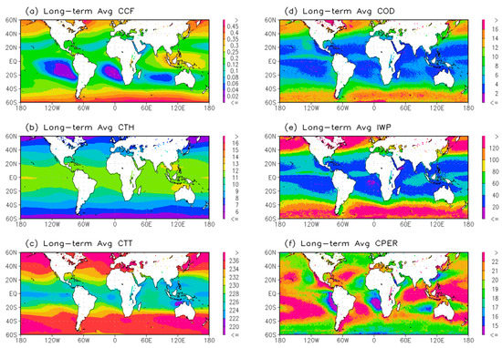
Figure 1.
Global distributions of (a) cloud cover fraction (CCF), (b) cloud top height (CTH) (km), (c) cloud top temperature (CTT) (K), (d) cloud optical depth (COD), (e) ice water path (IWP) (g/m2), and (f) cloud particle effective radius (CPER) ( µm) for their long-term averaged monthly mean values from 1981.1 to 2011.12 for cirrus clouds.
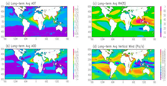
Figure 2.
Long-term mean of (a) satellite aerosol optical thickness (AOT) at 0.63 µm; (b) model aerosol optical depth (AOD) at 0.5 µm; (c) climate forecast system reanalysis relative humidity (CFSR RH) (%) averaged for six pressure levels (100 mb, 150 mb, 200 mb, 250 mb, 300 mb, and 400 mb); and (d) CFSR vertical velocity (Pa/s) on a 300 mb pressure level (negative/positive value indicate upward/downward motion).
AVHRR AOT is derived over the global ocean surface for λ1 = 0.63 µm and λ2 = 0.86 µm channels using a two-channel AVHRR aerosol retrieval algorithm [34] on AVHRR clear-sky daytime reflectance. The clear-sky reflectance data is obtained from the PATMOS-x AVHRR all-sky reflectance and cloud probability products of version 5.3 PATMOS-x AVHRR reflectance/cloud CDRs [27]. The data time period spans from 1981 to 2011, and the spatial resolution is 0.1° × 0.1° on the equal-angle grid. AOTs derived for 0.63 µm (τ1) and 0.86 µm (τ2) channels are used to calculate the aerosol Angström exponent (α) following:
The aerosol index (AIX) defined as AIX = τ1 × α, which is a better proxy for column aerosol concentration than AOT [14,35,36], will be used in our analysis. AVHRR AOT retrieval can be problematic at large solar zenith angles [37,38] beyond 60°N and 60°S latitudes (especially for winter months), resulting in poor data sampling for monthly averages of AOT and α in these regions. At the same time, cloud detection is degraded over bright snow and ice surfaces at polar latitudes. Thus, we will confine our analysis to the region between 60°S and 60°N over the global oceans. Thirty-one years (1981–2011) of monthly mean products of AVHRR aerosol and PATMOS-x AVHRR cloud CDRs are averaged to obtain long-term mean values for use in this study.
2.2. Reanalysis Data
Data for some meteorological fields that are relevant to the formation and development of aerosols and clouds are obtained from the National Centers for Environmental Prediction (NCEP) climate forecast system reanalysis (CFSR) monthly mean product (ftp://nomads.ncdc.noaa.gov/CFSR/HP_monthly_means/) with a latitude and longitude resolution of 0.5° × 0.5°. These include relative humidity (RH) in percentage for 6 pressure levels (100 mb, 150 mb, 200 mb, 250 mb, 300 mb, and 400 mb) and vertical velocity (ω) in Pa/s at a 300 mb pressure level. RH values for the six pressure levels are averaged for a mean value and used in our analysis. This averaged RH provides a general background moisture condition in the upper troposphere, where most cirrus clouds are located. NCEP CFSR was designed and executed as a global, high-resolution, coupled atmosphere-ocean-land surface-sea ice system to provide the best estimate of the state of these coupled domains over the 32-year period from January 1979 to March 2011 [39]. The selected meteorological fields from CFSR monthly mean products are averaged from 1981.1 to 2010.12 to obtain long-term mean values, which are further interpolated by using the cubic convolution of IDL subroutine into the same spatial resolution (0.1 × 0.1°) as the long-term averaged satellite products used in this study (see Figure 2c,d).
2.3. Aerosol Model Data
Aerosol simulation data from the GEOS-Chem-APM model [40,41] is also used to support our analysis and to confirm the AIE signatures identified in the satellite observation. The GEOS–Chem-APM model is a global 3-D model of atmospheric chemical composition and aerosols with size-resolved advanced particle microphysics (APM), driven by assimilated meteorological observations from the Goddard Earth observing system (GEOS) of the NASA Global Modeling Assimilation Office (GMAO). Aerosol optical depth (AOD) at 0.50 µm and number concentrations for five aerosol types (sulfate aerosols, dust particles, sea salt aerosols, black carbon aerosols, and organic aerosols) from 2000 to 2011 are available for our analysis. The horizontal resolution of the coupled model is 2° × 2.5°, and there are 47 vertical levels (aerosol number concentration is computed on 38 levels from surface to ~ 19 km). In GEOS-Chem, the emission of dust particles is calculated with the mineral dust entrainment and deposition (DEAD) scheme [42]. Dust particles are removed from the atmosphere through dry deposition and wet scavenging (rainout and washout), as described in Liu et al. [43]. The spatial and temporal variations of dust particles simulated by GEOS-Chem have been evaluated by a number of previous studies [44,45,46,47,48]. To compare the model output with satellite observations, the aerosol model data, similar to the reanalysis data, are interpolated to the same spatial resolution (0.1° × 0.1°) as the long-term averaged satellite products. Figure 2a,b are examples of global maps for long-term averaged aerosol optical thickness (AOT) (also called aerosol optical depth (AOD)) from both satellite measurements and model simulations. Hereafter, we use AOT for satellite data and AOD for model simulation in order to distinguish the two. The general patterns and magnitude of satellite AOT (at 0.63 µm) and model AOD (at 0.50 µm) are broadly consistent with each other, but a few regional differences are noticeable. For example, differences are prominent in the tropical areas influenced by aerosols from biomass burning and dust particles.
3. Methodology of Analysis
In this study, statistical correlation features between AIX and the key cloud variables, including CPER (or re), COD (or τc), IWP, CCF, CTH, and CTT, are examined and identified in order to detect AIE signatures for cirrus clouds over the global oceans. Sensitivity of the key cloud variables to AIX, defined as Δlog10(cloud-variable)/Δlog10(AIX), is also investigated for AIE imprints, which is actually the slope of linear regression between log10(cloud-variable) and log10(AIX). Logarithmic expressions used in the sensitivity computation based on a linear equation ensure that nonlinearity can be included. Long-term averaged monthly mean values (which have less noise than instantaneous values or short-term averaged values) of AIX, the six cloud variables, and the two meteorological fields (RH and ω) will be used in the statistical correlation analysis and sensitivity study to capture more robust AIE signatures from a climatology perspective. Aerosol model simulations are also used to confirm the AIE signatures manifested in the satellite observations.
4. AIE Sensitive Regimes
The AIX regimes where the signatures of AIE are likely to manifest in the long-term averaged global monthly mean data of AIX and the six key cloud variables, along with their dependence on meteorological conditions, are examined in the following section through the statistical analyses of their relationships.
4.1. Statistical Relationships
Figure 3 shows the statistic relationships of AIX with CPER, COD, IWP, CCF, CTH, and CTT for their long-term averaged values. Three regimes can be defined according to: (1) AIX < 0.18 (Regime I hereafter), (2) 0.18 < AIX < 0.46 (Regime II), and (3) AIX > 0.46 (Regime III). In Regime I, CPER increases with increasing AIX, but the corresponding COD and IWP have a decreasing trend. CCF decreases with AIX increase. CTH increases with increasing AIX, while CTT increases in the first half of the regime but then reverses to decrease in the second half. These variation features of cloud variables with increasing AIX in Regime I are consistent with the signatures of negative aerosol albedo and lifetime effects.
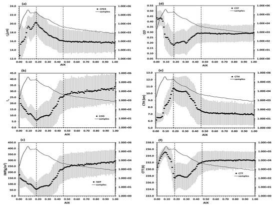
Figure 3.
Relationship (black dots) between the aerosol index (AIX) and (a) re (or CPER), (b) τc (or COD), (c) IWP, (d) CCF, (e) CTH, and (f) CTT for their long-term averaged monthly mean data over the global oceans (1981.1–2011.12). The number of data samples (black line) is measured by the vertical coordinate on the right-hand side. The data is binned according to the AIX with 0.01 incremental intervals, and the mean values for individual bins are represented by black dots. The error bars indicate one standard deviation, and the two vertical dash lines are used to divide the plot into three regimes schematically.
In Regime II, CPER decreases as AIX increases, while COD and IWP increase slowly at the beginning, followed by a rapid increase. CCF increases slowly at the beginning of Regime II, followed by a steeper increase. CTH (or CTT) decreases (or increases) slowly at the beginning, with increasing AIX followed by a steeper decrease (or increase). These variation features of cloud variables with increasing AIX in Regime II are consistent with the signatures of positive aerosol albedo and lifetime effects.
In Regime III, CPER decreases slowly with increasing AIX at the beginning and then levels off, while COD and IWP increase slowly with AIX. CCF stays nearly constant, while CTH (or CTT) decreases (or increases) slowly with increasing AIX at the beginning and then levels off. These variation features fit the signatures of neither negative nor positive aerosol albedo and lifetime effects.
More distinct trends of change for CPER, COD, CTH, and CTT in the three regimes can be seen in Figure 4, which is the scatterplot of averaged CPER versus COD and CTH versus CTT for individual AIX bins defined in Figure 3. AIX values are color-coded in the data points with black and purple dots in Regime I; blue dots in Regime II; and green, yellow, and red dots in Regime III.
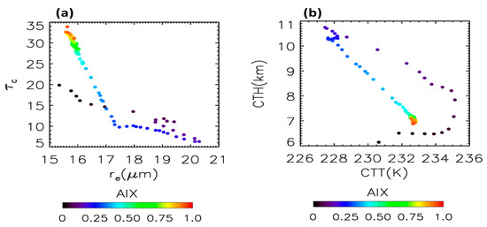
Figure 4.
Scatterplot of (a) re (or CPER) versus τc (or COD) and (b) CTT versus CTH for the mean values of CPER, COD, CTT, and CTH in individual bins of the AIX defined in Figure 3. The corresponding AIX values are color-coded for each data point.
Now, let us examine the meteorological conditions in the upper troposphere for the three AIX regimes identified above. Figure 5 shows the relationship of the AIX with RH (relative humidity averaged for the six pressure levels) and ω (vertical velocity on a 300 mb pressure level). RH decreases first, with the AIX increasing in Regime I, and reverses to increase after it falls to minimum in the middle of the regime. Upward motion (negative ω) is dominant in the first half of Regime I, which turns to subsiding motion (positive ω) in the second half of Regime I. These features suggest that most of the clouds are probably at the developing stage in the first half of Regime I, which is followed by a dissipating stage in the second half. In the developing stage, air moisture is condensed and reduced, while in the dissipating stage, air moisture is released and increased. Upward motion is dominant in Regime II, along with high RH, which suggests clouds are developing to maturity and more activated aerosols participate in the competition for water vapor so that their growing to larger cloud particles is suppressed and RH is maintained at a high value without precipitation. In Regime III, weak subsidence motion is dominant along with low RH, which suggests most of the clouds are at a dissipating stage in a dry environment. These features will be further elaborated hereafter to identify the mechanisms for aerosol-cloud interactions.
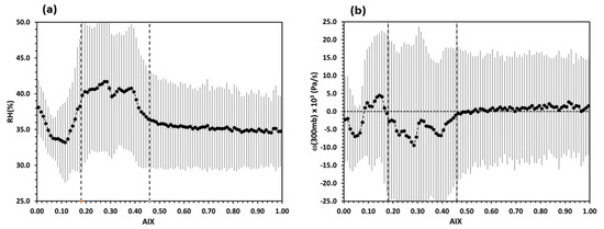
Figure 5.
Relationship of the AIX with meteorological variables (a) RH (%) and (b) ω (Pa/s) for their long-term averaged monthly mean values over the global oceans. R is the relative humidity averaged for six pressure levels (100 mb, 150 mb, 200 mb, 250 mb, 300 mb, and 400 mb). ω is vertical velocity on the 300 mb pressure level, multiplied by 103 for presentation purposes. Similar to Figure 3, the data is binned according to the AIX with 0.01 incremental intervals, the dots represent the mean value of individual AIX bins, and the error bars indicate one standard deviation. The two vertical dash lines are used to divide the plot into three regimes schematically, and the horizontal dot line in (b) is the zero vertical velocity line.
Since CPER and CCF are two cloud variables that are sensitive to the albedo effect [49] and lifetime effect [22], respectively, we examine their variations with respect to meteorological conditions. Global long-term averaged CPER and CCF are binned according to RH and ω, respectively, for the three AIX regimes (AIX < 0.18, 0.18 < AIX < 0.46, and AIX > 0.46), and their mean values for the individual bins are displayed in Figure 6. It is seen in Figure 6a that the signature of the positive aerosol albedo effect (smaller CPER corresponding to larger AIX) is likely to manifest in moist conditions (RH > 50%). Other satellite observation-based studies (e.g., [17]) found that the negative aerosol albedo effect is likely to manifest in dry conditions. Figure 6a shows that there may be a signature of negative aerosol albedo effects manifested in the AIX and RH relationship for the dry conditions (RH < 27%) between Regime II and III but not Regime I. Thus, we are cautious in drawing conclusions regarding the negative aerosol albedo effect for the dry conditions from the current statistical analysis based on long-term averaged satellite observations. The signature of the positive aerosol albedo effect is more likely to manifest in the regime of upward motion than in the regime of subsidence motion (see Figure 6b). The signature of the positive aerosol lifetime effect (larger CCF corresponding to higher AIX) is likely to manifest only in either very dry or very wet conditions (see Figure 6c) and in the regime with relatively strong upward motion (see Figure 6d). The signature of the aerosol lifetime effect manifested in the CCF variation for different AIX values is generally not as distinct and coherent as the signature of the aerosol albedo effect manifested in the CPER variation, which suggests that the cirrus cloud microphysical variable CPER is more susceptible to aerosol-cloud interaction than the macrophysical variable CCF.
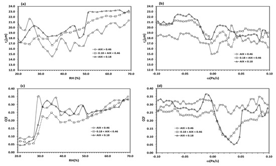
Figure 6.
Relationship of re (or CPER) with meteorological variables (a) RH (%) and (b) ω((Pa/s) and CCF with (c) RH and (d) ω for three aerosol-loading conditions: AIX < 0.18, 0.18 < AIX < 0.46, and AIX > 0.46, which correspond to the three AIX regimes defined in Figure 3. The data is binned according to RH and ω with incremental intervals of 2 and 0.005, respectively. The symbols represent the mean value of individual bins.
4.2. Physical Interpretations
When aerosol loading is very low in Regime I (pristine marine air), a low CTH value and high CTT and CCF values (see Figure 3d–f) suggest Regime I corresponds mainly to active storm zones of middle and high latitudes. The concurrent increase of CTT and CTH in the first part of this regime suggests the clouds are in elevated inversion layers, which are often observed in synoptic warm/cold front systems at middle and high latitudes. In these active storm zones, the upward motion of synoptic weather systems can maintain sufficient supersaturation and cold temperatures for heterogeneous freezing in the upper troposphere. The AIX increase in Regime I is still not sufficient to trigger the suppression of ice particle growth, which means that ice particles can grow bigger (see large CPER in Figure 3a and Figure 4a) and precipitate out because there are fewer particles competing for water vapor, which also reduces moisture accordingly (see low RH in Figure 5a). This results in a negative aerosol albedo effect, as indicated by increasing CPER together with decreasing COD and IWP when the AIX increases, as well as the negative aerosol cloud lifetime effect (decreasing CCF with increasing AIX). The cloud reduction noted in this regime most likely is caused by two processes: (1) the radiative evaporation at cloud-top during the cloud development stage (suggested by upward motion in Figure 5b) in the first half-part of Regime I. Similar cloud dissipation due to radiative evaporation was also observed by Koren et al. [50] and Altaratz et al. [51] for warm convective clouds. (2) The precipitation dissipation of larger ice particles (CPER can reach above 20 µm, as shown in Figure 4a) in the second half-part of Regime I, where subsidence motion becomes dominant (as indicated by the positive ω in Figure 5b) and CCF decreases to minimum (see Figure 3d).
In Regime II, signatures of positive aerosol albedo and lifetime effects are distinct, because CPER decreases with increasing AIX, while COD, IWP, and CCF gradually increases at the beginning, followed by a rapid increase thereafter. This signature of positive aerosol albedo or lifetime effects is very similar to that identified for warm water clouds [26]. More activated aerosols in the liquid phase participate in the competition for water vapor so that their growing to larger cloud droplets is suppressed and RH can be maintained at a high value (see Figure 5a) without precipitation. A large number of small droplets are uplifted by upward motion (see Figure 5b) to higher altitudes (see high CTH in Figure 3e and Figure 4b) in very cold temperatures (see Figure 3f and Figure 4b) to trigger glaciation. High RH and a relatively strong upward motion in this regime, as shown in Figure 5, also meet the favorable conditions of aerosol positive albedo and lifetime effects for ice clouds identified in Figure 6.
As we noted above, the variation features of six cloud variables relative to increasing AIX in Regime III fit neither the characteristics of negative aerosol albedo and lifetime effects nor those of positive aerosol albedo and lifetime effects. Further examinations are performed next to allow proper interpretations of the variation features of the cloud variables in Regime III.
4.3. Further Deliberation
Cirrus clouds are formed primarily from two ice-forming mechanisms [52]: the freezing of uplifted liquid droplets and IN deposition freezing [1,53]. Moreover, dust particles with global distribution due to transport are the major contributor to both CCN [54,55,56] and IN [54,57,58] in the troposphere. Thus, as a first order of approximation, the total column number concentration of dust particles is considered as a proxy for IN abundance for our current study based on long-term averaged monthly mean values. Accordingly, the relationship of AIX and AOT with the total column number concentration of dust particles (expressed as TC_Dust hereafter) from the aerosol model simulation is also examined in our study. Figure 7 shows the statistical relationship between model-based TC_Dust and satellite-based AIX and AOT for their global long-term averaged values from 2000 to 2011 (the overlapping time period between the available model simulations and the satellite observations). The global long-term averaged AIX and AOT in 0.1° × 0.1° grid boxes are binned according to the corresponding TC_Dust. The mean values of AIX and AOT and the sample numbers for each bin are plotted.
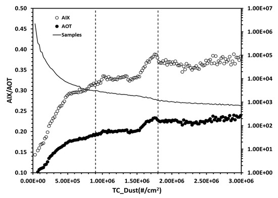
Figure 7.
Long-term averaged global ocean AIX and AOT binned according to the corresponding total column number concentration of dust particles (TC_Dust) with 2.0 × 10⁴ incremental intervals. The mean values of AIX and AOT for individual bins are displayed using the two symbols, respectively. The general line is the sample number for each bin, and the corresponding values are given by the vertical coordinate on the right-hand side. Two vertical dash lines divide the plot into three regimes schematically.
In general, AIX and AOT increase with the increase of TC_Dust; therefore, they can be used as a proxy for the abundance of dust particles. As AIX increases at a much faster rate than AOT, it should be considered a better proxy for the abundance of dust particles. Three regimes for TC_Dust, roughly divided by two vertical dash lines in Figure 7, can be defined based on how fast AIX increases with the increasing TC_Dust. AIX increase is much steeper in the first regime, defined by TC_Dust < 9.0 ×10⁴ (#/cm2) (named Regime 1 hereafter). Growth of the AIX in this regime is the fastest among the three regimes; therefore, using the AIX as a proxy for IN or CCN abundance should be effective in Regime 1. AIX increases generally with the increasing TC_Dust in Regime 2 (9.0 ×10⁴ (#/cm2) < TC_Dust < 1.8 ×10⁶ (#/cm2)), even though the growth is not as fast and smooth as in Regime 1. Thus, AIX still can be used as a proxy for IN or CCN abundance, but its efficacy as a proxy for IN or CCN abundance in this regime is not as optimal as in Regime 1. In Regime 3 (TC_Dust > 1.8 ×10⁶ (#/cm2)), the dependence of AIX on TC_Dust is the weakest among the three regimes. Thus, caution is necessary when using AIX as a proxy for IN or CCN abundance in Regime 3 in the interpretation of the results.
It is also worthwhile to examine the relationships of model-based TC_Dust with the cloud variables to see if they are consistent with the relationships between satellite-based AIX and the same cloud variables determined above. Figure 8 shows the statistic relationships of TC_Dust with CPER, COD, IWP, CCF, CTH, and CTT for their long-term averaged values. The same three regimes as defined in Figure 7 are also noted.
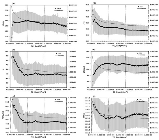
Figure 8.
Similar to Figure 3, but for the relationships between TC_Dust and (a) re (or CPER), (b) τc (or COD), (c) IWP, (d) CCF, (e) CTH, and (f) CTT for their long-term averaged monthly mean data over the global oceans (2000.1–2011.12).
In Regime 1, CPER increases with increasing TC_Dust, but the corresponding COD, IWP, and CCF have a decreasing trend. CTH increases with increasing TC_Dust, while CTT increases in the first half-part of the regime and reverses to decrease in the second-half part. The variation trends of these six cloud variables relative to the increase of TC_Dust are consistent with their variation trends due to the increase of AIX in the corresponding Regime I.
In Regime 2, the decreasing trend of CPER with increasing TC_Dust is consistent with its decreasing trend with the AIX increase in Regime II. The change tendency of COD and IWP with increasing TC_Dust in the first-half part of Regime 2 is marginally consistent with their change tendency due to increasing the AIX in Regime II. However, in the second-half part of Regime 2, their changing trend with TC_Dust is different from that due to the AIX increase. CCF shows a minor decreasing trend with increasing TC_Dust that is different from its changing trend with the AIX increase in Regime II. CTH (or CTT) shows a minor decrease (or increase) trend with the increase of TC_Dust in the first-half part of Regime 2 but reverses to marginally increase (or decrease) in the second-half part of the regime, which is consistent with their variation trends in the first-half part of Regime II but very different from those in the second-half part of Regime II. These results also corroborate the conclusion drawn in the above discussion of Figure 7 that the efficacy of the AIX serving as a proxy for IN or CCN abundance in Regime II is not as optimal as in Regime I.
In Regime 3, CPER, COD, and IWP have a minor increasing tendency at the beginning but then turn to decrease slowly with increasing TC_Dust, which is inconsistent with their changing trends in Regime III. CCF decreases slowly in Regime III but stays nearly constant in Regime III. CTH (or CTT) decreases (or increases) slowly with increasing TC_Dust at the beginning, followed by a marginal increase (or decrease). Correspondingly, CTH (or CTT) decreases (or increases) slowly with the increasing AIX at the beginning and then levels off in Regime III.
The variation trends of six cloud variables with the increasing AIX in Regime III (unlike Regimes I and II) are not consistent with their corresponding variation trends with the increase of TC_Dust in Regime 3. There are also fewer statistical sample numbers of observations in this regime in comparison to the other two regimes. As a result, there is a lack of confidence in the features revealed in the statistical relationship of our satellite observations based on the assumption of the AIX as the proxy for IN or CCN abundance in this regime. Moreover, the weak changing trends of six cloud variables with increasing total column number concentrations of dust particles do not match with the signature of positive or negative aerosol albedo effects (or lifetime effects). These factors suggest that the aerosol effect on cirrus clouds revealed in Regime III in the above statistical relationship is weak and ambiguous, and cloud macrophysical processes probably obscure or interrupt the signature of the aerosol indirect effect.
5. AIE Active Regions
To determine the active regions of the aerosol-cloud interaction in cirrus clouds over the global oceans, the sensitivity of cloud variables relative to the AIX defined as Δlog10(cloud-varibale)/Δlog10(AIX) is investigated. This sensitivity is actually the slope of the linear regression of a cloud variable relative to the AIX [59]. Thus, we performed linear regression calculations for log10(cloud-variable) relative to log10(AIX) on a 2.5° × 2.5° spatial grid over the global oceans using their long-term averaged monthly mean values in 0.1° × 0.1° spatial resolution. Using the logarithm considers the nonlinearity aspect of the sensitivity computation based on the linear regression, and the results can be used effectively to diagnose and capture the signatures of aerosol-cloud interactions [59,60].
5.1. Active Regions of Aerosol Albedo Effect
Global distributions of CPER, COD, IWP, and CCF sensitivity to the AIX variations are shown in Figure 9. A negative sensitivity of CPER and a positive sensitivity of COD and IWP to the AIX variation over the southeast coastal ocean of China in a swath region extending from 10°N to 30°N manifest a signature of positive aerosol albedo effects. A similar signature of positive aerosol albedo effects manifests in a swath region extending from 20°N to 30°N over the southeast coastal ocean of the USA and the high latitudes of the North Pacific Ocean. The confidence level of the sensitivity over these regions are generally above 95%, as shown by the contours in Figure 9. The signature of a positive aerosol albedo effect is also noticed over a broad region from 40°S to 60°S of the Southern Ocean, but the confidence level is generally below 95%. The negative sensitivity (with a confidence level above 95%) of COD to CPER variation shown in Figure 10a further corroborates that a positive aerosol albedo effect is active in these four oceanic regions. The relationship revealed by the sensitivity analysis suggests that the conventional aerosol albedo effect for cirrus clouds is easy to manifest in these four oceanic regions.
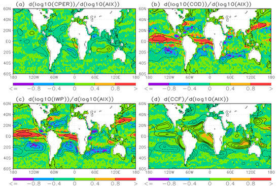
Figure 9.
Global distributions for the sensitivity to the AIX variation of (a) CPER, (b) COD, (c) IWP, and (d) CCF. The areas where the confidence level of the sensitivity is above 95% are marked by the contours. The calculation is performed for 2.5° × 2.5° spatial grids over the global oceans using the long-term averaged monthly mean values in 0.1° × 0.1° spatial resolution.
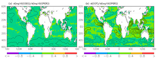
Figure 10.
Similar to Figure 9 but for the sensitivity of (a) COD and (b) CCF to CPER variation. The areas where the confidence level of the sensitivity is above 95% are marked by the contours.
Other regions with evident a negative sensitivity of CPER to the AIX variation are mainly observed in tropical and subtropical regions, such as the negative contouring areas over the tropical Atlantic Oceans, subtropical North and South Atlantic Oceans, Arabian Sea, subtropical Southwest and Northwest Pacific Oceans, and the west coast of Columbia/Ecuador. The corresponding sensitivity of COD and IWP to the AIX variations in these regions is also negative in general. This suggests that the signature of a positive aerosol albedo effect manifests only in CPER in these regions but is obscured probably by cloud dynamic and thermodynamic processes for other cloud variables. Stronger upward or subsidence motions over these tropical or subtropical regions, as revealed in Figure 2d, supports this speculation. Thus, similar to warm water clouds, the cloud particle size of cirrus clouds is also more susceptible to the aerosol-cloud interaction than other cloud variables, which are relatively more susceptible to cloud dynamic and thermodynamic processes.
5.2. Active Regions of Aerosol Lifetime Effect
Positive sensitivity observed for CCF relative to the AIX variation (see Figure 9d) for the two swath regions with evident signatures of positive aerosol albedo effects over the southeast coastal ocean of China and the USA is a signature of the positive aerosol lifetime effect. Thus, the positive aerosol albedo effect evolves into the positive aerosol lifetime effect in these two swath regions. Over the high latitudes of the North Pacific Ocean with a signature of the positive aerosol albedo effect, the sensitivity of CCF to the AIX variation is still positive but below the 95% confidence level, which suggests a positive aerosol lifetime effect is not active even though the positive aerosol albedo effect is still marginally active. A similar conclusion can also be drawn for the southern oceans ranging from 40°S to 60°S.
For other tropical and subtropical regions with a positive aerosol albedo effect manifested only in CPER, a negative sensitivity of CCF to the AIX variation is also noticed in Figure 9d, like the negative sensitivity of COD (or IWP) to the AIX variation observed in the same regions (see Figure 9b,c). Moreover, the sensitivity of CCF to CPER variation in these tropical and subtropical oceanic regions are generally positive and above a 95% confidence level, as shown in Figure 10b. These features suggest that the signature of the positive aerosol lifetime effect is probably corrupted by cloud dynamic and thermodynamic processes or smeared by the uncertainties of satellite observations. As a result, the positive aerosol albedo and lifetime effects are concealed for COD, IWP, and CCF due to their covariations with meteorological conditions determined by cloud dynamic and thermodynamic processes or the artifacts in the satellite observation. To further confirm this speculation, the sensitivity of CCF to the AIX variation is decomposed into two terms in the following equation:
Since CPER is more susceptible to the AIX variation than CCF, the first term on the right-hand side of Equation (2) contains the CCF change mainly due to CPER variation as a result of cloud-aerosol interactions. The residual term contains the CCF change mainly due to other effects, such as meteorological covariations, detection errors, etc. The term on the left-hand side and the first term on the right-hand side (along with its two components) are shown in Figure 11 for long-term averaged CCF, CPER, and AIX. Both negative and positive sensitivities clearly seen in the tropical and subtropical regions of Figure 11b (left-hand term) drop significantly in Figure 11d (first term on the right-hand side), even though the distribution patterns are similar. This confirms that the sensitivities observed in the tropical and subtropical regions of Figure 11b are mainly due to other effects (e.g., meteorological covariations) rather than to cloud-aerosol interactions, as we speculated.
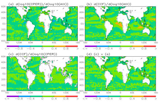
Figure 11.
Global distributions for the sensitivity of (a) CPER and (b) CCF relative to the AIX and (c) CCF relative to CPER (d) is the product of (a) and (c). The computation is performed for 2.5° × 2.5° spatial grids over the global oceans using the original long-term averaged CCF, CPER, and AIX data in 0.1° × 0.1° spatial resolution.
6. Discussions
Considering that the climate of the atmosphere represents the mean state of the atmosphere for a given time period, it is important to detect AIE signatures in long-term averaged observations. This is our major motivation for performing the current AIE study of cirrus clouds in view of the long-term mean values of aerosol and cloud variables from satellite observations. Monthly mean values of aerosol and cloud variables from satellite observations have fewer spatial gaps over the globe and with less noise comparing to their instantaneous or short-term averaged counterparts. Thus, they are more useful for identifying the sensitive regimes of aerosol-loading and active geolocations of AIE for cirrus clouds over the global oceans from a climatology perspective. Even though our statistical correlation analysis on long-term averaged aerosol and cloud variables from satellite observations is useful for detecting some signatures of AIE for cirrus clouds over the global oceans, it is important to address some possible limitations of our results.
Although AOT and AIX are often used as a proxy for CCN in passive satellite-based studies of AIE, using AOT and AIX as a proxy for IN should be done with caution, because our understanding of the chemical and physical properties of IN and its transport in the atmosphere is even more limited than for CCN. Based on both model and observational studies in the literature, we know dust particles are a major IN source in the atmosphere. Thus, without other information, we assume that using the total column number concentration of dust particles (TC_dust) as an IN proxy should be more reliable than using AOT and AIX as an IN proxy. Therefore, we added TC_dust in the statistical correlation analysis in addition to AIX, even though TC_dust is still not a perfect proxy for IN. The consistency between the results of the AIX-based analysis and TC_dust-based analysis may increase our confidence in the results. However, specific studies need to be designed in future work to quantify the uncertainties in this assumption.
Ice clouds can be formed in two major thermodynamic pathways, homogeneous and heterogeneous freezing. Homogeneous nucleation and freezing happen mainly in the upper troposphere and lower stratosphere where the temperature is very low (< -38°C) [58] and relative humidity is strongly supersaturated with respect to ice (ice supersaturation > 145%) [54,58,61,62,63,64]. Heterogeneous nucleation and freezing may happen at relatively low altitudes in the troposphere where the temperature is just below the freezing point (< 0°C) and supersaturation with respect to ice is just above 100% [54,65,66,67,68]. Depositional freezing of water vapor onto a particle surface, immersion freezing from within an aqueous coating particle, and contact freezing due to IN touch with a supercooled aqueous particle are three major pathways for heterogeneous freezing in the atmosphere [54,69,70,71]. These various freezing pathways result in very different ice cloud properties [52,72]. The formed ice clouds are generally divided into two types in observational studies [17,52,73,74] based on their distinct formation mechanisms. The first type, generated from deep convection, are named convection-generated ice clouds (including cirrus clouds due to detrainment at the cloud top). The second type, generated in situ due to the uplift motion associated with weather frontal systems, gravity waves, or orographic waves, are named in situ cirrus clouds. It is hard to effectively distinguish these two types of cirrus clouds in our statistical correlation analysis. Thus, the results obtained in this study are mainly for all types of cirrus clouds; some differentiation can be achieved based on the geolocation and altitudes of primary cirrus clouds in our above analyses but primarily in a qualitative sense.
There are also artifacts or uncertainties in the satellite observations of aerosols and ice clouds (uncertainties caused by the assumptions of aerosol optical properties, scattering properties of ice crystals, vertical distribution of ice crystals in clouds, etc.). These uncertainties may result in inconsistent features in our statistical correlation analysis for aerosol and cloud variables, such as the incoherent changing trends among cloud variables with the AIX increasing in Regime III. Thus, identifying coherent information features is critical in the detection of an AIE signature in our statistical correlation analysis. The observational uncertainties may also smear the sensitivity of cloud variables relative to the AIX variation in the detection of AIE-active regions based on our linear regression analysis. Thus, the significance of sensitivity in our regression analysis, along with the coherent correlation features between aerosol and cloud variables in the spatial distributions, are critical for identifying the signature of AIE. Therefore, our identification of the sensitive AIX regimes and active geolocations of AIE for cirrus clouds is more of a qualitative analysis. Further quantitative analyses of various processes involved in the AIE for different types of ice clouds and aerosols and their global climate implications are needed in future studies based on multiple observations (satellite, airborne, and in situ) and model (box, regional, and global) simulations.
7. Summary and Conclusions
In this study, long-term satellite AVHRR CDRs of clouds and aerosols are used to investigate the aerosol-cloud interaction of cirrus ice clouds over the global oceans for the first time from the perspective of climatology. The study focuses on determining the AIX regimes where AIE is sensitive and the geographic regions where AIE is active in the sense of a long-term average over the global oceans. Aerosol model simulation and reanalysis of meteorological fields have also been used to support our analyses.
Three AIX sensitive regimes have been identified based on the statistical relationship of satellite-observed cloud variables to the AIX variations. In the first regime (AIX < 0.18; clean marine air), CPER increases with the AIX increase while COD, IWP, and CCF decrease with the AIX increase. These features imply a signature of negative aerosol albedo and lifetime effects. The AIX can be considered as an effective proxy for IN or CCN abundance in the atmosphere in this regime. Thus, this regime is sensitive for negative aerosol albedo and lifetime effects. Relative humidity (RH) first decreases along with upward motion in this regime and then reverses to increase along with downward motion after RH falls to the minimum in the middle of the regime. In the second regime (0.18 < AIX < 0.46; moderate aerosol loading), while CPER decreases, COD, IWP, and CCF generally increase with the AIX increase. These features imply a signature of positive aerosol albedo and lifetime effects. The AIX can also be considered as a reasonable proxy for IN or CCN abundances in this regime. Therefore, this regime is sensitive for positive aerosol albedo and lifetime effects. High RH and relatively strong upward motions are the favorable meteorological conditions of the aerosol positive albedo and lifetime effects for the cirrus clouds in this regime. In the third regime (AIX > 0.46; polluted air), CPER decreases slowly with the AIX increase and then levels off, while COD, IWP, and CCF increase slowly with the AIX increase and then level off. A global aerosol model simulation provides a signature consistent with satellite observations for the first and second regimes but inconsistent for the third regime. Different features in the satellite observations and model simulation for the third regime are due to the fact that the AIX is not a reasonable proxy for IN or CCN abundance in this regime with the highest AIX. The meteorological covariations and observational artifacts probably also become the major determination factors in this regime, obscuring aerosol-cloud interaction signatures in the long-term averaged satellite observations.
Two swath regions over the southeast coastal ocean of China and the USA, the high latitude region in the North Pacific Ocean, and middle and the high latitudes of the SH oceans have been identified as the active regions for positive aerosol albedo effects. A positive aerosol lifetime effect is only active and easy to manifest in the regions with active positive aerosol albedo effects, such as the two swath regions over the southeast coastal oceans of China and the USA. Positive or negative aerosol albedos and lifetime effects in the tropics and subtropical regions are easily obscured by meteorological covariations due to relatively strong atmospheric motions and become undetectable in long-term averaged satellite observations. The results of this study based on long-term averaged satellite observations are valuable for the evaluation and improvement of the aerosol-cloud interaction in global climate models, since there are large AIE uncertainties for cirrus clouds in these models.
Author Contributions
Conceptualization, X.Z., and Y.L.; methodology and computation, X.Z.; formal analysis and investigation, X.Z., Y.L., and F.Y.; data curation, X.Z., A.K.H., and F.Y.; writing—original draft preparation, X.Z.; writing—review and editing, X.Z., Y.L., F.Y., A.K.H., and K.S. All authors have read and agreed to the published version of the manuscript.
Funding
This research was funded by the base funding of the Center for Coasts, Oceans, and Geophysics (CCOG) of NCEI (X. Zhao), the Department of Energy’s Atmospheric System Research (ASR) program (Y. Liu), NASA grant NNX17AG35G (F. Yu), funding provided by the CDR program at NCEI (A. Heidinger), and NCEI funding through a contract with the Cooperative Institute for Satellite Earth System Studies (CISESS)—Maryland at the University of Maryland in College Park (K. Saha).
Acknowledgments
The authors (X. Zhao, and A. Heidinger) would like to acknowledge support from the CDR program at the National Centers for Environmental Information (NCEI) of NOAA/NESDIS. Y. Liu is supported by the Department of Energy’s Atmospheric System Research (ASR) program, F. Yu is supported by NASA under grant NNX17AG35G, and K. Saha is supported by NCEI through a contract with the Cooperative Institute for Satellite Earth System Studies (CISESS)—Maryland at the University of Maryland in College Park. Three reviewers’ comments and suggestions helped us improve the paper immensely. Proofreading of the paper by English editor Mark Essig in NCEI is greatly appreciated. The views, opinions, and findings contained in this paper are those of the author(s) and should not be construed as an official National Oceanic and Atmospheric Administration or U.S. Government position, policy, or decision.
Conflicts of Interest
The authors declare no conflict of interest.
Acronyms
| AIE | aerosol indirect effect |
| AIX | aerosol index |
| AOD | aerosol optical depth |
| AOT | aerosol optical thickness |
| APM | aerosol particle microphysics |
| AVHRR | Advanced Very High-Resolution Radiometer |
| CCF | cloud cover fraction |
| CCN | cloud condensation nuclei |
| CDR(s) | climate data record(s) |
| CFSR | climate forecast system reanalysis |
| COD | cloud optical depth |
| CPER | cloud particle effective radius |
| CTH | cloud top height |
| CTT | cloud top temperature |
| DEAD | mineral dust entrainment and deposition |
| GAC | global area coverage |
| GEOS | Goddard Earth Observing System |
| GMAO | Global Modeling Assimilation Office |
| IN | ice nuclei |
| IWP | ice water path |
| NASA | National Aeronautics and Space Administration |
| MODIS | Moderate-resolution Imaging Spectroradiometer |
| NCEI | National Centers for Environmental Information |
| NCEP | National Centers for Environmental Prediction |
| NESDIS | National Environmental Satellite, Data, and Information Service |
| NOAA | National Oceanic and Atmospheric Administration |
| PATMOS-x | Pathfinder Atmospheres-Extended |
| RH | relative humidity |
| SH | south hemisphere |
| STAR | Center for Satellite Applications and Research |
References
- Cziczo, D.J.; Froyd, K.D.; Hoose, C.; Jensen, E.J.; Diao, M.H.; Zondlo, M.A.; Smith, J.B.; Twohy, C.H.; Murphy, D.M. Clarifying the dominant sources and mechanisms of cirrus cloud formation. Science 2013, 340, 1320–1324. [Google Scholar] [CrossRef]
- Lohmann, U. Possible aerosol effects on ice clouds via contact nucleation. J. Atmos. Sci. 2002, 59, 647–656. [Google Scholar] [CrossRef]
- Lohmann, U.; Feichter, J. Global indirect aerosol effects: A review. Atmos. Chem. Phys. 2005, 5, 715–737. [Google Scholar] [CrossRef]
- Sassen, K.; Khvorostyanov, V.I. Cloud effects from boreal forest fire smoke: Evidence for ice nucleation from polarization lidar data and cloud model simulations. Environ. Res. Lett. 2008, 3. [Google Scholar] [CrossRef]
- Penner, J.E.; Chen, Y.; Wang, M.; Liu, X. Possible influence of anthropogenic aerosols on cirrus clouds and anthropogenic forcing. Atmos. Chem. Phys. 2009, 9, 879–896. [Google Scholar] [CrossRef]
- Rosenfeld, D. Suppression of rain and snow by urban and industrial air pollution. Science 2000, 287, 1793–1796. [Google Scholar] [CrossRef]
- Li, Z.Q.; Rosenfeld, D.; Fan, J.W. Aerosols and their impact on radiation, clouds, precipitation, and severe weather events. In Oxford Research Encyclopedia of Environmental Science; Oxford University Press: New York, NY, USA, 2017; pp. 1–36. [Google Scholar]
- Ramanathan, V.; Crutzen, P.J.; Kiehl, J.T.; Rosenfeld, D. Atmosphere - aerosols, climate, and the hydrological cycle. Science 2001, 294, 2119–2124. [Google Scholar] [CrossRef]
- Rosenfeld, D.; Lohmann, U.; Raga, G.B.; O’Dowd, C.D.; Kulmala, M.; Fuzzi, S.; Reissell, A.; Andreae, M.O. Flood or drought: How do aerosols affect precipitation? Science 2008, 321, 1309–1313. [Google Scholar] [CrossRef]
- Seinfeld, J.H.; Bretherton, C.; Carslaw, K.S.; Coe, H.; DeMott, P.J.; Dunlea, E.J.; Feingold, G.; Ghan, S.; Guenther, A.B.; Kahn, R.; et al. Improving our fundamental understanding of the role of aerosol-cloud interactions in the climate system. P. Natl. Acad. Sci. USA 2016, 113, 5781–5790. [Google Scholar] [CrossRef]
- Coakley, J.A.; Bernstein, R.L.; Durkee, P.A. Effect of ship-stack effluents on cloud reflectivity. Science 1987, 237, 1020–1022. [Google Scholar] [CrossRef]
- Breon, F.M.; Tanre, D.; Generoso, S. Aerosol effect on cloud droplet size monitored from satellite. Science 2002, 295, 834–838. [Google Scholar] [CrossRef] [PubMed]
- Rosenfeld, D.; Woodley, W. Pollution and clouds. Phys. World 2001, 14, 33–37. [Google Scholar] [CrossRef]
- Nakajima, T.; Higurashi, A.; Kawamoto, K.; Penner, J.E. A possible correlation between satellite-derived cloud and aerosol microphysical parameters. Geophys. Res. Lett. 2001, 28, 1171–1174. [Google Scholar] [CrossRef]
- Huang, J.P.; Minnis, P.; Lin, B.; Wang, T.H.; Yi, Y.H.; Hu, Y.X.; Sun-Mack, S.; Ayers, K. Possible influences of asian dust aerosols on cloud properties and radiative forcing observed from modis and ceres. Geophys. Res. Lett. 2006, 33. [Google Scholar] [CrossRef]
- Jiang, J.H.; Su, H.; Zhai, C.; Massie, S.T.; Schoeberl, M.R.; Colarco, P.R.; Platnick, S.; Gu, Y.; Liou, K.N. Influence of convection and aerosol pollution on ice cloud particle effective radius. Atmos. Chem. Phys. 2011, 11, 457–463. [Google Scholar] [CrossRef]
- Zhao, B.; Liou, K.N.; Gu, Y.; Jiang, J.H.; Li, Q.B.; Fu, R.; Huang, L.; Liu, X.H.; Shi, X.J.; Su, H.; et al. Impact of aerosols on ice crystal size. Atmos. Chem. Phys. 2018, 18, 1065–1078. [Google Scholar] [CrossRef]
- Sekiguchi, M.; Nakajima, T.; Suzuki, K.; Kawamoto, K.; Higurashi, A.; Rosenfeld, D.; Sano, I.; Mukai, S. A study of the direct and indirect effects of aerosols using global satellite data sets of aerosol and cloud parameters. J. Geophys. Res-Atmos. 2003, 108. [Google Scholar] [CrossRef]
- Zhao, X.P.; Liu, Y.G.; Yu, F.Q.; Heidinger, A.K. Using long-term satellite observations to identify sensitive regimes and active regions of aerosol indirect effects for liquid clouds over global oceans. J. Geophys. Res-Atmos. 2018, 123, 457–472. [Google Scholar] [CrossRef]
- Chylek, P.; Dubey, M.K.; Lohmann, U.; Ramanathan, V.; Kaufman, Y.J.; Lesins, G.; Hudson, J.; Altmann, G.; Olsen, S. Aerosol indirect effect over the indian ocean. Geophys. Res. Lett. 2006, 33. [Google Scholar] [CrossRef]
- Twomey, S. Pollution and planetary albedo. Atmos. Environ. 1974, 8, 1251–1256. [Google Scholar] [CrossRef]
- Albrecht, B.A. Aerosols, cloud microphysics, and fractional cloudiness. Science 1989, 245, 1227–1230. [Google Scholar] [CrossRef] [PubMed]
- Givati, A.; Rosenfeld, D. Separation between cloud-seeding and air-pollution effects. J. Appl. Meteorol. 2005, 44, 1298–1314. [Google Scholar] [CrossRef]
- Jensen, E.J.; Toon, O.B. The potential impact of soot particles from aircraft exhaust on cirrus clouds. Geophys. Res. Lett. 1997, 24, 249–252. [Google Scholar] [CrossRef]
- Karcher, B.; Mohler, O.; DeMott, P.J.; Pechtl, S.; Yu, F. Insights into the role of soot aerosols in cirrus cloud formation. Atmos. Chem. Phys. 2007, 7, 4203–4227. [Google Scholar] [CrossRef]
- Zhao, X.P.; Heidinger, A.K.; Walther, A. Climatology analysis of aerosol effect on marine water cloud from long-term satellite climate data records. Remote Sens. 2016, 8, 300. [Google Scholar] [CrossRef]
- Heidinger, A.K.; Foster, M.J.; Walther, A.; Zhao, X.P. The pathfinder atmospheres-extended avhrr climate dataset. Bull. Am. Meteorolo. Soc. 2014, 95. [Google Scholar] [CrossRef]
- Walther, A.; Heidinger, A.K. Implementation of the daytime cloud optical and microphysical properties algorithm (dcomp) in patmos-x. J. Appl. Meteorol. Clim. 2012, 51, 1371–1390. [Google Scholar] [CrossRef]
- Cao, C.; Weinreb, M.; Xu, H. Predicting simultaneous nadir overpasses among polar-orbiting meteorological satellites for the intersatellite calibration of radiometers. J. Atmos. Ocean. Technol. 2004, 21, 537–542. [Google Scholar] [CrossRef]
- Cao, C.Y.; Xiong, X.X.; Wu, A.H.; Wu, X.Q. Assessing the consistency of avhrr and modis l1b reflectance for generating fundamental climate data records. J. Geophys. Res-Atmos. 2008, 113. [Google Scholar] [CrossRef]
- Heidinger, A.K.; Cao, C.; Sullivan, J.T. Using moderate resolution imaging spectrometer (MODIS) to calibrate advanced very high resolution radiometer reflectance channels. J. Geophys. Res. 2002, 107, 4702. [Google Scholar] [CrossRef]
- Heidinger, A.K.; Straka, W.C.; Molling, C.C.; Sullivan, J.T.; Wu, X.Q. Deriving an inter-sensor consistent calibration for the avhrr solar reflectance data record. Inter. J. Remote Sens. 2010, 31, 6493–6517. [Google Scholar] [CrossRef]
- Pavolonis, M.J.; Heidinger, A.K.; Uttal, T. Daytime global cloud typing from avhrr and viirs: Algorithm description, validation, and comparisons. J. Appl. Meteorol. 2005, 44, 804–826. [Google Scholar] [CrossRef]
- Zhao, X.-P.; Dubovik, O.; Smirnov, A.; Holben, B.N.; Sapper, J.; Pietras, C.; Voss, K.J.; Frouin, R. Regional evaluation of an advanced very high resolution radiometer (AVHRR) two-channel aerosol retrieval algorithm. J. Geophys. Res. 2004, 109, D02204. [Google Scholar] [CrossRef]
- Liu, J.J.; Li, Z.Q. Estimation of cloud condensation nuclei concentration from aerosol optical quantities: Influential factors and uncertainties. Atmos. Chem. Phys. 2014, 14, 471–483. [Google Scholar] [CrossRef]
- Stier, P. Limitations of passive remote sensing to constrain global cloud condensation nuclei. Atmos. Chem. Phys. 2016, 16, 6595–6607. [Google Scholar] [CrossRef]
- Ignatov, A.; Stowe, L. Aerosol retrievals from individual avhrr channels. Part ii: Quality control, probability distribution functions, information content, and consistency checks of retrievals. J. Atmos. Sci. 2002, 59, 335–362. [Google Scholar] [CrossRef]
- Stowe, L.L.; Ignatov, A.M.; Singh, R.R. Development, validation, and potential enhancements to the second-generation operational aerosol product at the national environmental satellite, data, and information service of the national oceanic and atmospheric administration. J. Geophys. Res-Atmos. 1997, 102, 16923–16934. [Google Scholar] [CrossRef]
- Saha, S.; Moorthi, S.; Pan, H.L.; Wu, X.R.; Wang, J.D.; Nadiga, S.; Tripp, P.; Kistler, R.; Woollen, J.; Behringer, D.; et al. The ncep climate forecast system reanalysis. Bull. Am. Meteorol. Soc. 2010, 91, 1015–1057. [Google Scholar] [CrossRef]
- Yu, F.; Luo, G. Simulation of particle size distribution with a global aerosol model: Contribution of nucleation to aerosol and ccn number concentrations. Atmos. Chem. Phys. 2009, 9, 7691–7710. [Google Scholar] [CrossRef]
- Yu, F.Q.; Nair, A.A.; Luo, G. Long-term trend of gaseous ammonia over the united states: Modeling and comparison with observations. J. Geophys. Res-Atmos. 2018, 123, 8315–8325. [Google Scholar] [CrossRef]
- Bian, H.S.; Zender, C.S. Mineral dust and global tropospheric chemistry: Relative roles of photolysis and heterogeneous uptake. J. Geophys. Res-Atmos. 2003, 108. [Google Scholar] [CrossRef]
- Liu, H.Y.; Jacob, D.J.; Bey, I.; Yantosca, R.M. Constraints from pb-210 and be-7 on wet deposition and transport in a global three-dimensional chemical tracer model driven by assimilated meteorological fields. J. Geophys. Res-Atmos. 2001, 106, 12109–12128. [Google Scholar] [CrossRef]
- Fairlie, T.D.; Jacob, D.J.; Dibb, J.E.; Alexander, B.; Avery, M.A.; van Donkelaar, A.; Zhang, L. Impact of mineral dust on nitrate, sulfate, and ozone in transpacific asian pollution plumes. Atmos. Chem. Phys. 2010, 10, 3999–4012. [Google Scholar] [CrossRef]
- Kim, P.S.; Jacob, D.J.; Fisher, J.A.; Travis, K.; Yu, K.; Zhu, L.; Yantosca, R.M.; Sulprizio, M.P.; Jimenez, J.L.; Campuzano-Jost, P.; et al. Sources, seasonality, and trends of southeast us aerosol: An integrated analysis of surface, aircraft, and satellite observations with the geos-chem chemical transport model. Atmos. Chem. Phys. 2015, 15, 10411–10433. [Google Scholar] [CrossRef]
- Ridley, D.A.; Heald, C.L.; Kok, J.F.; Zhao, C. An observationally constrained estimate of global dust aerosol optical depth. Atmos. Chem. Phys. 2016, 16, 15097–15117. [Google Scholar] [CrossRef]
- Li, S.; Zhang, L.; Cai, K.; Ge, W.; Zhang, X. Comparisons of the vertical distributions of aerosols in the calipso and geos-chem datasets in china. Atmos. Environ. X 2019, 3, 100036. [Google Scholar] [CrossRef]
- Zhang, Y.D.; Luo, G.; Yu, F.Q. Seasonal variations and long-term trend of dust particle number concentration over the northeastern united states. J. Geophys. Res-Atmos. 2019, 124, 13140–13155. [Google Scholar] [CrossRef]
- Twomey, S.A. Influence of Pollution on Shortwave Albedo of Clouds. J. Atmos. Sci. 1977, 34, 1149–1152. [Google Scholar] [CrossRef]
- Koren, I.; Dagan, G.; Altaratz, O. From aerosol-limited to invigoration of warm convective clouds. Science 2014, 344, 1143–1146. [Google Scholar] [CrossRef]
- Altaratz, O.; Koren, I.; Remer, L.A.; Hirsch, E. Review: Cloud invigoration by aerosols-coupling between microphysics and dynamics. Atmos. Res. 2014, 140, 38–60. [Google Scholar] [CrossRef]
- Kramer, M.; Rolf, C.; Luebke, A.; Afchine, A.; Spelten, N.; Costa, A.; Meyer, J.; Zoger, M.; Smith, J.; Herman, R.L.; et al. A microphysics guide to cirrus clouds - part 1: Cirrus types. Atmos. Chem. Phys. 2016, 16, 3463–3483. [Google Scholar] [CrossRef]
- Froyd, K.D.; Cziczo, D.J.; Hoose, C.; Jensen, E.J.; Diao, M.H.; Zondlo, M.A.; Smith, J.B.; Twohy, C.H.; Murphy, D.M. Cirrus cloud formation and the role of heterogeneous ice nuclei. Aip. Conf. Proc. 2013, 1527, 976–978. [Google Scholar]
- Pruppacher, H.R.; Klett, J.D. Microphysics of Clouds and Precipitation; Springer: Dordretch, The Netherlands, 1997; p. 954. [Google Scholar] [CrossRef]
- Karydis, V.A.; Kumar, P.; Barahona, D.; Sokolik, I.N.; Nenes, A. On the effect of dust particles on global cloud condensation nuclei and cloud droplet number. J. Geophys. Res-Atmos 2011, 116. [Google Scholar] [CrossRef]
- Karydis, V.A.; Tsimpidi, A.P.; Bacer, S.; Pozzer, A.; Nenes, A.; Lelieveld, J. Global impact of mineral dust on cloud droplet number concentration. Atmos. Chem. Phys. 2017, 17, 5601–5621. [Google Scholar] [CrossRef]
- Hoose, C.; Mohler, O. Heterogeneous ice nucleation on atmospheric aerosols: A review of results from laboratory experiments. Atmos. Chem. Phys. 2012, 12, 9817–9854. [Google Scholar] [CrossRef]
- Kanji, Z.A.; Ladino, L.A.; Wex, H.; Boose, Y.; Burkert-Kohn, M.; Cziczo, D.J.; Krämer, M. Overview of ice nucleating particles. Meteorol. Monogr. 2017, 58, 1.1–1.33. [Google Scholar] [CrossRef]
- Gryspeerdt, E.; Stier, P. Regime-based analysis of aerosol-cloud interactions. Geophys. Res. Lett. 2012, 39. [Google Scholar] [CrossRef]
- Gryspeerdt, E.; Stier, P.; Grandey, B.S. Cloud fraction mediates the aerosol optical depth-cloud top height relationship. Geophys. Res. Lett. 2014, 41, 3622–3627. [Google Scholar] [CrossRef]
- Koop, T.; Ng, H.P.; Molina, L.T.; Molina, M.J. A new optical technique to study aerosol phase transitions: The nucleation of ice from h2so4 aerosols. J. Phys. Chem. A 1998, 102, 8924–8931. [Google Scholar] [CrossRef]
- Mohler, O.; Bunz, H.; Stetzer, O. Homogeneous nucleation rates of nitric acid dihydrate (NAD) at simulated stratospheric conditions - part ii: Modelling. Atmos. Chem. Phys. 2006, 6, 3035–3047. [Google Scholar] [CrossRef]
- Richardson, M.S.; DeMott, P.J.; Kreidenweis, S.M.; Petters, M.D.; Carrico, C.M. Observations of ice nucleation by ambient aerosol in the homogeneous freezing regime. Geophys. Res. Lett. 2010, 37. [Google Scholar] [CrossRef]
- Stetzer, O.; Mohler, O.; Wagner, R.; Benz, S.; Saathoff, H.; Bunz, H.; Indris, O. Homogeneous nucleation rates of nitric acid dihydrate (nad) at simulated stratospheric conditions - part i: Experimental results. Atmos. Chem. Phys. 2006, 6, 3023–3033. [Google Scholar] [CrossRef]
- DeMott, P.J.; Sassen, K.; Poellot, M.R.; Baumgardner, D.; Rogers, D.C.; Brooks, S.D.; Prenni, A.J.; Kreidenweis, S.M. African dust aerosols as atmospheric ice nuclei. Geophys. Res. Lett. 2003, 30. [Google Scholar] [CrossRef]
- DeMott, P.J.; Prenni, A.J. New directions: Need for defining the numbers and sources of biological aerosols acting as ice nuclei. Atmos. Environ. 2010, 44, 1944–1945. [Google Scholar] [CrossRef]
- DeMott, P.J.; Prenni, A.J.; Liu, X.; Kreidenweis, S.M.; Petters, M.D.; Twohy, C.H.; Richardson, M.S.; Eidhammer, T.; Rogers, D.C. Predicting global atmospheric ice nuclei distributions and their impacts on climate. P. Natl. Acad. Sci. USA 2010, 107, 11217–11222. [Google Scholar] [CrossRef] [PubMed]
- Lynch, F.; Khodadoust, A. Effects of ice accretions on aircraft aerodynamics. Prog. Aerosp. Sci. 2002, 38, 273–274. [Google Scholar] [CrossRef]
- Field, P.R.; Mohler, O.; Connolly, P.; Kramer, M.; Cotton, R.; Heymsfield, A.J.; Saathoff, H.; Schnaiter, M. Some ice nucleation characteristics of asian and saharan desert dust. Atmos. Chem. Phys. 2006, 6, 2991–3006. [Google Scholar] [CrossRef]
- Mohler, O.; Buttner, S.; Linke, C.; Schnaiter, M.; Saathoff, H.; Stetzer, O.; Wagner, R.; Kramer, M.; Mangold, A.; Ebert, V.; et al. Effect of sulfuric acid coating on heterogeneous ice nucleation by soot aerosol particles. J. Geophys. Res-Atmos. 2005, 110. [Google Scholar] [CrossRef]
- Mohler, O.; Field, P.R.; Connolly, P.; Benz, S.; Saathoff, H.; Schnaiter, M.; Wagner, R.; Cotton, R.; Kramer, M.; Mangold, A.; et al. Efficiency of the deposition mode ice nucleation on mineral dust particles. Atmos. Chem. Phys. 2006, 6, 3007–3021. [Google Scholar] [CrossRef]
- Luebke, A.E.; Afchine, A.; Costa, A.; Grooss, J.U.; Meyer, J.; Rolf, C.; Spelten, N.; Avallone, L.M.; Baumgardner, D.; Kramer, M. The origin of midlatitude ice clouds and the resulting influence on their microphysical properties. Atmos. Chem. Phys. 2016, 16, 5793–5809. [Google Scholar] [CrossRef]
- Mace, G.G.; Clothiaux, E.E.; Ackerman, T.P. The composite characteristics of cirrus clouds: Bulk properties revealed by one year of continuous cloud radar data. J. Climate 2001, 14, 2185–2203. [Google Scholar] [CrossRef]
- Mace, G.G.; Benson, S.; Vernon, E. Cirrus clouds and the large-scale atmospheric state: Relationships revealed by six years of ground-based data. J. Climate 2006, 19, 3257–3278. [Google Scholar] [CrossRef]


© 2020 by the authors. Licensee MDPI, Basel, Switzerland. This article is an open access article distributed under the terms and conditions of the Creative Commons Attribution (CC BY) license (http://creativecommons.org/licenses/by/4.0/).