Article

Estimating the Growing Stem Volume of Chinese Pine and Larch Plantations based on Fused Optical Data Using an Improved Variable Screening Method and Stacking Algorithm

1
Research Center of Forestry Remote Sensing & Information Engineering, Central South University of Forestry and Technology, Changsha 410004, China
2
School of Information Science and Engineering, Hunan First Normal University, Changsha 410205, China
3
Key Laboratory of Forestry Remote Sensing Based Big Data & Ecological Security for Hunan Province, Changsha 410004, China
4
Key Laboratory of State Forestry Administration on Forest Resources Management and Monitoring in Southern Area, Changsha 410004, China
5
Department of Geography and Environmental Resources, Southern Illinois University, Carbondale, IL 62901, USA
*
Author to whom correspondence should be addressed.
Remote Sens. 2020, 12(5), 871; https://doi.org/10.3390/rs12050871
Submission received: 31 December 2019 / Revised: 11 February 2020 / Accepted: 5 March 2020 / Published: 9 March 2020

Abstract

:
Accurately estimating growing stem volume (GSV) is very important for forest resource management. The GSV estimation is affected by remote sensing images, variable selection methods, and estimation algorithms. Optical images have been widely used for modeling key attributes of forest stands, including GSV and aboveground biomass (AGB), because of their easy availability, large coverage and related mature data processing and analysis technologies. However, the low data saturation level and the difficulty of selecting feature variables from optical images often impede the improvement of estimation accuracy. In this research, two GaoFen-2 (GF-2) images, a Landsat 8 image, and fused images created by integrating GF-2 bands with the Landsat multispectral image using the Gram–Schmidt method were first used to derive various feature variables and obtain various datasets or data scenarios. A DC-FSCK approach that integrates feature variable screening and a combination optimization procedure based on the distance correlation coefficient and k-nearest neighbors (kNN) algorithm was proposed and compared with the stepwise regression analysis (SRA) and random forest (RF) for feature variable selection. The DC-FSCK considers the self-correlation and combination effect among feature variables so that the selected variables can improve the accuracy and saturation level of GSV estimation. To validate the proposed approach, six estimation algorithms were examined and compared, including Multiple Linear Regression (MLR), kNN, Support Vector Regression (SVR), RF, eXtreme Gradient Boosting (XGBoost) and Stacking. The results showed that compared with GF-2 and Landsat 8 images, overall, the fused image (Red_Landsat) of GF-2 red band with Landsat 8 multispectral image improved the GSV estimation accuracy of Chinese pine and larch plantations. The Red_Landsat image also performed better than other fused images (Pan_Landsat, Blue_Landsat, Green_Landsat and Nir_Landsat). For most of the combinations of the datasets and estimation models, the proposed variable selection method DC-FSCK led to more accurate GSV estimates compared with SRA and RF. In addition, in most of the combinations obtained by the datasets and variable selection methods, the Stacking algorithm performed better than other estimation models. More importantly, the combination of the fused image Red_Landsat with the DC-FSCK and Stacking algorithm led to the best performance of GSV estimation with the greatest adjusted coefficients of determination, 0.8127 and 0.6047, and the smallest relative root mean square errors of 17.1% and 20.7% for Chinese pine and larch, respectively. This study provided new insights on how to choose suitable optical images, variable selection methods and optimal modeling algorithms for the GSV estimation of Chinese pine and larch plantations.

Graphical Abstract

1. Introduction

Planted forests are important forest resources. They provide wood supply [1,2] and maintain the ecological balance with the ever increasing global climate change. The construction and sustainable management of planted forests have become important for carbon sequestration, biomass accumulation, and climate change responses under the framework of the Global Climate Change Convention [3,4,5]. Forest growing stem volume (GSV) is an important component of forest aboveground biomass (AGB) and a key parameter for assessing forest carbon balance at regional scales [5]. However, it is often difficult to directly obtain large-scale forest AGB. Usually, people measure the tree height and diameter at breast height (DBH), then use the overall growth equations to calculate GSV, and finally multiply the GSV by a biomass expansion factor to get AGB [6,7,8,9]. Therefore, GSV is the basic and key factor for the construction and sustainable management of plantations at regional scales [10,11,12]. Remote sensing images with easy access and wide temporal and spatial coverage characterize forest surface features and can be used to map the spatial patterns and dynamic changes of forest resources [13,14,15,16,17,18].
A lot of efforts have been made to explore different remote sensing data, different feature variable screening methods and modeling algorithms for improving forest GSV or AGB estimation [14,15,19,20,21,22,23,24,25,26]. Radar wave, especially long-wavelength radar wave, can penetrate forest canopies to capture the information of stems, branches and understory and thus characterize forest structures in vertical directions [13,20]. However, data saturation and complexity of data processing may influence the GSV estimation in the forests with complex stand structures, such as mature forests, when backscattering values are used [13,21]. Interferometry SAR (InSAR) can increase the data saturation levels [22,23], but its estimation accuracy is highly related to the target environment, such as wind speed, moisture, and temperature [24]. LiDAR data are powerful in estimating canopy structures but they are mainly airborne-based, which has less availability of large coverage than space-borne optical sensor data. Therefore, extensive application of LiDAR for forest GSV estimation is rare [25,26,27].
Despite the problem of data saturation [28], optical sensor data have been widely used for forest GSV estimation due to their various spatial, spectral, radiometric and temporal resolutions, mature processing technologies, abundant data sources and large coverage [16,17,18,28,29,30,31,32,33,34,35]. Many studies have applied data combination or fusion of different sensors to improve forest GSV or AGB estimation [28,30,36]. Usually, the multispectral bands of medium-resolution imagery (e.g., Landsat TM multi-spectral data) are fused with the panchromatic bands of high-resolution imagery [37,38,39,40] (e.g., SPOT panchromatic data). Compared with multispectral bands, panchromatic bands have higher spatial resolution but lower spectral resolution and relatively rough spectral characteristics [39]. Fusing multispectral and panchromatic images of different optical sensors can improve the spatial resolution, thereby helping visual interpretation. However, the data fusion method cannot add much new information, and thus offers less opportunity to enhance the GSV estimation [41].
Generally, high-resolution remote sensing images contain detailed spatial feature information but less spectral information [34]. For example, GaoFen-2 (GF-2) images have a sub-meter spatial resolution and can clearly reflect forest structural characteristics, but have only a few spectral bands (Band2_Blue, Band3_Green, Band4_Red and Band5_Nir) [42,43,44]. Medium-resolution remote sensing images usually have rich spectral information and extensive spatiotemporal coverage [30]. For example, Landsat 8 imagery has five multispectral bands plus two short-wave infrared (SWIR) bands, which can help vegetation observation. Furthermore, Landsat 8 imagery has global coverage and is free of charge [31]. Therefore, fusing GF-2 multispectral bands with Landsat 8 multispectral images will provide the potential to improve the GSV estimation of Chinese pine and larch plantations in northeastern China.
Selecting suitable feature variables from optical images is a key step in developing forest GSV estimation models [45]. Besides raw spectral data, many variables such as various band ratios, vegetation indices, and texture measures can be derived by band calculations and transformations [13,32], which offers the possibility of obtaining a large number of feature variables. However, this also leads to difficulty in selecting the variables that can significantly increase the GSV estimation accuracy. Principal component analysis (PCA) is often used to reduce the information redundancy, as it linearly combines original variables and transforms them into a set of new variables that are not correlated with each other [13,19]. The new variables are not bio-physically meaningful. In addition, Stepwise Regression Analysis (SRA) [28,30], Random Forest (RF) [13,19,46], the sure independence screening procedure based on Pearson correlation (PC-SIS) [47], the sure independence screening procedure based on distance correlation (DC-SIS) [48], and the fast iterative features selection method for k-nearest neighbor (kNN-FIFS) have also been widely used for variables selection in classification or regression modeling [49]. Unlike PCA, these methods keep the original variables and do not generate new variables when reducing the dimensionality of sample data. However, these methods do not consider the self-correlation of the variables or the combined effects of the variables. Due to the interaction and correlation between remote sensing variables, different variable combinations may lead to very different accuracies of GSV estimation [13]. Thus, we should develop a new variable selection method or improve the existing methods to overcome the gaps that currently exist and further investigate the optimal number and combination of feature variables to increase the estimation accuracy.
The estimation algorithms also influence the GSV estimation results [13,50,51,52]. Ensemble learning algorithms, such as RF, eXtreme Gradient Boosting (XGBoost) and Stacking, often have better performance than traditional regression algorithms such as Multiple Linear Regression (MLR) [53,54,55,56,57,58]. However, the ensemble learning algorithms are generally more sensitive to the characteristics of training samples, including sample sizes and representatives of population features, and thus require more training samples than the traditional parametric algorithms [13,19,45]. In addition, the performance of the algorithms may be site-specific [13,45].
This research aimed to develop an effective method for feature variable screening and identifying suitable optical images and modeling algorithms for improving the GSV estimation of planted forests. We first fused GF-2 multispectral bands with Landsat 8 multispectral images, which led to various datasets or data scenarios along with the original images. We then proposed a feature variable screening and combination optimization procedure based on the distance correlation coefficient and k-nearest neighbor algorithm (DC-FSCK). The proposed DC-FSCK method was compared with two widely used feature variable screening methods (SRA, RF) to select the optimal set of feature variables from the datasets. In Section S3 of the Supplementary Material, we described the SRA and RF methods in detail. Moreover, we validated the selections of the feature variables by comparing the performance of the parametric algorithm MLR and five nonparametric machine learning algorithms, including K-Nearest Neighbor (kNN), Support Vector Regression (SVR), RF, XGBoost and Stacking. The best method was used to map the GSV of Chinese pine and larch plantations in northern China. It was expected that this research could provide new insights on the GSV estimation of the coniferous plantations.

2. Materials and Methods

2.1. Study Area

The study area, Wangyedian Experimental Forest Farm, is located in the southwest of Harqin, Inner Mongolia of China (Figure 1), with a total area of approximately 500 km2. Influenced by the monsoon temperate continental climate, this region has an annual precipitation of 300~500 mm and an annual average temperature of 4.2 °C. The elevation of this region is higher in the southwest and lower in the northeast, with the range of 800 m to 1890 m. There are many middle mountains and low mountains [59,60]. The percentage forest cover was about 93% by the end of 2016, with a total stock volume of 1.527 million m3 [59]. The plantations occupied most of the forested area in this forest farm, mainly including larch (Larix principis-rupprechtii and Larixolgensis), Chinese pine (Pinus tabuliformis) and Scots pine (Pinus sylvestris) forests [48].

2.2. Framework of This Research

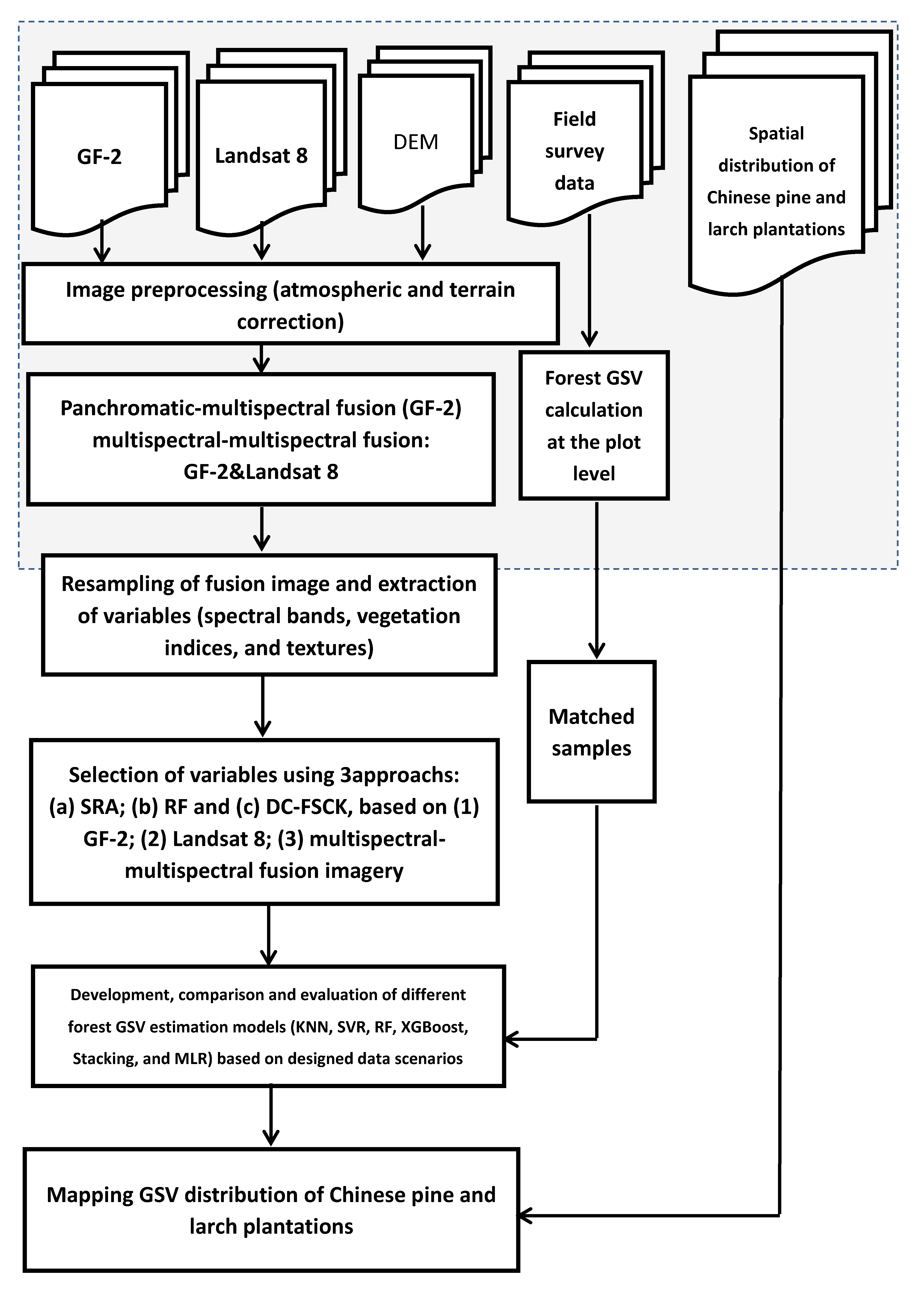
The methodological framework for mapping the GSV of Chinese pine and larch plantations using multiple datasets includes four steps: 1) Data preparation and processing; 2) Feature variable extraction; 3) Variable selection; 4) Model development, evaluation, and application (Figure 2). Based on GF-2 and Landsat 8 images, we derived various datasets, including the original and fused images, and from which we selected the best sets of feature variables, developed the relationships of GSV from the sample plots with the feature variables for Chinese pine and larch, including the spectral bands, vegetation indices and texture measures. The digital elevation model (DEM) was utilized to conduct the terrain corrections of the images. We did not calculate tree DBH and height from the remote sensing data. Therefore, the framework can be extended to other study areas if and only if there are field plot data ready for use, or high quality LIDAR data are available.

2.3. Data Collection and Processing

2.3.1. Field Plot Data Collection

The fieldwork was carried out in September and October of 2017. Considering the tree age and spatial distribution, we measured 37 Larch plots and 42 Chinese pine plots using a random stratification sampling. The angles and central positions of the plots were measured by a differential Global Positioning System unit with the location measurement accuracy higher than 15 cm. The spatial distribution of all the plots is shown in Figure 1c. Each sample plot had a size of 25 m × 25 m. Each plot fell in one land cover type and contained only one major forest type. All the plots were divided into several age groups, and the age of the trees in each plot was basically the same. All sample plots were away from forest stand boundaries. For each plot, we measured and recorded the information of all standing living trees with DBH larger than 5 cm, including tree DBH, height, crown base height and crown diameters in two perpendicular directions, and topographic factors (e.g., slope, aspect).
Based on the field measurements of tree height and DBH, the GSV of each tree in each sample plot was calculated according to the two-variable tree GSV equations provided by the Wangyedian Experimental Forest Farm (Table 1) for the corresponding tree species. The equations were developed in accordance with the technical regulations on construction of two-variable tree volume table of the People’s Republic of China (bz0000008300) (http://www.forestry.gov.cn/portal/xdly/s/5191/content-973771.html). The two-variable tree GSV equations take DBH and height of individual trees as the independent variables and tree GSV as the dependent variable. The total GSV of all trees in each sample plot was considered as the forest GSV at the plot level and then converted to the GSV at the hectare level (i.e., M3/ha). The final plot forest GSV statistics of the study area are shown in Table 2.

2.3.2. Satellite Image Collection and Pre-Processing

The GF-2 satellite is a Chinese satellite with optical sensors offering panchromatic images at a 1 m spatial resolution and multispectral (blue, green, red, and near infrared) images at a 4 m spatial resolution. The Landsat 8 operational land imager (OLI) images have eight 30 m spatial resolution multispectral bands, one 15 m spatial resolution panchromatic band, and two 100 m spatial resolution thermal bands. We collected two images of GF-2 dated on 5 September 2017 (http://www.cresda.com/CN/), and one Landsat 8 OLI image with the cloud cover of 0%–5% and dated on 21 September 2017 for the experiment (https://www.usgs.gov/). Landsat 8 OLI has four multispectral bands that are similar to those of GF-2. Moreover, Landsat 8 OLI has other three multispectral bands (band1_Coastal, band6_SWIR1 and band7_SWIR2), which may provide the potential to improve GSV estimation accuracy.
The FLAASH model of ENVI (version 5.3) was used for the atmospheric correction of these images. By radiometric calibration, the digital number (DN) values were converted to surface spectral reflectance. The terrain correction was conducted using a 30 m spatial resolution DEM (http://www.gscloud.cn/) and the SCS + C correction model that is suitable for correcting topographic effects of the imagery for the areas characterized by steep topography and low sun zenith angle [61]. The slope, aspect and elevation of the study area on the pixel level were extracted from DEM.

2.3.3. Data Fusion and Matching

The Gram–Schmidt method [39,48] was employed to fuse the multi-spectral and panchromatic data of GF-2 to generate the images with a spatial resolution of 1 m. Using the Gram–Schmidt method, we also fused each band (band 1 to band 5) of the GF-2 images with all multispectral bands (band 1 to band 7) of the Landsat 8 image to obtain five Landsat-like multispectral images at a spatial resolution of 1 m, including Pan_Landsat, Blue_Landsat, Green_Landsat, Red_Landsat, and Nir_Landsat. In Figure S1 of the Supplementary Material, we show examples of the resulting fused images. The fused Landsat-like images contain more details of the ground objects and richer spectral information due to two SWIR bands involved. The Landsat-like multispectral images were resampled to a 30 m or 25 m spatial resolution. In order to better match the field measured GSV plots with the pixels of the remote sensing images, we extracted feature variables of different spatial resolutions (30 m and 25 m) to explore the most appropriate pixel size for the GSV estimation model. We used the Spatial Analyst tool (Extract MultiValues to Points) of ArcGIS 10.2.2 to extract the spectral and texture measures of each field sample plot by Bilinear Interpolation.

2.4. Extraction of Feature Variables

In this research, we extracted the spectral signatures, vegetation indices and texture measures for the forest GSV estimation. The Landsat-like spectral data consist of seven basic bands (Coastal, Blue, Green, Red, Nir, SWIR 1 and SWIR 2). The vegetation indices based on spectral features are summarized in Table 3. Gray Level Co-occurrence Matrix (GLCM) is a common texture analysis method, which captures the comprehensive information of the imagery gray level including the direction, field and change amplitude, and can better reflect the correlation between the gray levels of texture [13]. We extracted the textural images from the Landsat-like images using the GLCM with the step size [1,1] and the window size (3 × 3). Eight texture measures (Mean, Variance, Homogeneity, Contrast, Dissimilarity, Entropy, Second moment, Correlation) were calculated in this research.

2.5. Selection of Optimal Variable Combination

Proper variable combinations can improve the GSV estimation accuracy, but selecting the best variable combinations is challenging [13]. On one hand, there are a large number of features, vegetation indices and texture measures available. On the other hand, the variables may be interrelated, which leads to information redundancy and affects the improvement of estimation accuracy [15,17,18,30]. A novel method that can provide potential solutions for the challenges is needed.

2.5.1. Distance Correlation

Feature selection is usually based on correlation analysis, such as Pearson correlation coefficient, Kendall’s τ coefficient, distance correlation (DC) coefficient, and martingale difference correlation [46,47,62,63]. However, these correlation analysis methods cannot accurately describe the relationship between random vectors. For example, when the martingale difference correlation or Pearson correlation is zero, two random vectors may be not independent from each other. But if and only if two random vectors are independent, the DC coefficient between them is zero [64]. Thus, it is better to utilize DC coefficient to account for the correlation between two random vectors.
We used the DC coefficient to measure the correlation between two variables u and v, noted as dcorr (u, v). When dcorr (u, v) = 0, u and v are independent from each other, and the larger the dcorr (u, v), the stronger the DC. Suppose that {(ui, vi), i = 1, …, n} is a random sample from the population (u, v). The estimation of DC between random variables u and v can be defined as follows [64]:
d c o r r ^ ( u , v ) = d c o v ^ ( u , v ) d c o v ^ ( u , u ) d c o v ^ ( v , v )
d c o v ^ 2 ( u , v ) = S 1 ^ + S 2 ^ 2 S 3 ^
S 1 ^ = 1 n 2 i = 1 n j = 1 n u i u j d u v i v j d v
S 2 ^ = 1 n 2 i = 1 n j = 1 n u i u j d u 1 n 2 i = 1 n j = 1 n v i v j d v
S 3 ^ = 1 n 3 i = 1 n j = 1 n l = 1 n u i u l d u v j v l d v

2.5.2. Selection of Suitable Variables Using an Improved Method

In this paper, we developed an improved method, DC-FSCK, to select feature variables. The improved method takes the correlations among feature variables as a new penalty adjustment factor, then removes the variables that decrease the estimation accuracy to optimize the feature variable selection. This is the preliminary variable screening. Then we compared the estimation errors of the GSV using kNN and different combinations of variables, and the one with the smallest error is the optimal variable combination.
We used DC coefficients to measure the correlations between feature variables and the plot GSV, and selected important variables by thresholds. Let y = (Y)T be the response vector (the plot GSV), and x = (X1, …, Xp)T be the predictor vector (feature variables from the used images). The dimensionality p was much larger than the sample size n. Therefore, it was safe to assume that only a few variables are correlated to the response vector y. We took ω j as the marginal utility to rank Xj by importance at the population level. That is, we defined ωj based on a random sample {xi, yi}, i = 1, …, n.
ω ^ j = d c o r r ^ 2 ( X j , y ) ,   j   =   1 ,   ,   p .
We defined the number of important variables as d (d < n), so the reference threshold was d = m [n log(n)] with m being a positive number [46]. The process of feature variable selection by the DC-FSCK consists of the following 7 steps. In Figure S2 of the Supplementary Material, we show the process of selecting feature variables by the DC-FSCK algorithm.
Step 1. Rank the feature variables by the values of DC coefficient ω ^ j . Select the feature variable with the largest ω ^ j and denote it with X1.
Step 2. Select the second important feature variable, and calculate the comprehensive DC coefficient   R ^ j between each rest d − 1 variable (Xj, j = 1, …, d − 1) and X1 is calculated by
R ^ j = d c o r r ^ 2 ( X j , y ) λ d c o r r ^ 2 ( X j , X 1 )
where λ is the penalty adjustment factor. In this study, λ is not a fixed constant, but grows with the increase of the number of the selected variables. When the selected variables are very few, the weight of the DC coefficient ω ^ j is relatively large. The larger the λ value, the greater the penalty for the correlation between the independent variables. A greater R ^ j brings less redundant information and higher prediction accuracy. The feature variable with the largest R ^ j , denoted with X2, is selected for the GSV estimation. When the third or more important feature variables are selected, the comprehensive DC coefficient R ^ j k (k = 3, …, d) between each of the dk + 1 feature variables and the variables X1, X2, …, and Xk−1 is calculated. The mean values of all the correlation coefficients are then derived. After multiplying −λ and adding ω ^ j , the result R ^ j k is ascertained.
R ^ j k = d c o r r ^ 2 ( X j , y ) λ 1 k 1 i = 1 k 1 d c o r r ^ 2 ( X j , X i )
The feature variable with the largest comprehensive DC coefficient is selected and denoted with Xk.
Step 3. Repeat step 2 until k = d. Extract the candidate feature variable subset F = {X1, X2, …, Xd}. Initialize the optimal feature variable subset as Best_F = {X1} and the optimal root mean square error (RMSE) as Best_RMSE = 1000.
Step 4. Update the candidate feature variable subset F = {f1, f2, …, fm} = FBest_F.
Step 5. Develop model kNN_i using the feature variable subset Fi = {Best_F, fi}, where i = 1, 2, …, m. Optimize the parameters of model kNN_i and calculate the optimal RMSE. Repeat this step until i = m.
Step 6. Compare all RMSE_i (i = 1, 2, …, m) and choose the smallest value as best_RMSE. If best_RMSE < Best_RMSE, update the Best_RMSE = best_RMSE and Best_F = {Best_F, fi}, and go to Step 4. Otherwise, end the program and go to Step 7.
Step 7. Calculate the DC coefficient between the variables of Best_F. If the DC coefficient is large, and the estimation accuracy is not significantly reduced when the lower ranked variable is deleted, delete the lower ranked variables. Finally, the optimal variable combinations BEST_F is obtained.
Steps 1–3 use the DC method to preliminarily screen the feature variables that are highly correlated with the dependent variable but weakly self-correlated. Steps 4-7 examine the combined effect of variables. Due to the mutual influence of enhancement or inhibition between the variables, the optimal subset of variables is further determined by comparing the estimated results (RMSE) using kNN.

2.6. Model Development, Evaluation and Application

2.6.1. GSV Estimation Models

In this study, we compared two machine learning algorithms (kNN, SVR), three ensemble machine learning algorithms (RF, XGBoost, and Stacking) and the widely used parametric approach, MLR. For details of the methods, please refer to Section S4 of the Supplementary Material. Based on the estimation algorithms, we developed the relationship of the plot GSV with the spectral signatures, vegetation indices and texture measures, and optimized the hyperparameters of the algorithms according to the characteristics of different sample datasets. Finally, we obtained corresponding estimation models for different datasets or data scenarios used to estimate the GSV of Chinese pine and Larch forests.

2.6.2. Evaluation of Modeling Results

In order to analyze the influence of data scenarios, feature variable selection methods and modeling algorithms on GSV estimation, we used three kinds of datasets (GF-2, Landsat 8, and their fusion images), three variable selection methods (SRA, RF, DC-FSCK), and six modeling algorithms (MLR, kNN, SVR, RF, XGBoost, and Stacking) to estimate the GSV and compared the results.
Usually, sample plots are randomly separated into training samples and testing samples [65], but collecting enough samples for modeling and validation is not easy, because of the high cost and limited accessibility. The k-fold cross validation method is useful for both classifications and estimation without extra data required (where, k is the number of sample plots). Therefore, we used the leave-one-out cross-validation for calculating determination coefficient (R2), adjusted R2, RMSE and relative RMSE (RMSEr) between the estimated and observed values to assess the models’ prediction performance [28,31]. They were calculated by:
R 2 = 1 i = 1 n ( y i y ^ i ) 2 i = 1 n ( y i y ¯ ) 2
A d j u s t e d   R 2 = 1 ( 1 R 2 ) ( n 1 ) n p 1
R M S E = i = 1 n ( y i y ^ i ) 2 n 1
R M S E r = R M S E y ¯
Greater R2 and smaller RMSE and RMSEr indicate better modeling and prediction performance. The most accurate estimation model was used to map the GSV of the study area.

2.6.3. Mapping the GSV of Chinese Pine and Larch Plantations

Xie et al. [48] classified the forests of the study area using the ZY-3 data and the SVM technique, and obtained the spatial distributions of Chinese pine and larch plantations. Those data were directly used in this research. The final model for GSV estimation was determined, the GSV value of each pixel was calculated and the GSV maps of the whole study area were obtained.

3. Results

3.1. Data Fusion for Estimating Plantation GSV

By fusing each band of the GF-2 images with the Landsat 8 multispectral image over the study area, we got five Landsat-like images, including Pan_Landsat, Blue_Landsat, Green_Landsat, Red_Landsat, and Nir_Landsat. After extracting the spectral and texture variables, the SRA method was used to select the feature variables and obtain linear regression results. In Table 4, the relationships between GSV and the five fused images are compared, in which the Red_Landsat image shows the smallest RMSE and greatest R2 value for both Chinese pine and larch sample plots. For Chinese pine, the Red_Landsat and Blue_Landsat images have significantlysmaller RMSE values of 63.34 m3/ha and 64.86 m3/ha, respectively, and Nir_Landsat and Pan_Landsat images have significantly larger RMSE values of 76.72 m3/ha and 74.85 m3/ha. The regression results of larch are similar to those of Chinese pine. This indicates that the high-resolution multispectral band and medium-resolution multispectral image fusion has better performance of GSV estimation than the high-resolution panchromatic band and medium-resolution multispectral image fusion.

3.2. Variables Selection and Estimation Result Comparison

In order to investigate the effects of the GF-2 multispectral and Landsat 8 multispectral fusion data on the estimation accuracy, we further analyzed and compared the estimation errors and saturation levels of the GF-2, Landsat 8, and Red_Landsat data using different variable screening methods and estimation models. The best optical data source, optimal variable screening method and estimation model were then used to estimate the GSV.

3.2.1. Feature Variables Selected by Three Methods

Table 5 lists the variables selected by SRA, RF and DC-FSCK in three data scenarios. In order to improve the GSV estimation accuracy, we performed variable selection and model development based on tree species stratification. In Table 5, the abbreviations M, V, H, Con, D, E, S, and Cor mean the texture measures, mean, variance, homogeneity, contrast, dissimilarity, entropy, second moment and correlation, respectively. Except a few key variables, the variables selected by DC-FSCK are different from those selected by RF and SRA. For example, from the fused image Red_Landsat for Chinese pine plantations, SRA selected Blue_M, Blue_H, and Coastal _Cor; RF selected Blue_M, Coastal _M, SWIR2_E, Green_S, DVI34, Blue_S, SWIR2_M, and NDVI34, while the DC-FSCK method selected Blue_M, Green_Dis, Green_S, SWIR2_H, Red_H, SAVI0.25, and Coastal _S. The three methods all selected the mean texture measure Blue_M in the blue band, and some texture measures in the Coastal band. The RF and DC-FSCK selected eight and seven variables, respectively, but SRA only led to three variables. In addition, both RF and DC-FSCK selected the relevant texture measures of the SWIR2 and Green bands.
The difference in the variable selection is mainly due to the different principles based on which the three methods were developed for the purpose. The SRA focuses on examining the linear correlation between the feature variables and GSV. The RF is based on importance ranking of the variables. The DC-FSCK does not only examine the linear and nonlinear relationship between the feature variables and GSV, but also takes into account the self-correlation and combination effects between the variables.

3.2.2. Estimation Results of the Chinese Pine

In Table 6, the estimation results of three variable selection methods and six modeling algorithms are compared in terms of adjusted R2 and the RMSEr. Overall, the largest adjusted R2 and smallest RMSEr value of 0.8127 and 17.05% were obtained using a combination of the fused data Red_Landsat, the DC-FSCK variable selection method and the Stacking model for Chinese pine. For the GF-2 image and the Landsat 8 image, the combination of DC-FSCK with the Stacking model and the combination of DC-FSCK with the SVR were the best combinations in terms of performance. The DC-FSCK decreased the estimation RMSEr values by 6.14% to 7.53% and 3.41% to 9.05% compared with those from SRA and RF, respectively. The decreases in RMSEr were statistically significantly different from zero at the significant level of 0.05. The Red_Landsat image based on the Stacking model achieved the RMSEr value of 17.05%, being significantly smaller than those from the GF-2 and Landsat 8 image at the significant level of 0.05. When the RF method was used for both the selection of the feature variables and the GSV estimation, the obtained RMSEr values of 24.93%, 24.75%, and 26.10% for the GF-2, Landsat 8 and Red_Landsat images, respectively, were relatively smaller. Regardless of the datasets and the variable selection methods, the MLR, kNN and SVR led to larger RMSEr values than other modeling algorithms.

3.2.3. Estimation Results of Larch

Similar to the results of Chinese pine, overall, the combination of the fusion data Red_Landsat, the DC-FSCK variable selection method and Stacking model led to the greatest adjusted R2 and smallest RMSEr of 0.6047 and 20.68% for larch. For the GF-2 data, the best estimation result with the RMSEr of 25.72% was achieved by the Stacking model based on the DC-FSCK selected variables. For the Landsat 8 image, the combination of DC-FSCK with kNN resulted in the most accurate estimates with the RMSEr of 23.13%. When the variable screening methods, SRA and RF, were used, the ensemble machine learning algorithms, XGBoost and RF, resulted in smaller RMSEr (26.56% and 27.01%). At the significant level of 0.05, the smallest RMSEr values of the SRA method were significantly larger than those of RF and DC-FSCK. When the DC-FSCK method was used to select the feature variables, in addition to the Stacking model, kNN obtained relatively smaller RMSEr values of 26.47%, 23.13% and 21.70% for the GF-2, Landsat 8, and Red_Landsat images, respectively. Given the datasets and the variable selection methods, the MLR model led to largest RMSEr values.

3.2.4. Residuals and Potential Saturation Levels of GSV Estimation

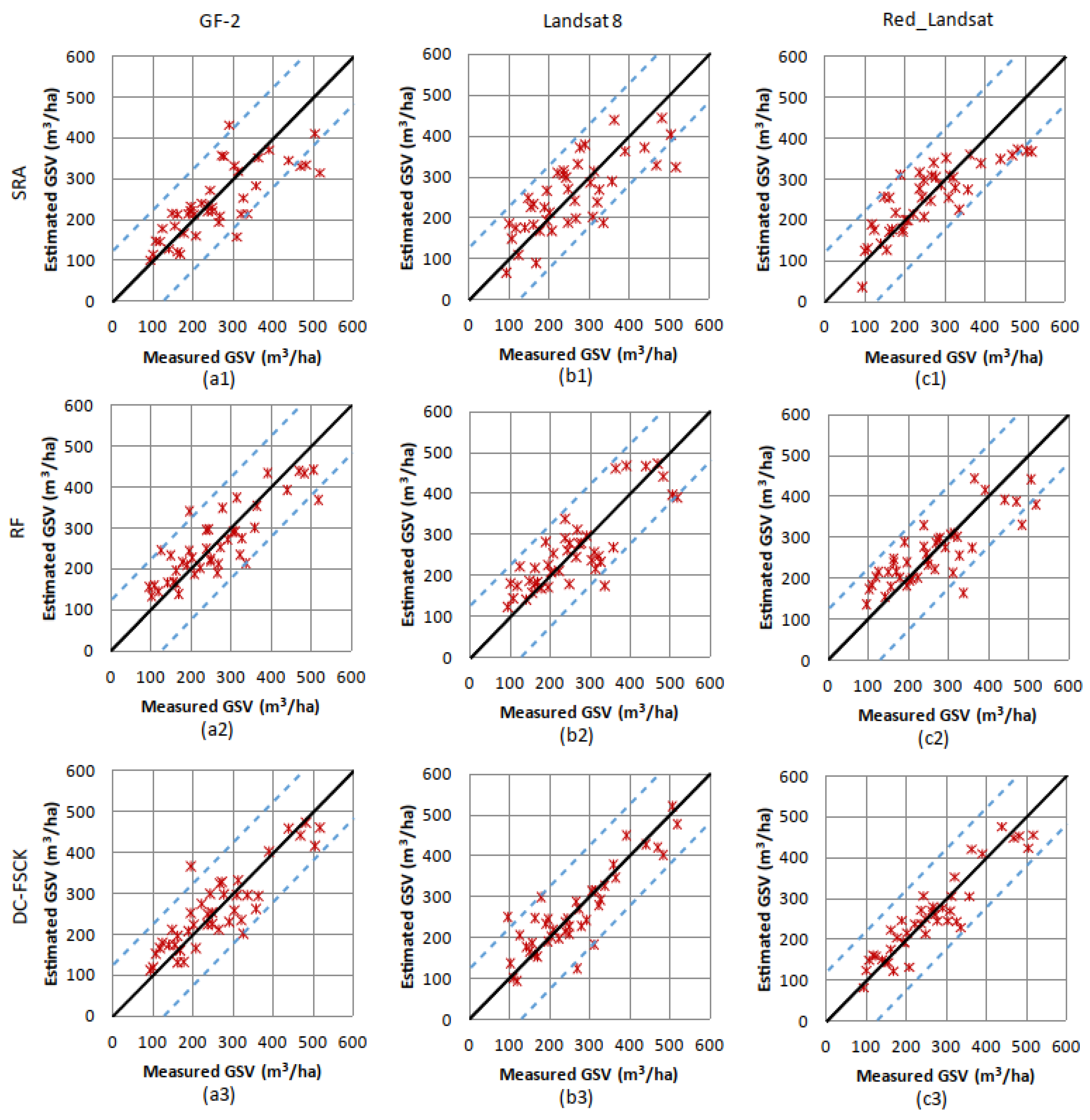
Generally, the estimation residuals should not be larger than 50% of the sample mean. In Figure 3 and Figure 4, the measured and estimated GSV values were compared for Chinese Pine and Larch Plantations, respectively. For Chinese pine, the Stacking model based on the Red_Landsat image and the DC-FSCK variable selection method has the best fitting trend and the maximum estimate, which potentially indicates the highest saturation level (Figure 3(c3)). For the GF-2 and Landsat 8 images, the Stacking and RF model using the variables selected by the DC-FSCK method also have a good fitting trend and a potentially high saturation level (Figure 3(a3,b3)). Although the scatter graphs (Figure 3(c3 vs. a3 and b3)) look similar, the estimation residual absolute values are considerably different, especially for the sample plots with large GSV values. For example, in Figure 3(a3,b3), there are two and four sample plots with their residual absolute values larger than 128.6 m3/ha, respectively. Whereas, in Figure 3(c3), only one sample plot has the residual value close to 128.6 m3/ha.
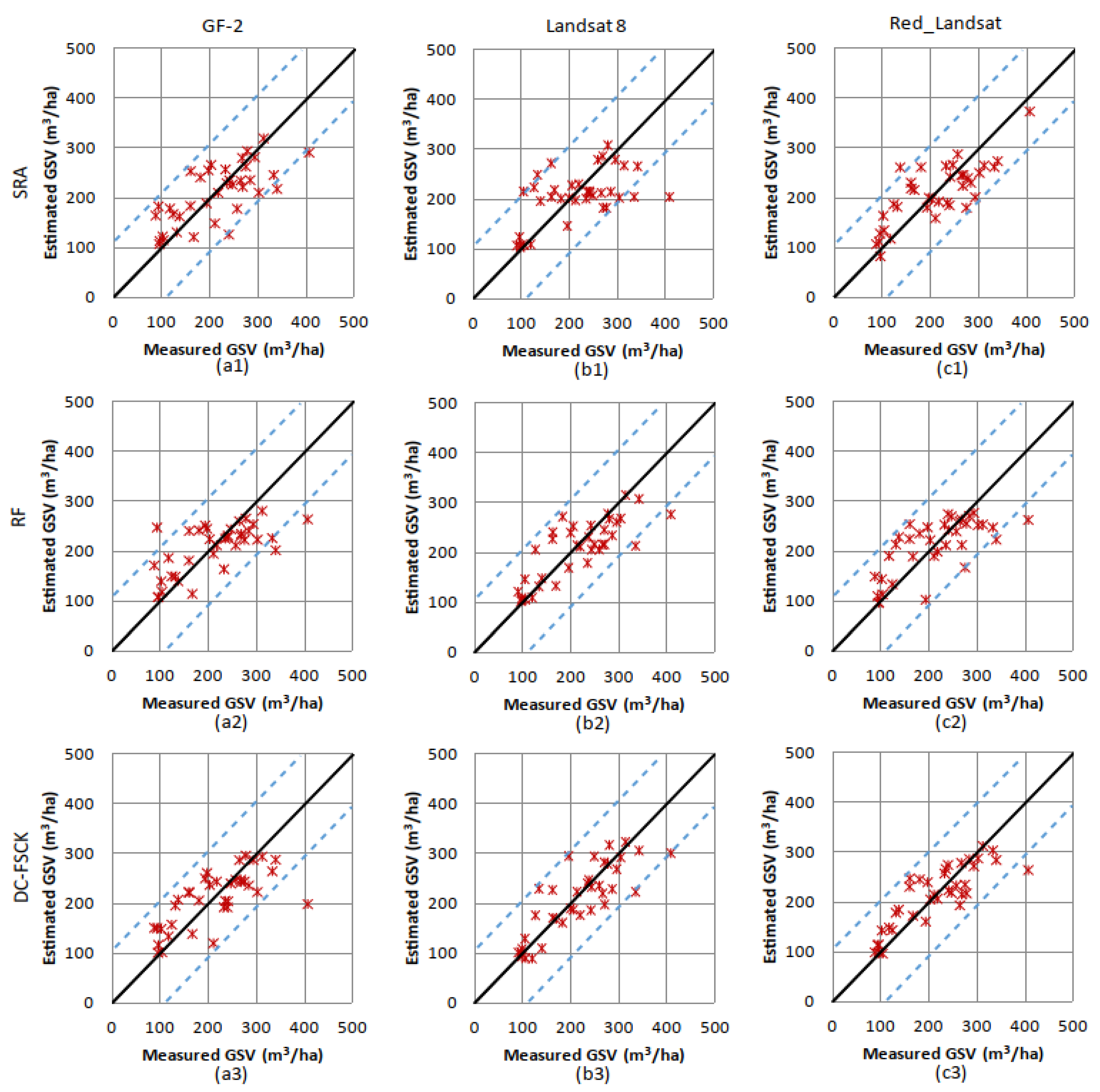
For the larch sample plots, the Red_Landsat image has the best estimation results (Table 6 and Figure 4(c3)), the set of the feature variables selected by DC-FSCK have the potentially highest saturation level, and the Stacking model has the best estimation performance. For the Landsat 8 image (Figure 4(b2,b3)), the sets of the feature variables selected by RF and DC-FSCK also show that most points fit the reference line well, and they have potentially higher saturation levels than that by SRA. The Stacking and RF models have better fitting trends than other models.
In sum, for both Chinese pine and larch sample plots, the fusion image Red_Landsat has richer information than the GF-2 and Landsat 8, and the set of the feature variables selected by DC-FSCK has a potentially higher saturation level than those by SRA and RF. Therefore, the estimation model based on the combination of the Red_Landsat image with the variables selected using the DC-FSCK method has the best fitting trend and the smallest estimation error (Figure 3(c3), Figure 4(c3)).

3.3. Mapping the GSV of Chinese Pine and Larch Plantations

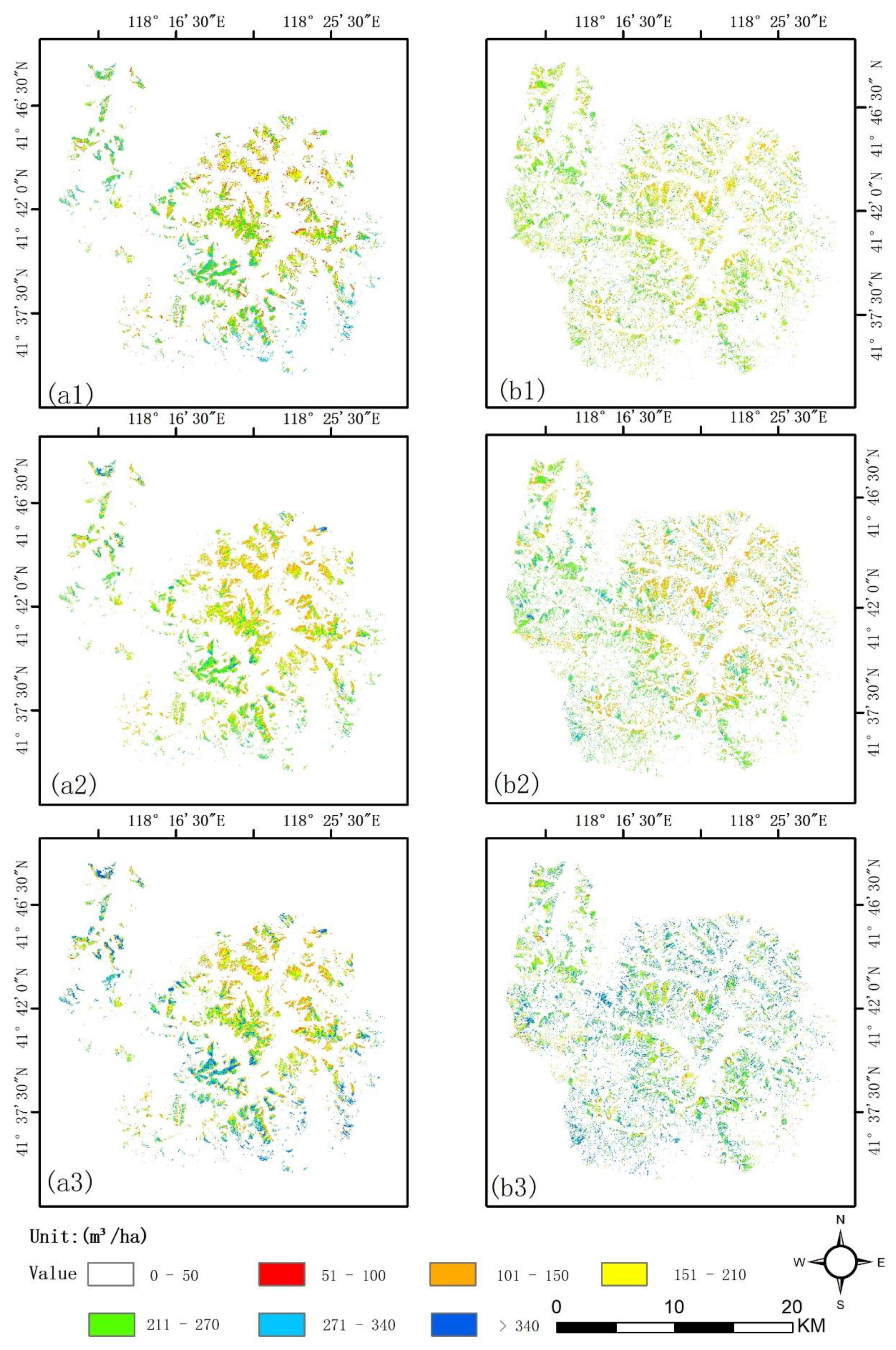
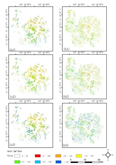
As shown in Figure 5, for both Chinese pine and larch, the GSV estimation models using the variables selected by the DC-FSCK method get more pixels with the GSV values greater than 270 m3/ha than other models (Figure 5(a3) vs. (a1,a2) and (b3) vs. (b1,b2)), indicating that the selection of the key feature variables is important in increasing data saturation levels. It also shows that the sets of the feature variables selected by the DC-FSCK method have potentially higher saturation levels and contain more useful information.

4. Discussion

4.1. The Role of Data Fusion in GSV Estimation

Fusing multispectral and panchromatic images from different optical sensors helps the visual interpretation of vegetation, mainly because it improves spatial resolution [37,40]. This research showed that the fusing data of high-resolution multispectral bands with medium-resolution multispectral images can improve the accuracy of GSV estimation for Chinese pine and larch plantations in northern China. Some studies have proved that the red band performs much better than other bands when using optical images for AGB or GSV estimation [28,31], which is consistent with the finding of this study that the Red_Landsat image fused by the GF-2 red band with the Landsat 8 multispectral data leads to larger R2 and smaller RMSEr values than other fused images, including the fusion image Pan-Landsat.
The spatial information of the 1 m spatial resolution GF-2 image is much richer than that of the 30 m spatial resolution Landsat 8 image. AS shown in Table 5, for Chinese Pine and Larch plantations, more texture variables are selected from the GF-2 images than the Landsat 8 image. But the GF-2 image has no SWIR bands that have a strong relationship with GSV or AGB [13,31]. The fusion image Red_Landsat has both high spatial resolution and SWIR bands and thus resulted in the best performance in the GSV estimation.

4.2. Effective Methods for Improving Spectral Variable Selection and Data Saturation

Different remote sensing feature variables have different saturation and sensitivities to forest GSV estimation. The selected feature variables with low saturation can hardly generate high forest GSV values, so studies should focus on improving the selection of feature variables and increasing the data saturation levels. Although the stratification of forest types and topography can improve the GSV estimation accuracy [13,31], it cannot effectively capture the important and un-correlated feature variables and thus cannot increase the data saturation levels. Therefore, using proper variable selection methods, such as DC-FSCK, is important in increasing data saturation levels. The DC-FSCK can examine the linear and nonlinear relationships between feature variables and GSV and consider the self-correlation and combination effects among the feature variables. The SRA and RF can only select the variables with good linear correlation or importance, but discard the rest variables that might have a high saturation level and contain useful information [19]. Song et al. [19] proposed a spectral variable selection method by integrating Jeffreys–Matusita distance and correlation among feature variables for image classification of wetlands and found that their method offered greater potential than RF. However, their method ignores the combination effects of the feature variables.
This study revealed that based on the fused image Red_Landsat, using the sets of the feature variables selected by the DC-FSCK, RF, and SRA methods, the GSV maximum values of the Chinese pine and larch plantations were about 490 m3/ha and 350 m3/ha, 410 m3/ha and 300 m3/ha, 400 m3/ha and 320 m3/ha, respectively, indicating the corresponding saturation levels. The sets of the spectral variables selected by the DC-FSCK method led to potentially higher saturation level and GSV estimation accuracies than those by RF and SRA. Zhao et al. [31] used the feature variables selected from Landsat Thematic Mapper images by SRA and a spherical model, and obtained the forest biomass saturation values of 159 Mg/ha and 152 Mg/ha for pine (Pinus Massoniana) plantations and broad-leave forests in Zhejiang of Eastern China. Based on the study of Wang et al. [66], the average gravity coefficients of the pine and broad-leave forests in this area were 0.446 g/cm3 and 0.417 g/cm3, respectively. Thus, the authors got GSV saturation values of 356.5 m3/ha and 364.5 m3/ha for the pine and broad-leave forests. The pine plantations are biologically similar to Chinese pine forests in this study. However, the authors resulted in a much smaller GSV saturation value although the mature plantations of Pinus Massoniana in eastern China often have greater per unit GSV value than mature Chinese pine plantations in northern China. This might be mainly because different optical images and spectral variable selection methods were utilized and the data fusion was ignored. Moreover, Long et al. [10] obtained the saturation values of GSV ranging from 140.05 m3/ha to 349.84 m3/ha using a saturation-based multivariate method and quad-polarimetric synthetic aperture radar SAR images for Chinese fir plantations in the Hunan area of south central China. Although the Chinese fir plantations are also biologically similar to the Chinese pine plantations, mature Chinese fir plantations in south central China usually have larger per unit GSV values than the Chinese pine plantations in north China. More importantly, microwave images are less affected by weather conditions such as clouds, fogs and moisture, and SAR is characterized by the capacity to penetrate forest canopies. Thus, the quad-polarimetric SAR images should provide greater potential to obtain higher saturation levels than optical images. However, the GSV saturation values of the Chinese fir plantations obtained by Long et al. [10] are much smaller compared with those of the Chinese pine forests in this study. This might be mainly due to the uncertainties that are induced by the complexity of processing SAR images and the lack of the feature variables that accurately capture the characteristics of the data saturation.

4.3. Selection of Suitable and Stable Estimation Algorithms

This research compared six estimation models based on different data sources of Chinese pine and larch in northern China (Table 6). The results show that the performances of these models vary with tree species, images, and the selected feature variables. For example, when the Landsat 8 image was used for Chinese pine GSV estimation, the MLR model led to higher estimation accuracy than the machine learning algorithms using the variables selected by SRA, and the RF model resulted in smaller RMSEr value using the variables selected by RF. However, when the variables selected by DC-FSCK were used, the SVR model performed best. For the Red_Landsat image, when the variables selected by DC-FSCK were utilized, the Stacking model had RMSEr values of 17.05% and 20.68%, which are 39.1% and 36.4% smaller than those of MLR for Chinese pine and larch, respectively. In addition, previous research results show that the estimation method of relearning based on the prediction results of different basic learners has good estimation accuracy [53]. This conclusion confirms the findings of this study on GSV estimation using the Stacking algorithm.

4.4. Implication of Methods for Improving GSV Estimation of Chinese Pine and Larch Plantations

Optical images often have low saturation levels and thus have low accuracy when they are used for forest AGB or GSV estimation [5,16]. Tree height or canopy height has higher saturation levels and is an important forest stand attribute, so the variables based on height provide great potential for improving AGB or GSV estimation [25,26,28,35]. However, it is expensive to get sufficient photogrammetric and LiDAR data that can be used to extract tree height. Optical images are easily acquired with large-scale coverages, so increasing the saturation level of optical images is a cost-efficient way for GSV estimation. The results of this study show that the multispectral and multispectral image fusion method can improve the performance of GSV estimation and increase the data saturation level by the DC-FSCK method.
The high estimation accuracy of forest GSV depends on many factors, such as forest structure characteristics, the quality of field plot data and images, ancillary data, methods for variable selection, and models used for estimation. The GSV of forest plots with low canopy density and large gaps between canopies is usually overestimated, because bare soils, shrubs and grass under canopies have great influence on the surface reflectance, resulting in the high uncertainty of the GSV estimation [13]. Contrarily, forest plots with high canopy densities and large GSV values often have GSV underestimation, since the optical sensor data cannot capture the vertical structural features of the forest canopies, thus lead to small saturation values [31].
In addition to using the forest canopy structure features, such as tree height and canopy height, there are other ways to improve the GSV estimation accuracy and saturation levels. First, using fused images obtained by integrating high spatial resolution bands with medium spatial resolution multispectral images. In this study, the GF-2 multispectral bands and Landsat 8 multispectral image were fused to obtain new sets of Landsat-like multispectral images. In future studies, data fusion of other optical sensors’ (such as ZY-3 and Sentinel-2, etc.) images should be explored. Secondly, applying a suitable image fusion method. This study used the Gram–Schmidt method to fuse the GF-2 multispectral bands with the Landsat 8 multispectral image. The impact of different fusion methods, such as Wavelet transform, Energy Division transform, and PCA transform on the performance improvement of GSV estimation should be analyzed in future studies. Thirdly, extracting the feature variables that significantly contribute to the estimation improvement of forest GSV, such as texture measures, topographical, phenological and auxiliary data. Current GSV estimation models focus on the use of spectral variables from remote sensing images and only a few reports take phenological features and auxiliary data into account [17,18,33,34]. Future attention should be paid to the consideration of the variables from different data sources.
Moreover, appropriate methods should be further developed to select the significant and un-correlated variables that can lead to high saturation levels and improvement of GSV estimation performance. In this study, DC-FSCK was used to select the feature variables and improved the GSV estimation performance. However, the DC-FSCK method needs to further be refined, such as speeding up the program’s running and simplifying computational complexity. In addition, new estimation models that are relatively simple and easily used and less sensitive to sample size should be developed. In this study, the Stacking showed the best performance for the GSV estimation of both Chinese pine and larch plantations (Table 6). However, this method is very complicated and time-consuming. It requires a set of inputs, such as base-learning and meta-learning algorithms, and optimizing hyperparameters, so the results may vary with different initial inputs. The characteristics of the Stacking should be further investigated in future studies. With the development of machine learning, the process of constructing algorithms is getting simpler and requires less interactions from users. Automatic Machines Learning (AutoML) is intended to automatize the entire process of machine learning, including neural network architecture search, learning algorithm selection, hyperparameter optimization, model evaluation and model application, resulting in end-to-end models. AutoML may also be promising to improve the GSV estimation. Finally, in this study, the proposed method that aims to create, extract and select the significant and un-correlated feature variables to improve the saturation levels and estimation accuracy of GSV for Chinese pine and larch was validated in one study area. In order to evaluate the robustness of this method, further verification is needed in various study areas.

5. Conclusions

This research fused GF-2 multispectral band and Landsat 8 multispectral images to estimate the GSV of Chinese pine and larch plantations in North China. An improved variable selection method DC-FSCK was developed and compared with SRA and RF to screen the feature variables used for modeling. Six models for GSV estimation were compared, which are MLR, kNN, SVR, RF, XGBoost and Stacking. A comparative analysis of the GSV estimation results indicates that (1) fusing the data of high-resolution GF-2 multispectral bands with medium spatial resolution Landsat 8 multispectral image provides more accurate estimates of GSV than those of the high-resolution panchromatic band and medium-resolution multispectral image. The fused image Red_Landsat based on the GF-2 Red band contained the information of both high resolution and SWIR band, and thus performed better than the other fused images (Blue_Landsat, Green_Landsat, and Nir_Landsat) and the original images. The GSV estimation using the Red_Landsat image and the feature variables selected by DC-FSCK had the smallest RMSEr values for both tree species. (2) Different feature variables lead to different data saturation levels. The vegetation indices and texture features extracted from the fused image Red_Landsat showed potentially higher saturation values. Employing a proper variable selection method, such as DC-FSCK, is critical in capturing the canopy structure characteristics of the plantations and thus increasing the data saturation levels. The DC-FSCK examined the nonlinear relationship and combination effects among the spectral variables, so the selected spectral variables resulted in better GSV estimation performance and higher saturation values than those selected by SRA and RF. Based on the Red_Landsat image for Chinese pine, the smallest RMSEr values were 24.85%, 26.10% and 17.05%, respectively, for the variables selected by SRA, RF and DC-FSCK. For larch plantations, the corresponding RMSEr values were 24.11%, 26.75% and 20.68%, respectively. (3) The Stacking performs better than MLR and other machine learning algorithms for the GSV estimation of Chinese pine and larch plantations. For Chinese pine and larch, the average RMSEr values of all the combinations of three datasets (GF-2, Landsat 8, and Red_Landsat image) with three variable selection methods (SRA, RF and DC-FSCK) by the Stacking algorithm were 24.31% and 25.78%, respectively, smaller than those by MLR and other machine learning algorithms.

Supplementary Materials

The following are available online at https://www.mdpi.com/2072-4292/12/5/871/s1, Figure S1: (a) The GF-2 image; (b) the Landsat 8 image; (c) the fusion image Green_Landsat; and (d) the fusion image Red_Landsat. Figure S2: The process of selecting feature variables by the DC-FSCK algorithm.

Author Contributions

Conceptualization, X.L., Z.L. and G.W.; methodology, X.L., Z.L. and H.L.; software, X.L.; validation, X.L., Z.L., J.L. and G.W.; formal analysis, X.L., Z.L. and H.L.; investigation, X.L., Z.L., J.L., H.S., H.L. and M.Z.; resources, X.L., Z.L., J.L. and M.Z.; data processing, X.L., Z.L. and H.S.; original draft, X.L.; review and revision, X.L., Z.L., H.L., H.S. and G.W.; final editing: G.W.; visualization, X.L., Z.L. and J.L.; supervision, H.L., G.W. and H.S.; project administration, X.L. and Z.L.; funding acquisition, H.L. All authors have read and agreed to the published version of the manuscript.

Funding

This study was financially supported by the National Key R&D Program of China project “Research of Key Technologies for Monitoring Forest Plantation Resources” (2017YFD0600900).

Conflicts of Interest

The authors declare no conflict of interest.

References

  1. Brockerhoff, E.G.; Jactel, H.; Parrotta, J.A.; Ferraz, S.F.B. Role of eucalypt and other planted forests in biodiversity conservation and the provision of biodiversity-related ecosystem services. Ecol. Manag. 2013, 301, 43–50. [Google Scholar] [CrossRef]
  2. Carnus, J.; Parrotta, J.; Brockerhoff, E.G.; Arbez, M.; Jactel, H.; Kremer, A.; Lamb, D.; O’Hara, K.; Walters, B. Planted forests and biodiversity. J. For. 2006, 104, 65–77. [Google Scholar]
  3. Cormac, J.O.; Irwin, S.; Byrne, K.A.; O’Halloran, J. The role of planted forests in the provision of habitat: An Irish perspective. Biodivers. Conserv. 2016, 26, 3103–3124. [Google Scholar]
  4. Berger, A.; Gschwantner, T.; Mcroberts, R.E.; Schadauer, K. Effects of Measurement Errors on Individual Tree Stem Volume Estimates for the Austrian National Forest Inventory. For. Sci. 2014, 60, 14–24. [Google Scholar] [CrossRef]
  5. Houghton, R.A. Aboveground forest biomass and the global carbon balance. Glob. Chang. Biol. 2005, 11, 945–958. [Google Scholar] [CrossRef]
  6. Di Cosmo, L.; Gasparini, P.; Tabacchi, G. A national-scale, stand-level model to predict total above-ground tree biomass from growing stock volume. Ecol. Manag. 2016, 361, 269–276. [Google Scholar] [CrossRef]
  7. Krejza, J.; Svˇetlík, J.; Bedná, P. Allometric relationship and biomass expansion factors (BEFs) for above- and below-ground biomass prediction and stem volume estimation for ash (Fraxinus excelsior L.) and oak (Quercus robur L.). Trees 2017, 31, 1303–1316. [Google Scholar] [CrossRef]
  8. Shvidenko, A.; Schepaschenko, D.; Nilsson, S.; Bouloui, Y. Semi-empirical models for assessing biological productivity of Northern Eurasian forests. Ecol. Model. 2007, 204, 163–179. [Google Scholar] [CrossRef]
  9. Wijaya, A.; Kusnadi, S.; Gloaguen, R.; Heilmeier, H. Improved strategy for estimating stem volume and forest biomass using moderate resolution remote sensing data and GIS. J. For. Res. Jpn. 2010, 21, 1–12. [Google Scholar] [CrossRef]
  10. Long, J.; Lin, H.; Wang, G.; Sun, H.; Yan, E. Mapping Growing Stem Volume of Chinese Fir Plantation Using a Saturation-based Multivariate Method and Quad-polarimetric SAR Images. Remote Sens. 2019, 11, 1872. [Google Scholar] [CrossRef] [Green Version]
  11. Zhang, H.; Zhu, J.; Wang, C.; Lin, H.; Long, J.; Zhao, L.; Fu, H.; Liu, Z. Forest Growing Stock Volume Estimation in Subtropical Mountain Areas Using PALSAR-2 L-Band PolSAR Data. Forests 2019, 10, 276. [Google Scholar] [CrossRef] [Green Version]
  12. Santoro, M.; Beaudoin, A.; Beer, C.; Cartus, O.; Fransson, J.E.S.; Hall, R.J.; Pathe, C.; Schmullius, C.; Schepaschenko, D.; Shvidenko, A.; et al. Forest growing stock volume of the northern hemisphere: Spatially explicit estimates for 2010 derived from Envisat ASAR. Remote Sens. Environ. 2015, 168, 316–334. [Google Scholar] [CrossRef]
  13. Lu, D.; Chen, Q.; Wang, G.; Li, G.; Moran, E. A survey of remote sensing-based aboveground biomass estimation methods in forest ecosystems. Int. J. Digit. Earth 2016, 9, 63–105. [Google Scholar] [CrossRef]
  14. Chowdhury, T.A.; Thiel, C.; Schmullius, C. Growing stock volume estimation from L-band ALOS PALSAR polarimetric coherence in Siberian forest. Remote Sens. Environ. 2014, 155, 129–144. [Google Scholar] [CrossRef]
  15. Bilous, A.; Myroniuk, A.; Holiaka, D.; Bilous, S.; See, L.; Schepaschenko, D. Mapping growing stock volume and forest live biomass: A case study of the Polissya region of Ukraine. Environ. Res. Lett. 2017, 12, 105001. [Google Scholar] [CrossRef] [Green Version]
  16. Chen, Q.; Gong, P.; Baldocchi, D.; Tian, Y. Estimating Basal Area and Stem Volume for Individual Trees from LIDAR Data. Photogramm. Eng. Remote Sens. 2007, 73, 1355–1365. [Google Scholar] [CrossRef] [Green Version]
  17. Zheng, S.; Gao, C.; Dang, Y.; Xiang, H.; Zhao, J.; Zhang, Y.; Wang, X.; Guo, H. Retrieval of forest growing stock volume by two different methods using Landsat TM images. Int. J. Remote Sens. 2014, 35, 29–43. [Google Scholar] [CrossRef]
  18. Chrysafis, I.; Mallinis, G.; Siachalou, S.; Patias, P. Assessing the relationships between growing stock volume and sentinel-2 imagery in a Mediterranean forest ecosystem. Remote Sens. Lett. 2017, 8, 508–517. [Google Scholar] [CrossRef]
  19. Song, R.; Lin, H.; Wang, G.; Yan, E.; Ye, Z. Improving selection of spectral variables for vegetation classification of east dongting lake, China, Using a Gaofen-1 image. Remote Sens. 2018, 10, 50. [Google Scholar] [CrossRef] [Green Version]
  20. Sinha, S.; Jeganathan, C.; Sharma, L.K.; Nathawat, M.S. A review of radar remote sensing for biomass estimation. Int. J. Environ. Sci. Technol. 2015, 12, 1779–1792. [Google Scholar] [CrossRef] [Green Version]
  21. Nafiseh, G.; Reza, S.; Ali, M. A review on biomass estimation methods using synthetic aperture radar data. Int. J. Geomat. Geosci. 2011, 1, 776–788. [Google Scholar]
  22. Saatchi, S.; Marlier, M.; Chazdon, L.R.; Clark, D.B.; Russell, A.E. Impact of Spatial Variability of Tropical Forest Structure on Radar Estimation of Aboveground Biomass. Remote Sens. Environ. 2011, 115, 2836–2849. [Google Scholar] [CrossRef]
  23. Solberg, S.; Næsset, E.; Gobakken, T.; Bollandsås, O. Forest Biomass Change Estimated from Height Change in Interferometric SAR Height Models. Carbon Balance Manag. 2014, 9, 5. [Google Scholar] [CrossRef] [PubMed] [Green Version]
  24. Pulliainen, J.; Engdahl, M.; Hallikainen, M. Feasibility of Multi-temporal Interferometric SAR Data for Stand-level Estimation of Boreal Forest Stem Volume. Remote Sens. Environ. 2003, 85, 397–409. [Google Scholar] [CrossRef]
  25. Chen, Q.; Laurin, G.V.; Battles, J.J.; Saah, D. Integration of Airborne Lidar and Vegetation Types Derived from Aerial Photography for Mapping Aboveground Live Biomass. Remote Sens. Environ. 2012, 121, 108–117. [Google Scholar] [CrossRef]
  26. Cao, L.; Coops, N.C.; Innes, J.L.; Sheppard, S.R.J.; Fu, L.; Ruan, H.; She, G. Estimation of forest biomass dynamics in subtropical forests using multi-temporal airborne LiDAR data. Remote Sens. Environ. 2016, 178, 158–171. [Google Scholar] [CrossRef]
  27. Fu, L.; Liu, Q.; Sun, H.; Wang, S.; Li, Z.; Chen, E.; Pang, Y.; Song, X.; Wang, G. Development of a System of Compatible Individual Tree Diameter and Aboveground Biomass Prediction Models Using Error-In-Variable Regression and Airborne LiDAR Data. Remote Sens. 2018, 10, 325. [Google Scholar] [CrossRef] [Green Version]
  28. Li, G.; Xie, Z.; Jiang, X.; Lu, D.; Chen, E. Integration of ZiYuan-3 Multispectral and Stereo Data for Modeling Aboveground Biomass of Larch Plantations in North China. Remote Sens. 2019, 11, 2328. [Google Scholar] [CrossRef] [Green Version]
  29. Gao, Y.; Lu, D.; Li, G.; Wang, G.; Chen, Q.; Liu, L.; Li, D. Comparative analysis of modeling algorithms for forest aboveground biomass estimation in a subtropical region. Remote Sens. 2018, 10, 627. [Google Scholar] [CrossRef] [Green Version]
  30. Zhao, P.; Lu, D.; Wang, G.; Liu, L.; Li, D.; Zhu, J.; Yu, S. Forest aboveground biomass estimation in Zhejiang Province using the integration of Landsat TM and ALOS PALSAR data. Int. J. Appl. Earth Obs. 2016, 53, 1–15. [Google Scholar] [CrossRef]
  31. Zhao, P.; Lu, D.; Wang, G.; Wu, C.; Huang, Y.; Yu, S. Examining spectral reflectance saturation in Landsat imagery and corresponding solutions to improve forest aboveground biomass estimation. Remote Sens. 2016, 8, 469. [Google Scholar] [CrossRef] [Green Version]
  32. Chen, Y.; Li, L.; Lu, D.; Li, D. Exploring bamboo forest aboveground biomass estimation using Sentinel-2 data. Remote Sens. 2019, 11, 7. [Google Scholar] [CrossRef] [Green Version]
  33. Sousa, A.M.O.; Gonçalves, A.C.; Mesquita, P.; da Silva, J.R.M. Biomass estimation with high resolution satellite images: A case study of Quercus rotundifolia. ISPRS J. Photogramm. Remote Sens. 2015, 101, 69–79. [Google Scholar] [CrossRef] [Green Version]
  34. Macedo, F.; Adélia, M.; Ana, C.; José, R.; Marques, D.; Paulo, A.; Ricardo, A. Above-ground biomass estimation for Quercus rotundifolia using vegetation indices derived from high spatial resolution satellite images. Eur. J. Remote Sens. 2018, 51, 932–944. [Google Scholar] [CrossRef] [Green Version]
  35. Ni, W.; Zhang, Z.; Sun, G.; Liu, Q. Modeling the stereoscopic features of mountainous forest landscapes for the extraction of forest heights from stereo imagery. Remote Sens. 2019, 11, 1222. [Google Scholar] [CrossRef] [Green Version]
  36. Chopping, M.; Schaaf, C.B.; Zhao, F.; Wang, Z.; Nolin, A.W.; Moisen, G.G.; Martonchik, J.V.; Bull, M. Forest Structure and Aboveground Biomass in the Southwestern United States from MODIS and MISR. Remote Sens. Environ. 2011, 115, 2943–2953. [Google Scholar] [CrossRef] [Green Version]
  37. Khaleghi, B.; Khamis, A.; Karray, F.O.; Razavi, S.N. Multisensor Data Fusion: A Review of the State-of-the-art. Inf. Fusion 2013, 14, 28–44. [Google Scholar] [CrossRef]
  38. Zhang, J. Multi-source Remote Sensing Data Fusion: Status and Trends. Int. J. Image Data Fusion 2010, 1, 5–24. [Google Scholar] [CrossRef] [Green Version]
  39. Karathanassi, V.; Kolokousis, P.; Ioannidou, S. A comparison study on fusion methods using evaluation indicators. Int. J. Remote Sens. 2007, 28, 2309–2341. [Google Scholar] [CrossRef]
  40. Ehlers, M.; Klonus, S.; Åstrand, P.J.; Rosso, P. Multi-sensor Image Fusion for Pansharpening in Remote Sensing. Int. J. Image Data Fusion 2010, 1, 25–45. [Google Scholar] [CrossRef]
  41. Lu, D.; Batistella, M.E.; de Miranda, E.; Moran, E. A Comparative Study of Landsat TM and SPOT HRG Images for Vegetation Classification in the Brazilian Amazon. Photogram Metr. Eng. Remote Sens. 2008, 74, 311–321. [Google Scholar] [CrossRef] [PubMed] [Green Version]
  42. Wang, H.; Wang, C.; Wu, H. Using GF-2 Imagery and the Conditional Random Field Model for Urban Forest Cover Mapping. Remote Sens. Lett. 2016, 7, 378–387. [Google Scholar] [CrossRef]
  43. Peng, L.; Liu, K.; Cao, J.; Zhu, Y.; Li, F.; Liu, L. Combining GF-2 and RapidEye satellite data for mapping mangrove species using ensemble machine-learning methods. Int. J. Remote Sens. 2019, 41, 813–838. [Google Scholar] [CrossRef]
  44. Ge, S.; Bin, X.; Yunxiang, J.; Shi, C.; Wenbo, Z.; Jian, G.; Hang, L.; Yujing, Z.; Xiuchun, Y. Monitoring wind farms occupying grasslands based on remote-sensing data from China’s GF-2 HD satellite—A case study of Jiuquan city, Gansu province, China. Resour. Conserv. Recycl. 2017, 121, 128–136. [Google Scholar]
  45. Lu, D. The Potential and Challenge of Remote Sensing-based Biomass Estimation. Int. J. Remote Sens. 2006, 27, 1297–1328. [Google Scholar] [CrossRef]
  46. Xie, Z.; Chen, Y.; Lu, D.; Li, G.; Chen, E. Classification of Land Cover, Forest, and Tree Species Classes with ZiYuan-3 Multispectral and Stereo Data. Remote Sens. 2019, 11, 164. [Google Scholar] [CrossRef] [Green Version]
  47. Fan, J.; Lv, J. Sure independence screening for ultrahigh dimensional feature space (with discussion). J. R. Stat. Soc. Ser. B 2008, 70, 849–911. [Google Scholar] [CrossRef] [Green Version]
  48. Li, R.; Zhong, W.; Zhu, L. Feature Screening via Distance Correlation Learning. J. Am. Stat. Assoc. 2012, 107, 1129–1139. [Google Scholar] [CrossRef] [Green Version]
  49. Han, Z.; Jiang, H.; Wang, W.; Li, Z.; Chen, E.; Yan, M.; Tian, X. Forest Above-Ground Biomass Estimation Using KNN-FIFS Method Based on Multi-Source Remote Sensing Data. Sci. Silvae Sincae 2018, 54, 73–82. [Google Scholar]
  50. Zhang, C.; Xie, Z. Object-Based Vegetation Mapping in the Kissimmee River Watershed Using HyMAP Data and Machine Learning Techniques. Wetlands 2013, 33, 233–244. [Google Scholar] [CrossRef]
  51. Zhang, C.; Xie, Z. Combining Object-Based Texture Measures with a Neural Network for Vegetation Mapping in the Everglades from Hyperspectral Imagery. Remote Sens. Environ. 2012, 124, 310–320. [Google Scholar] [CrossRef]
  52. Zhang, C.; Denkaa, S.; Coopera, H.; Deepak, R.M. Quantification of sawgrass marsh aboveground biomass in the coastal Everglades using object-based ensemble analysis and Landsat data. Remote Sens. Environ. 2018, 204, 366–379. [Google Scholar] [CrossRef]
  53. Wang, J.; Xu, J.; Peng, Y.; Wang, H.; Shen, J. Prediction of forest unit volume based on hybrid feature selection and ensemble learning. Evol. Intell. 2019, 4, 21–32. [Google Scholar] [CrossRef]
  54. Chen, T.; Guestrin, C. XGBoost: A Scalable Tree Boosting System. In Proceedings of the 22nd ACM SIGKDD International Conference on Knowledge Discovery and Data Mining, ACM, San Francisco, CA, USA, 13–17 August 2016. [Google Scholar]
  55. Wang, J.; Gribskov, M. IRESpy: An XGBoost model for prediction of internal ribosome entry sites. BMC Bioinform. 2019, 20, 409. [Google Scholar] [CrossRef] [PubMed]
  56. Wu, D.; Lin, C.; Huang, J.; Zeng, Z. On the Functional Equivalence of TSK Fuzzy Systems to Neural Networks, Mixture of Experts, CART, and Stacking Ensemble Regression. IEEE Trans. Fuzzy Syst. 2019, 10, 1109. [Google Scholar] [CrossRef] [Green Version]
  57. Wan, S.; Yang, H. Comparison among Methods of Ensemble Learning. In Proceedings of the 2013 International Symposium on Biometrics and Security Technologies, Chengdu, China, 2–5 July 2013. [Google Scholar]
  58. Tao, Y.; Peng, Y.; Jiang, Q.; Li, Y.; Fang, S.; Gong, Y. Remote Detection of Critical Growth Stages in Rapeseed Using Vegetation Spectral and Stacking Combination Method. J. Geomat. 2019, 44, 20–23. [Google Scholar]
  59. Li, W.; Ma, C.; Jin, D.; Hui, J. Sustainable Forest Management Model of Wangyedian Experimental Forest Farm in Karaqin Banner. Inn. Mong. For. Investig. Des. 2016, 6, 47–50. [Google Scholar]
  60. Wu, C.; Ma, C. Struggle for sixty years, dream and flourishing industry—Record of development of Wangye Dian Experimental Forest Farm in Chifeng. Land Green. 2015, 7, 16–19. [Google Scholar]
  61. Soenen, S.A.; Peddle, D.R.; Coburn, C.A. SCS+C: A modified Sun-canopy-sensor topographic correction in forested terrain. IEEE Trans. Geosci. Remote Sens. 2005, 43, 2148–2159. [Google Scholar] [CrossRef]
  62. Li, G.; Peng, H.; Zhang, J.; Zhu, L. Robust rank correlation based screening. Ann. Stat. 2012, 40, 1846–1877. [Google Scholar] [CrossRef] [Green Version]
  63. Shao, X.; Zhang, J. Martingale difference correlation and its use in high dimensional variable screening. J. Am. Stat. Assoc. 2014, 109, 1302–1318. [Google Scholar] [CrossRef]
  64. Sz’ekely, G.J.; Rizzo, M.L.; Bakirov, N.K. Measuring and testing dependence by correlation of distances. Ann. Stat. 2007, 35, 2769–2794. [Google Scholar] [CrossRef]
  65. Sun, H.; Wang, Q.; Wang, G.; Lin, H.; Luo, P.; Li, J.; Zeng, S.; Xu, X.; Ren, L. Optimizing kNN for Mapping Vegetation Cover of Arid and Semi-Arid Areas Using Landsat images. Remote Sens. 2018, 10, 1248. [Google Scholar] [CrossRef] [Green Version]
  66. Wang, G.; Oyana, T.; Zhang, M.; Adu-Prah, S.; Zeng, S.; Lin, H.; Se, J. Mapping and spatial uncertainty analysis of forest vegetation carbon by combining national forest inventory data and satellite images. For. Ecol. Manag. 2009, 258, 1275–1283. [Google Scholar] [CrossRef]
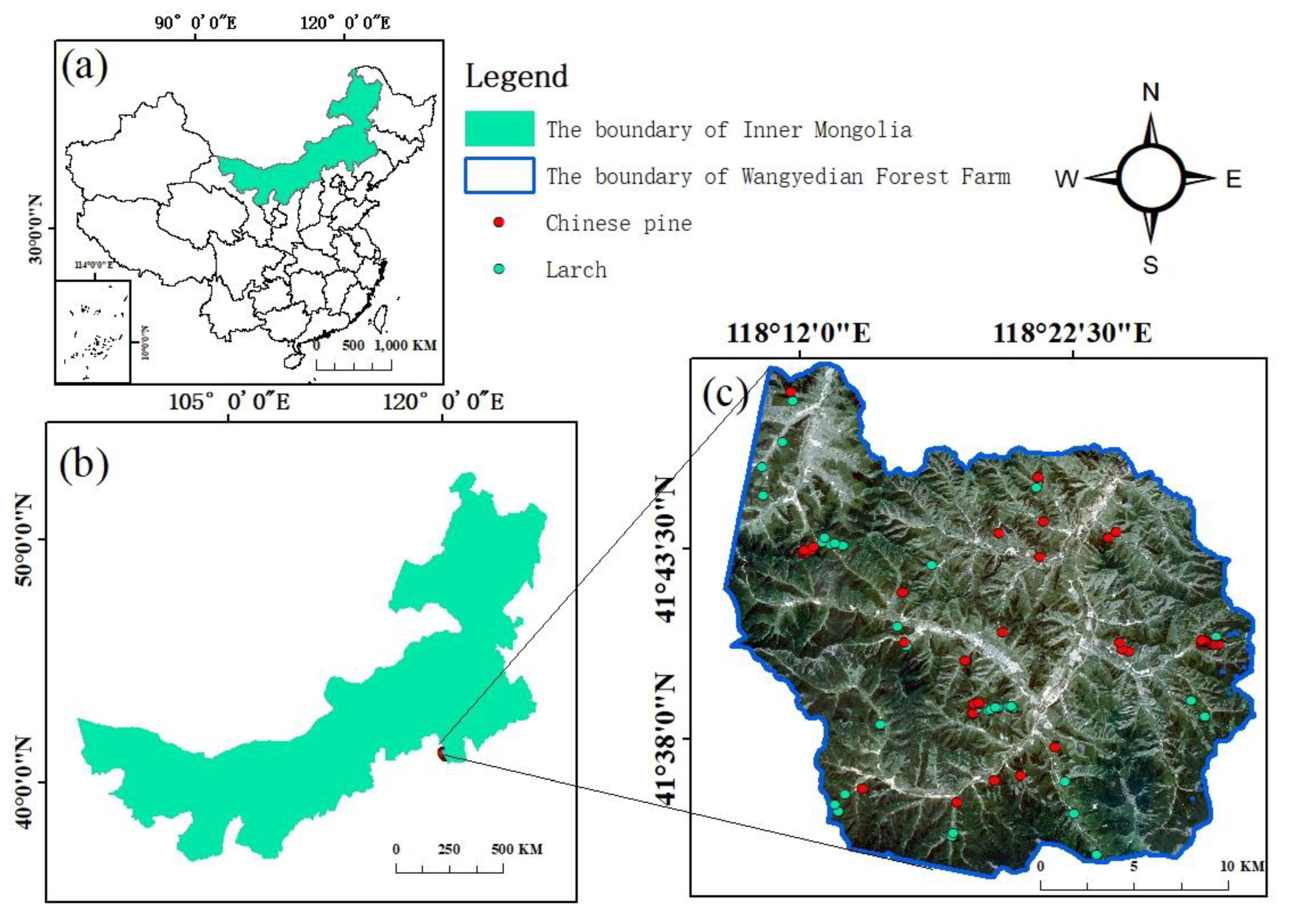
Figure 1. (a) and (b) The location of the study area in North China and Inner Mongolia; and (c) the spatial distribution of larch and Chinese pine plots.
Remotesensing 12 00871 g001
Figure 2. Methodological framework of forest GSV estimation for Chinese pine and larch plantations.
Remotesensing 12 00871 g002
Figure 3. The scatter graphs between the observed and estimated GSV values of the Chinese pine plots using three datasets and three variable screening methods (SRA, RF, and DC-FSCK): (a,b,c) are the GSV estimated by the GF-2, Landsat 8, and Fusion image Red_Landsat, respectively; (1,2,3) are the GSV estimated using the variables selection methods SRA, RF, and DC-FSCK, respectively. Each graph corresponds to the best estimation model with the smallest RMSEr value for each data scenario in Table 6. The black diagonal line is the theoretical best fit reference line, and the blue parallel dashed lines are the estimation residual reference lines with a 50% deviation from the sample mean.
Remotesensing 12 00871 g003
Figure 4. The scatter graphs between the observed and estimated GSV values of the larch plots using three dataset and three variable screening methods (SRA, RF, and DC-FSCK): (a,b,c) are the GSV estimated by the GF-2, Landsat 8, and Fusion image Red_Landsat, respectively; (1,2,3) are the GSV estimated using three variable screening methods SRA, RF, and DC-FSCK, respectively. Each graph corresponds to the best estimation model with the smallest RMSEr value for each data scenario in Table 6. The black diagonal line is the theoretical best fit reference line, and the blue parallel dashed lines are the estimation residual reference lines with a 50% deviation from the sample mean.
Remotesensing 12 00871 g004
Figure 5. The GSV maps of (a1–a3) Chinese pine and (b1–b3) larch plantations in the study area estimated based on the fusion image Red_Landsat using the variables selected by SRA, RF, and DC-FSCK method, respectively. Each map corresponds to the best estimation model with the smallest RMSEr value for each data scenario in Table 6.
Remotesensing 12 00871 g005
Table 1. Tree GSV equations of Chinese pine and larch.
Tree SpeciesGSV EquationsRemarks
LarchV = −0.001498 + 0.00007 × D^2 + 0.000901 × H + 0.000032 × H × D^2V: GSV
D: DBH
H: Tree Height
Chinese pineV = 0.013464 − 0.001967 × D + 0.000089 × D^2 + 0.000628 × D × H + 0.000032 × H × D^2 − 0.003173 × H
Table 2. The GSV statistics of sample plots.
Year of Field MeasurementsNumber of
Plots
GSV Range
(M3/ha)
Mean
(M3/ha)
Standard
Deviation
Chinese pine20174291.97~514.96257.15112.63
Larch20173787.44~405.56211.6981.51
Table 3. Vegetation indices used in this research.
Vegetation IndicesDefinitions
Simple two-band ratiosRVIi = Bandi/Bandj, i, j = 2, …, 7, i ≠ j
Difference vegetation indicesDVIij = Bandi − Bandj, i, j = 2, …, 7, i ≠ j
Normalized difference vegetation indexNDVI = (Nir − Red)/(Nir + Red)
NDVI563 = (Nir + SWIR1 − Green)/(Nir + SWIR1 + Green)
Similar normalized difference vegetation indicesNDVI ij = (Bandi − Bandj)/(Bandi + Bandj),
i, j = 2, …, 7, i ≠ j, Not including NDVI.
Soil adjusted vegetation indicesSAVI i = (Nir − Red)(1 + i)/(Nir + Red + i),
i = 0.1, 0.25, 0.35, 0.5
Atmospherically resistant vegetation indexARVI = (Nir − (2 × Red − Blue))/(Nir + (2 × Red − Blue))
Enhanced vegetation indexEVI = 2.5 × (Nir − Red)/(Nir + 6 × Red − 7.5 × Blue + 1)
Triangular vegetation indexTVI = 0.5 × (120×(Nir − Green) − 200 × (Red − Green))
Modified simple ratioMSR = (Nir/Red − 1)/SQRT(Nir/Red + 1)
Modified Soil adjusted vegetation indexMSAVI = ((2× Nir + 0.25) − SQRT((2× Nir + 0.25)^2 − 8×(Nir − Red)))/2
Perpendicular vegetation indexPVI = 0.939× Nir − 0.344 × Red + 0.09
Table 4. Summary of RMSE, R2, and Adjusted R2 for estimating GSV of Chinese Pine and Larch Plantations using five fusion datasets based on SRA.
Blue_LandsatGreen_LandsatRed_LandsatNir_LandsatPan_Landsat
Chinese pine
RMSE(m3/ha)64.8668.0563.3476.7274.85
R20.70100.66200.70700.55900.5695
Adjusted R2 0.66800.63500.68400.53600.5476
larch
RMSE(m3/ha)57.3161.9856.4459.7261.76
R20.53300.43800.73600.49300.4392
Adjusted R2 0.50600.42200.71600.46300.4231
Table 5. Spectral variables selected by different methods for forest GSV estimation (Note: M—mean, V—variance, H—homogeneity, Con—contrast, D—dissimilarity, E—entropy, S—second moment, Cor—correlation).
Tree SpeciesDatasetsMethodsSpectral Variables
Chinese pineGF-2SRARed_S, Blue, Blue_ Cor
RFBlue, Blue_M, Green_Cor, Green_D, Nir_Con,
Blue _Con, NDVI23
DC-FSCKBlue_M, NDVI13, NDVI12, NDVI24, RVI24
Landsat 8SRANir_E, RVI24, ND47
RFBlue, NDVI57, SWIR2_Cor, RVI35, NDVI56, NDVI35, RVI24
DC-FSCKGreen, Red_Con, RVI57, NDVI24
Red_LandsatSRABlue_M, Blue_H, Coastal _Cor
RFBlue_M, Coastal _M, SWIR2_E, Green_S, DVI34, Blue_S, SWIR2_M, NDVI34
DC-FSCKBlue_M, Green_Dis, Green_S, SWIR2_H, Red_H, SAVI0.25, Coastal _S
LarchGF-2SRAND13, ARVI, RVI34
RFBlue, ARVI, RVI14, Blue_M, Green, RVI24, NDVI14
DC-FSCKBlue, Nir_M, Nir_E, Nir_D, Green_Cor, Red_H, ARVI
Landsat 8SRADVI34, Red_E, Blue_H
RFNDVI67, RVI67, DVI46, DVI24, DVI26, SWIR1_M
DC-FSCKMSR, RVI23, RVI34, Blue_H, RVI27, SAVI0.35
Red_LandsatSRARVI27, EVI, Green_V
RFDVI34, RVI67, SWIR2_M, NDVI57, Blue_M, RVI45, Red_M, NDVI35
DC-FSCKMSR, Blue_M, Coastal _M, Nir_Cor, Nir_V, Green_Dis, MSAVI, SAVI0.1, NDVI46
Table 6. Summary of the Adjusted R2 and RMSEr for GSV estimation of Chinese Pine and Larch Plantations using three variable selection methods and six estimation models based on three datasets (Note: The numbers in bold indicate the model with the greatest Adjusted R2 and smallest RMSEr value in the same data scenario).
Tree SpeciesData ScenariosVariable Selection MethodsPerformance Evaluation of Six Models
MLRkNNSVRRFXGBoostStacking
Adjusted R2RMSEr (%)Adjusted R2RMSEr (%)Adjusted R2RMSEr (%)Adjusted R2RMSEr (%)Adjusted R2RMSEr (%)Adjusted R2RMSEr (%)
Chinses pineGF-2SRA0.4756 30.170.4237 31.620.3591 33.350.4593 30.630.539328.280.5307 28.74
RF0.3351 32.130.2401 34.350.3948 30.660.599924.930.5744 25.710.5825 25.17
DC-FSCK0.3222 33.380.6687 23.340.6005 25.630.5266 27.900.5811 26.240.722621.35
Landsat 8SRA0.525728.690.2247 36.680.3837 32.700.4631 30.530.5192 28.890.5244 28.83
RF0.3780 31.080.2335 34.500.2783 33.480.611224.570.5380 26.790.6066 24.74
DC-FSCK0.3821 32.310.7209 21.720.731521.300.6978 22.600.7172 21.860.7234 21.56
Fusion imagery:
Red_Landsat
SRA0.6189 25.720.5964 26.470.644324.850.6383 25.050.6255 25.490.6356 25.19
RF0.4833 27.910.0676 37.490.2754 33.050.548026.100.5327 26.540.5458 26.17
DC-FSCK0.4956 27.990.7963 17.780.5740 25.720.4568 29.050.4757 28.540.812717.05
LarchGF-2SRA0.1937 32.660.3857 28.500.1881 32.770.3590 29.120.466826.560.4583 27.33
RF−0.0078 34.220.0785 32.730.0635 32.990.365227.010.1768 30.930.3613 27.25
DC-FSCK−0.0578 36.080.3971 26.470.0328 33.530.3486 27.510.1533 31.370.406225.72
Landsat 8SRA0.2401 31.700.246731.560.2054 32.420.0340 36.140.0045 37.260.2457 31.85
RF0.2802 29.42−0.0415 35.380.2657 29.710.563823.210.5543 24.310.5612 23.37
DC-FSCK0.0869 33.130.570023.130.2114 30.790.3774 27.360.2867 29.280.5602 23.52
Fusion imagery:
Red_Landsat
SRA0.560624.110.3175 30.040.5028 25.640.3039 30.340.3781 28.680.5116 25.32
RF0.1572 30.750.2239 29.510.2092 29.790.362226.750.2747 28.530.3550 26.96
DC-FSCK0.0240 32.500.5649 21.700.4665 24.020.3984 25.510.4209 25.030.604720.68