X-Net-Based Radar Data Assimilation Study over the Seoul Metropolitan Area


Abstract
:
1. Introduction
2. Data and Experimental Methods
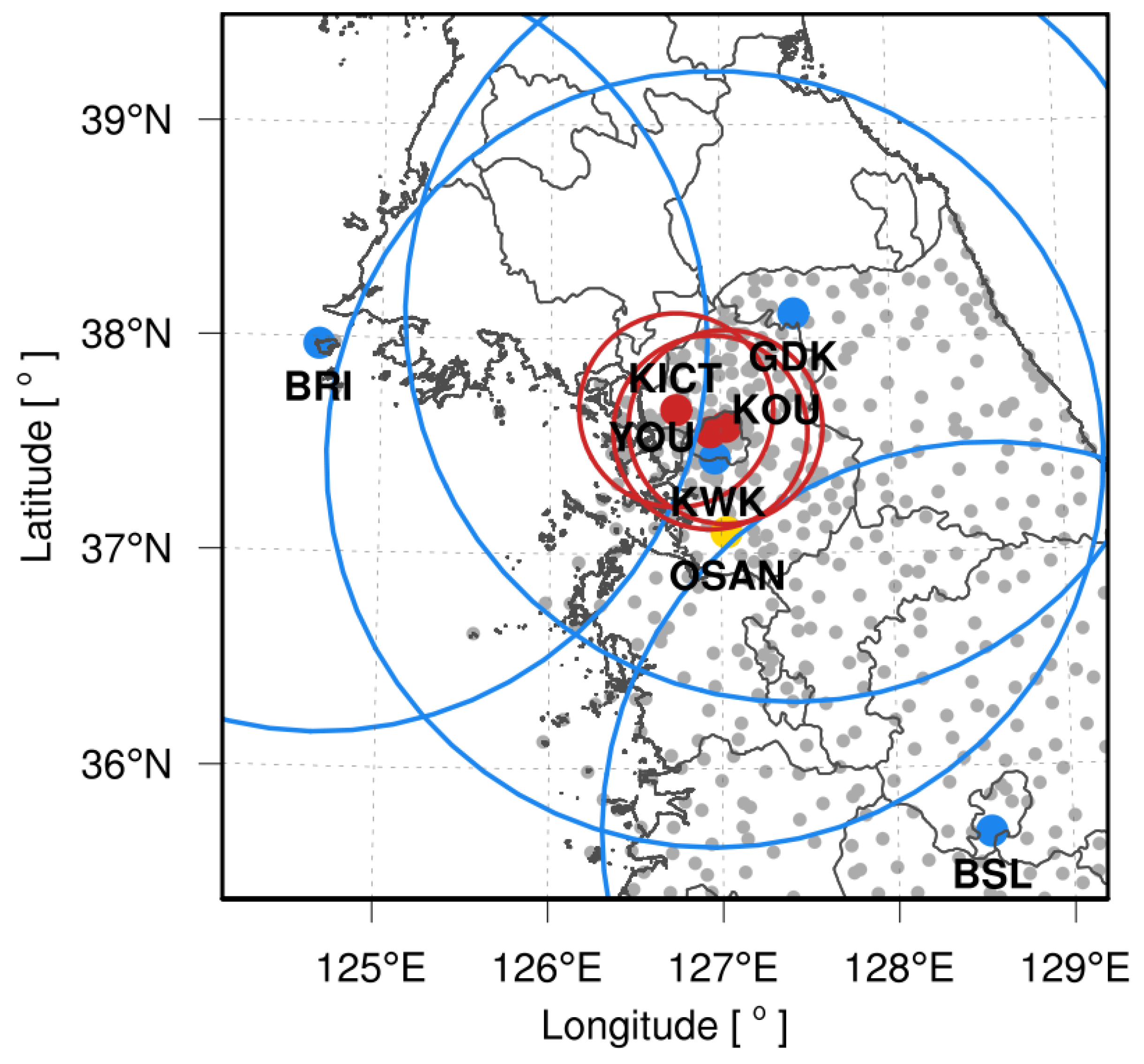
2.1. Observation Data
2.2. WRF 3D-Var Assimilation System
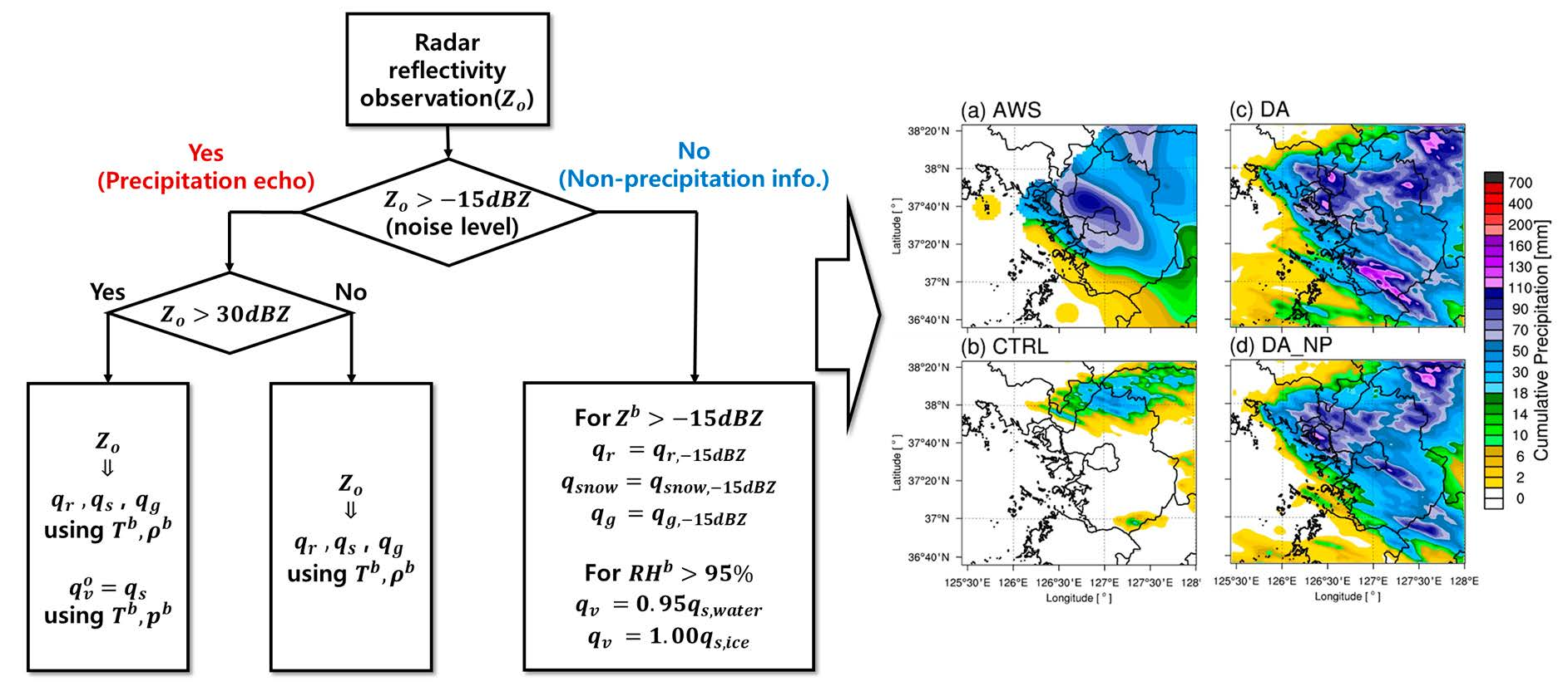
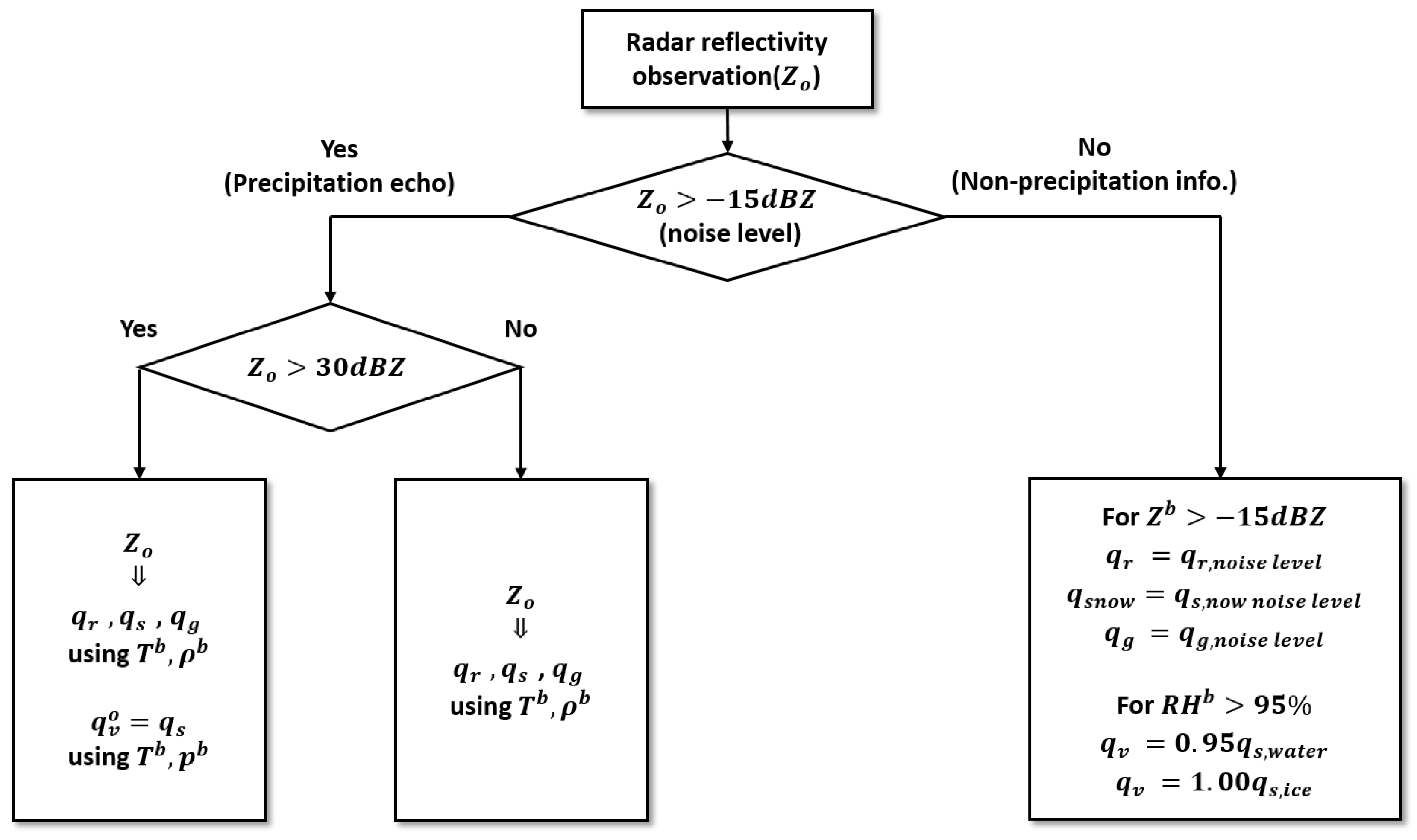
2.3. Radar Observation Operator
2.3.1. Radar Reflectivity Observation Operator
2.3.2. Doppler Radial Velocity Observation Operator
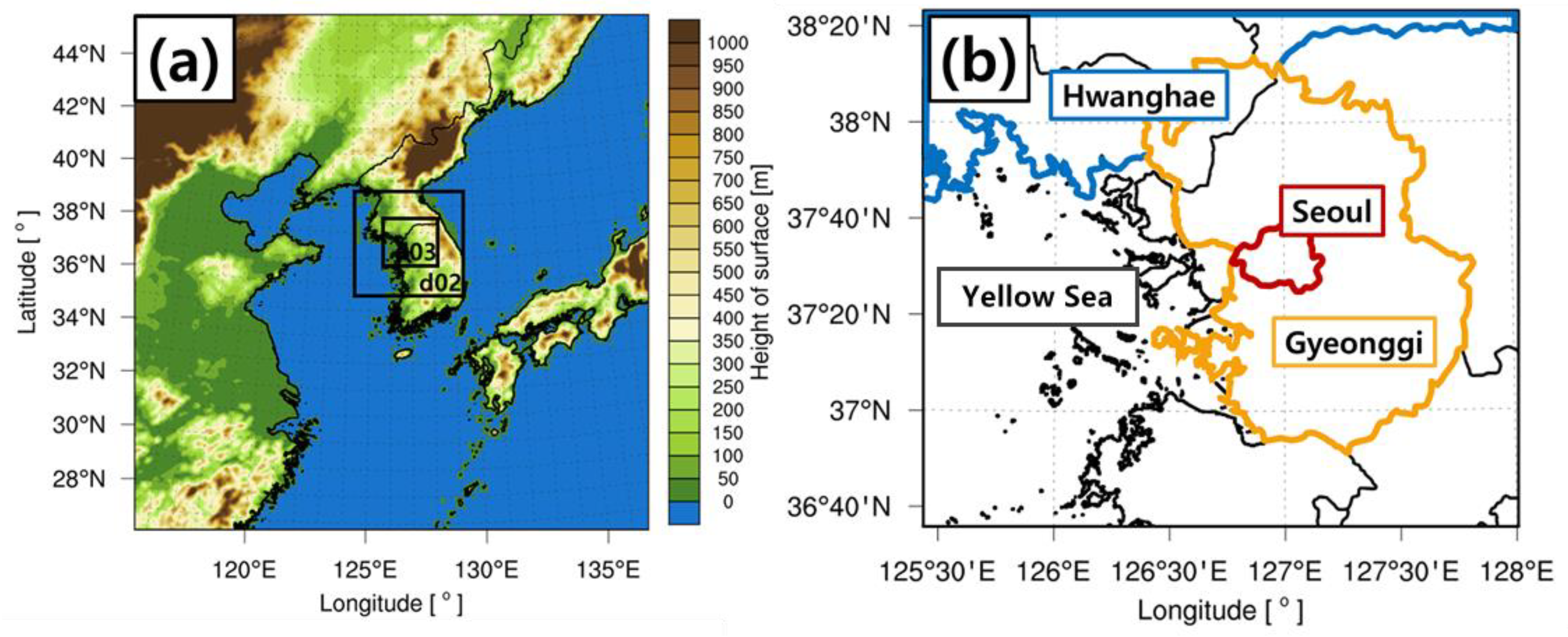
2.4. Model Configuration and Experimental Design
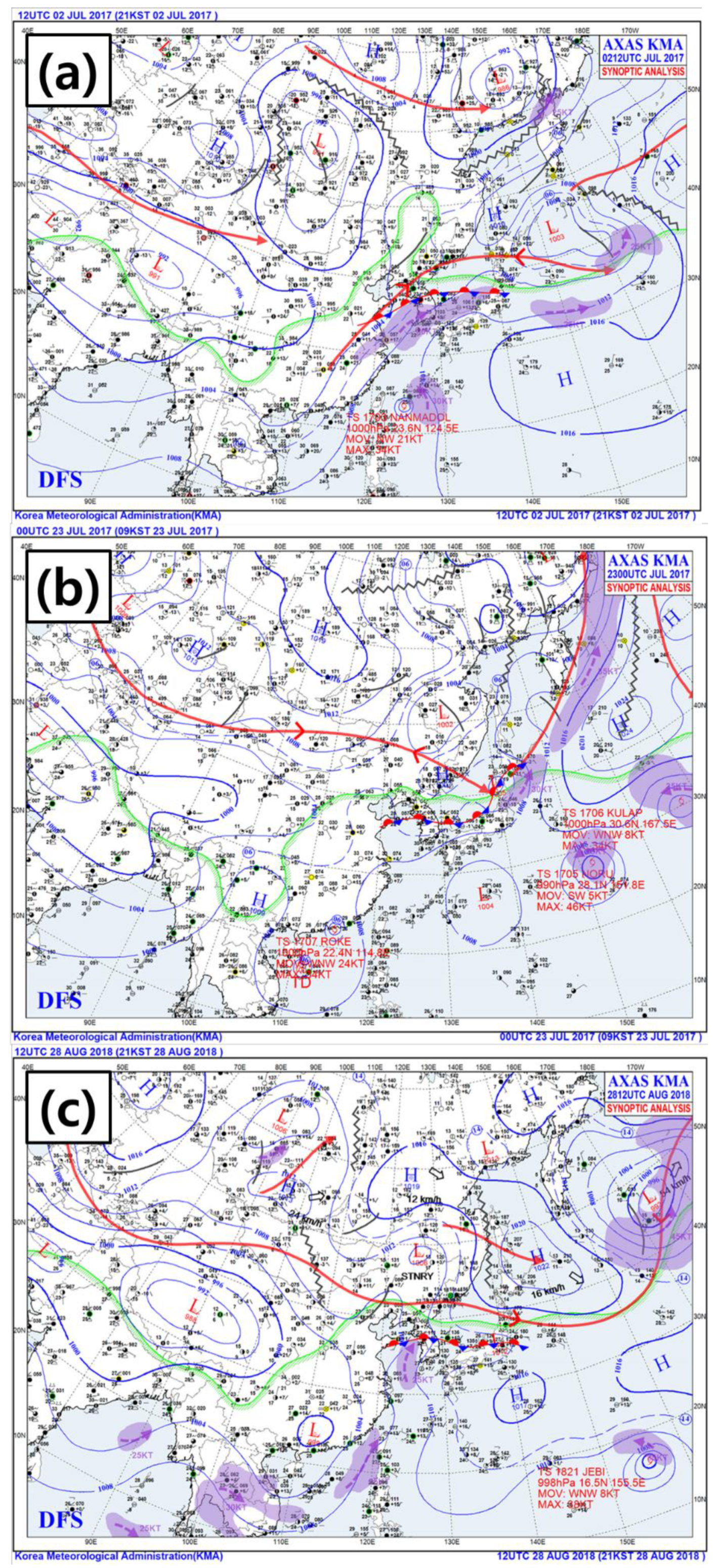
2.5. Description of the Cases
2.6. Evaluation Parameters
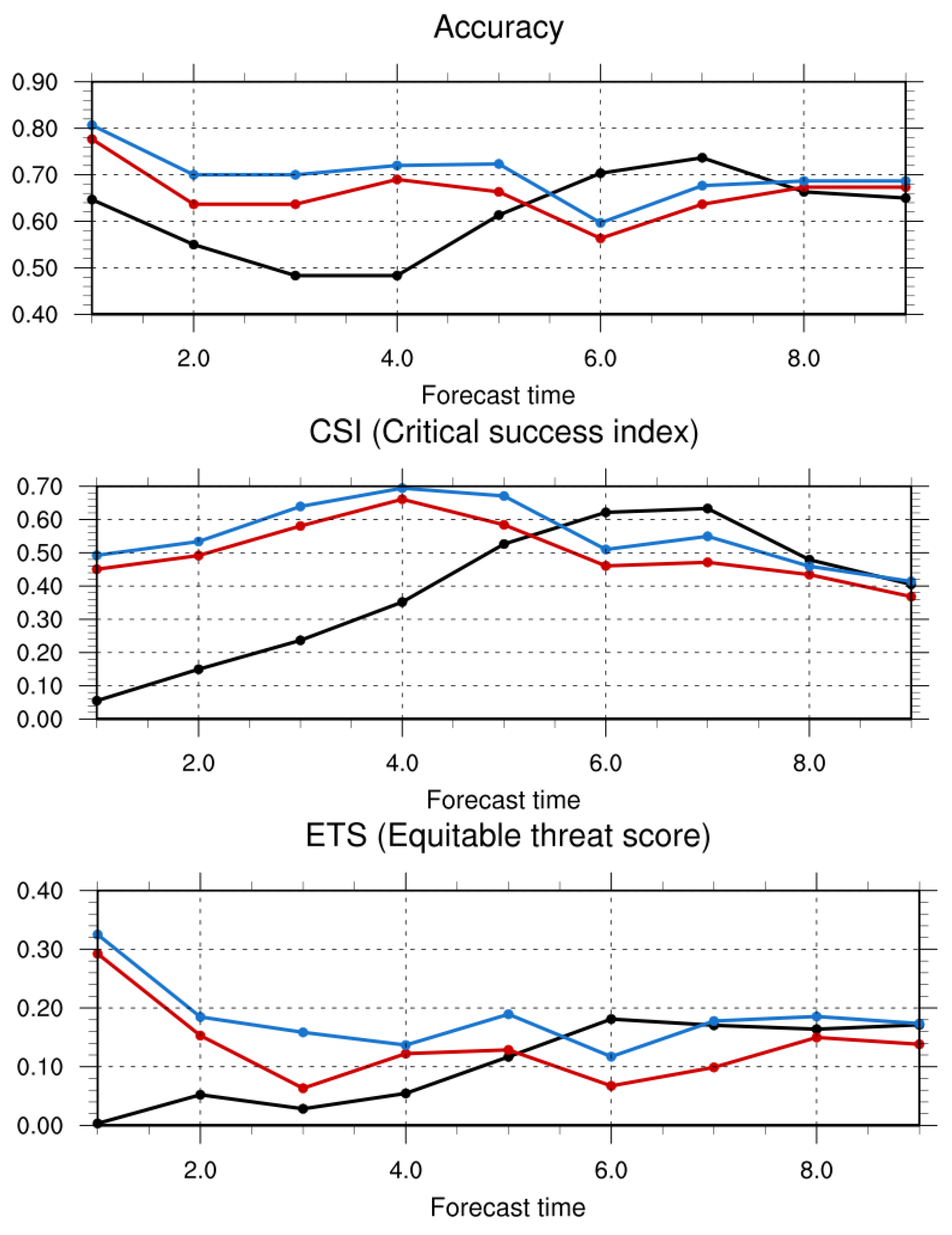
2.6.1. Accuracy Verification
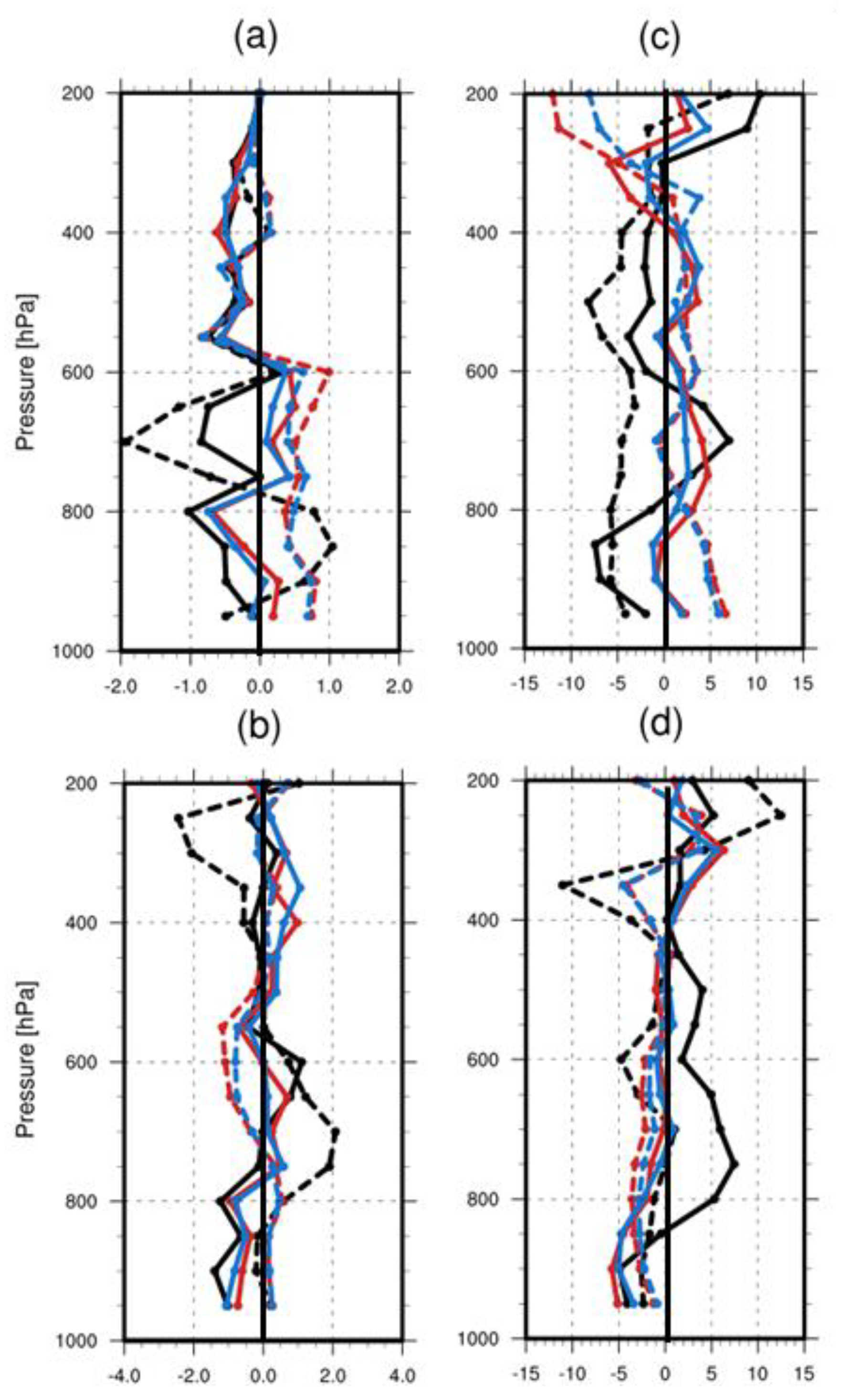
2.6.2. Space- and Time-Averaged Comparison Fields
3. Results
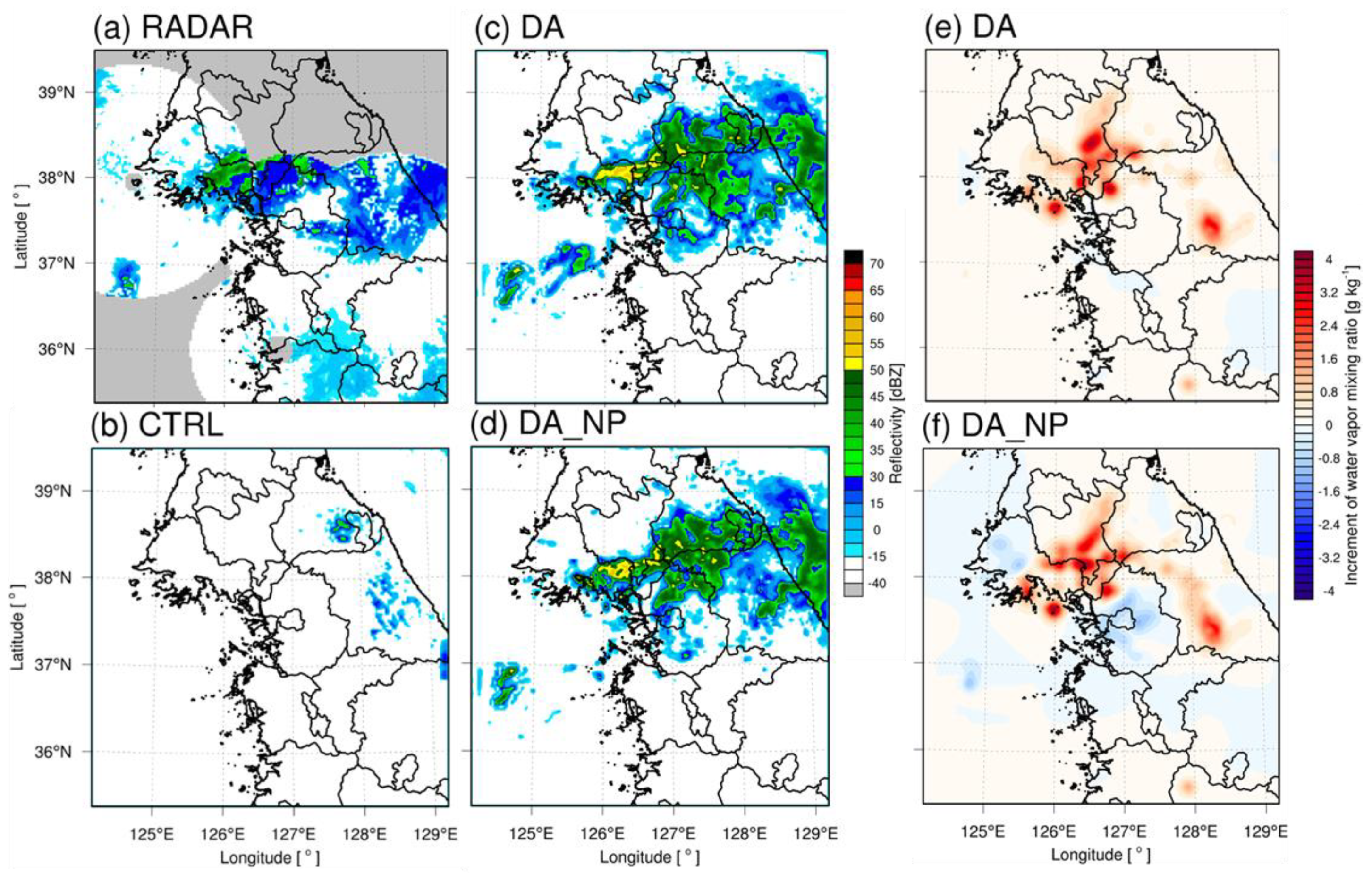
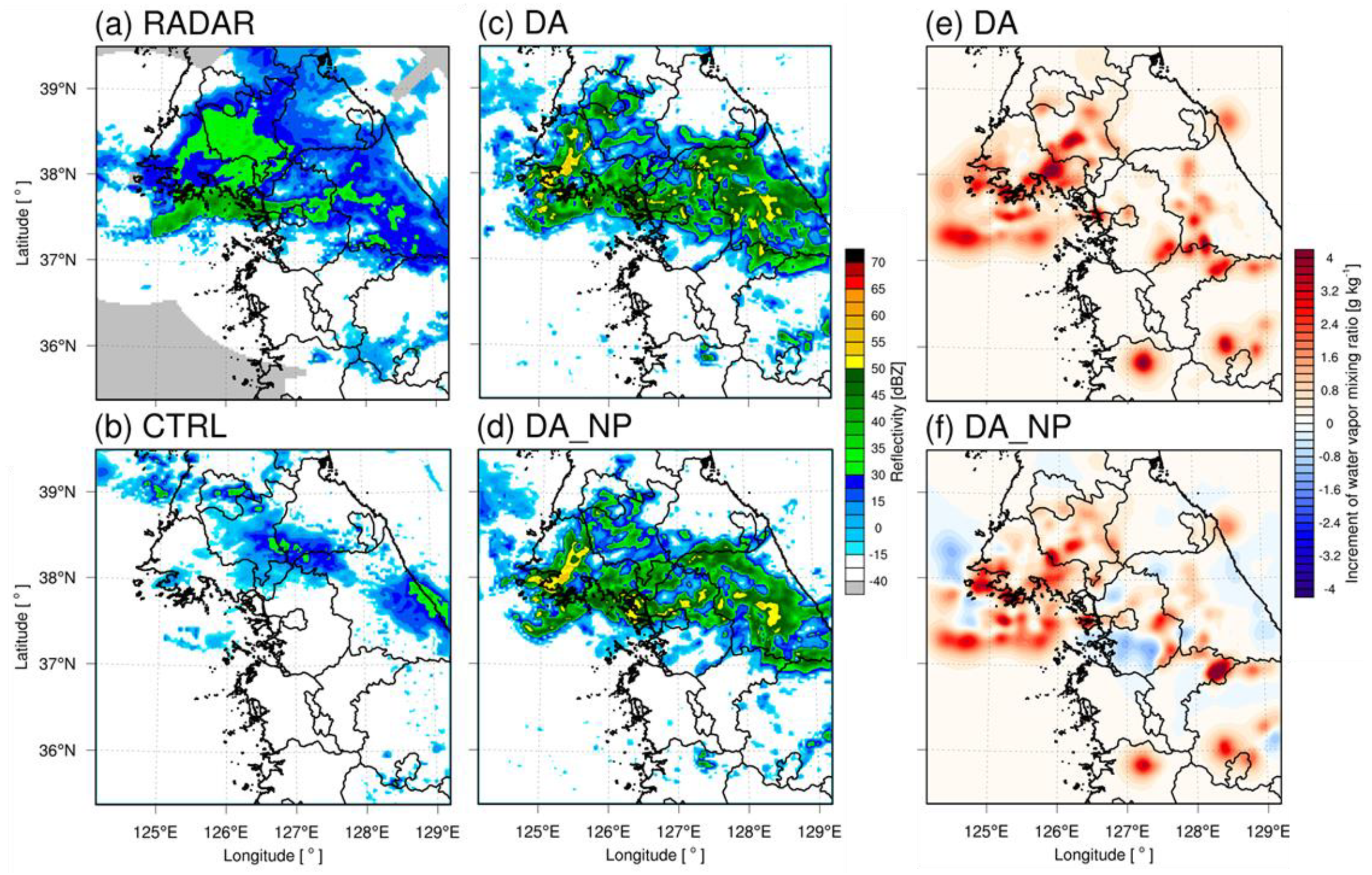
3.1. Increment of the Analysis Field
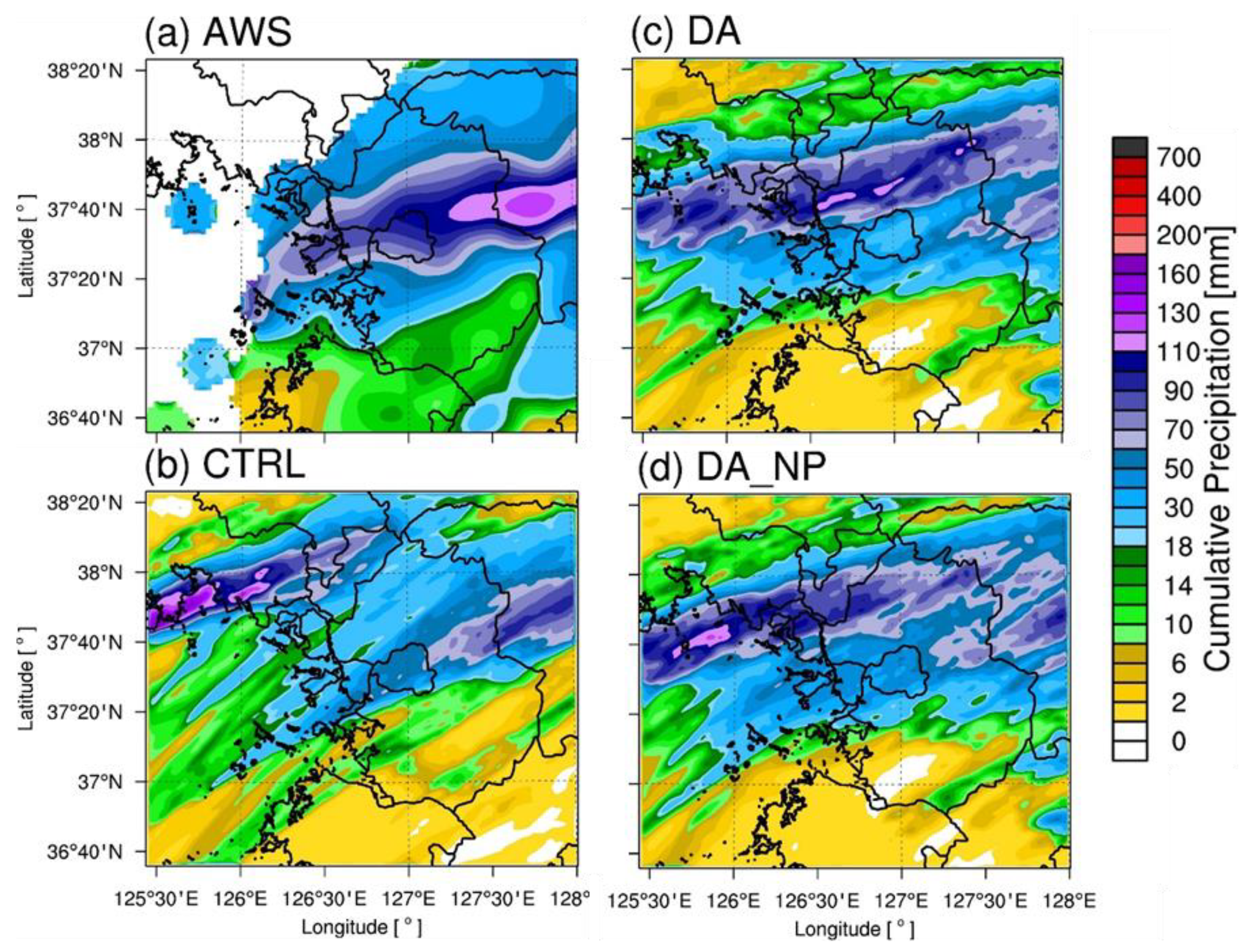
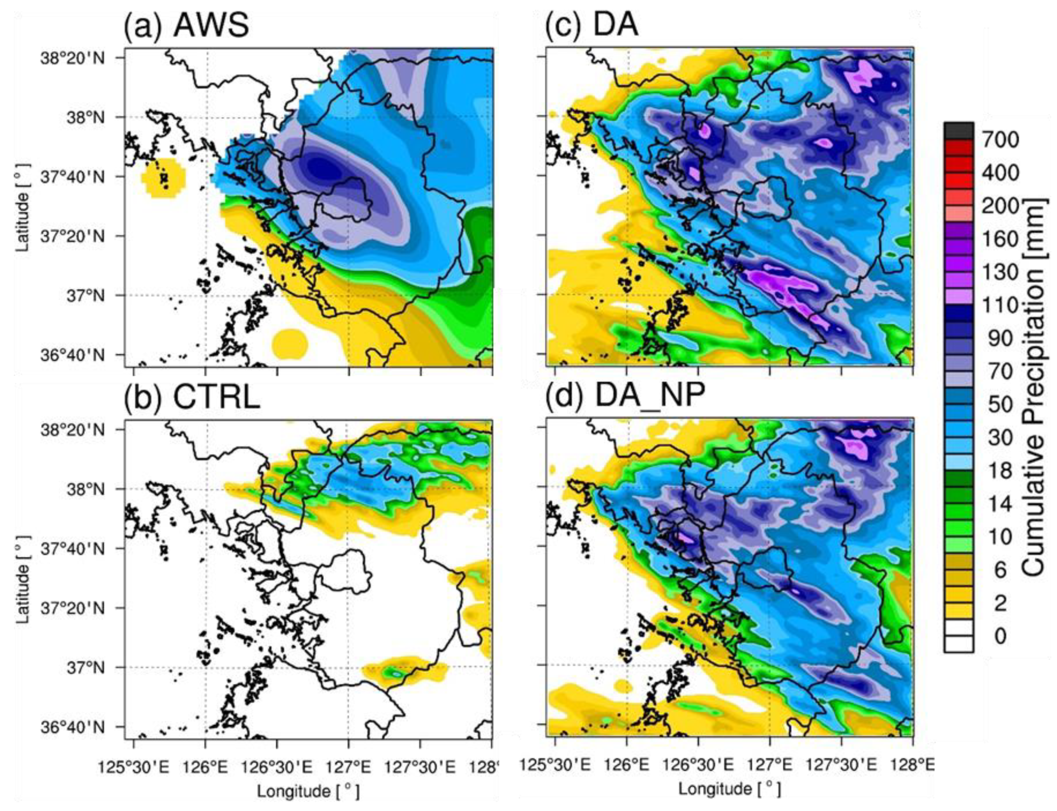
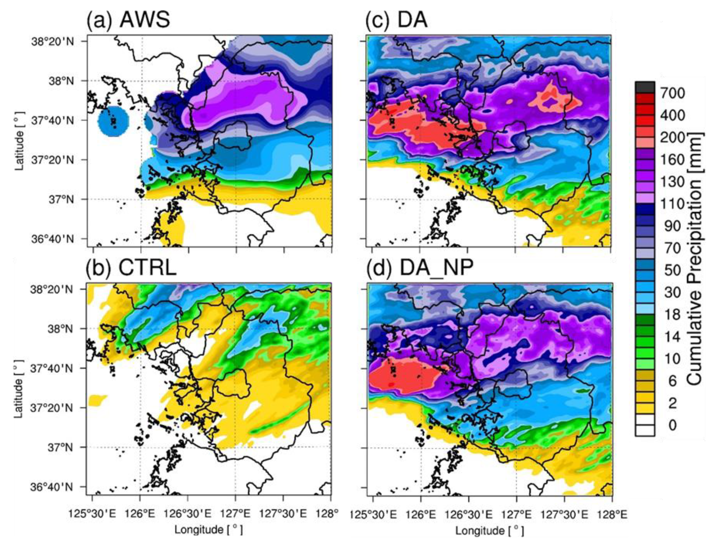
3.2. Distribution of the Cumulative Precipitation
3.3. Model Verification
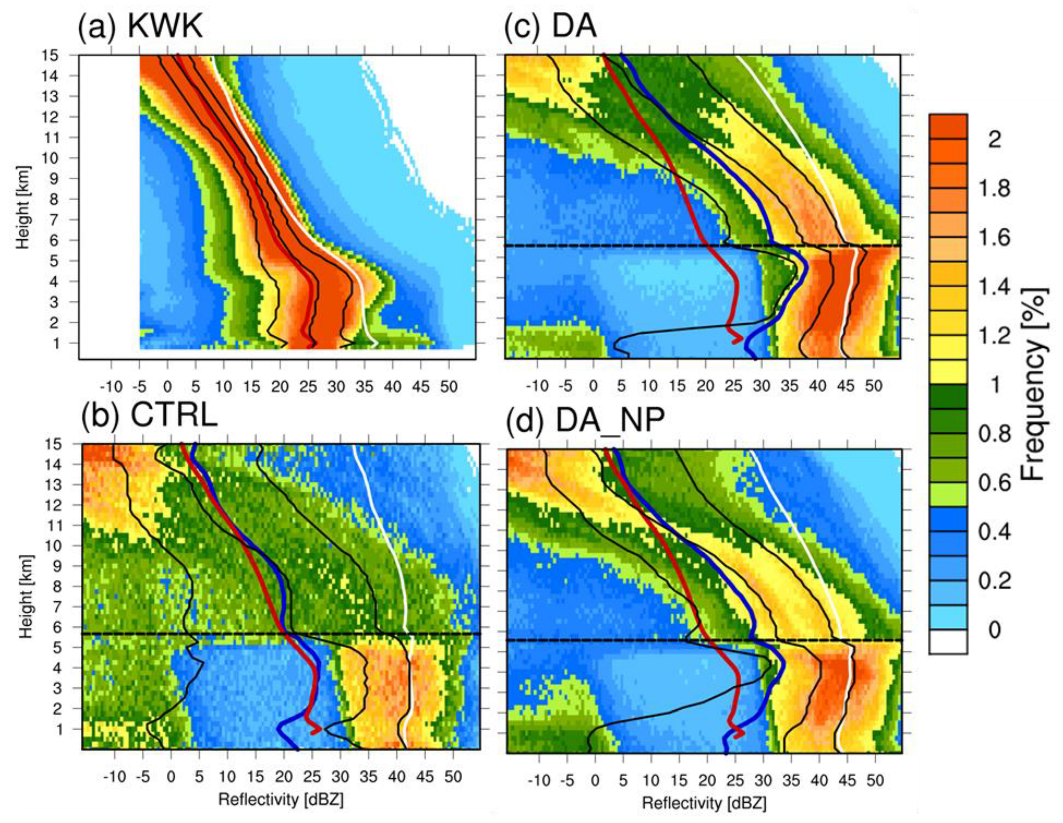
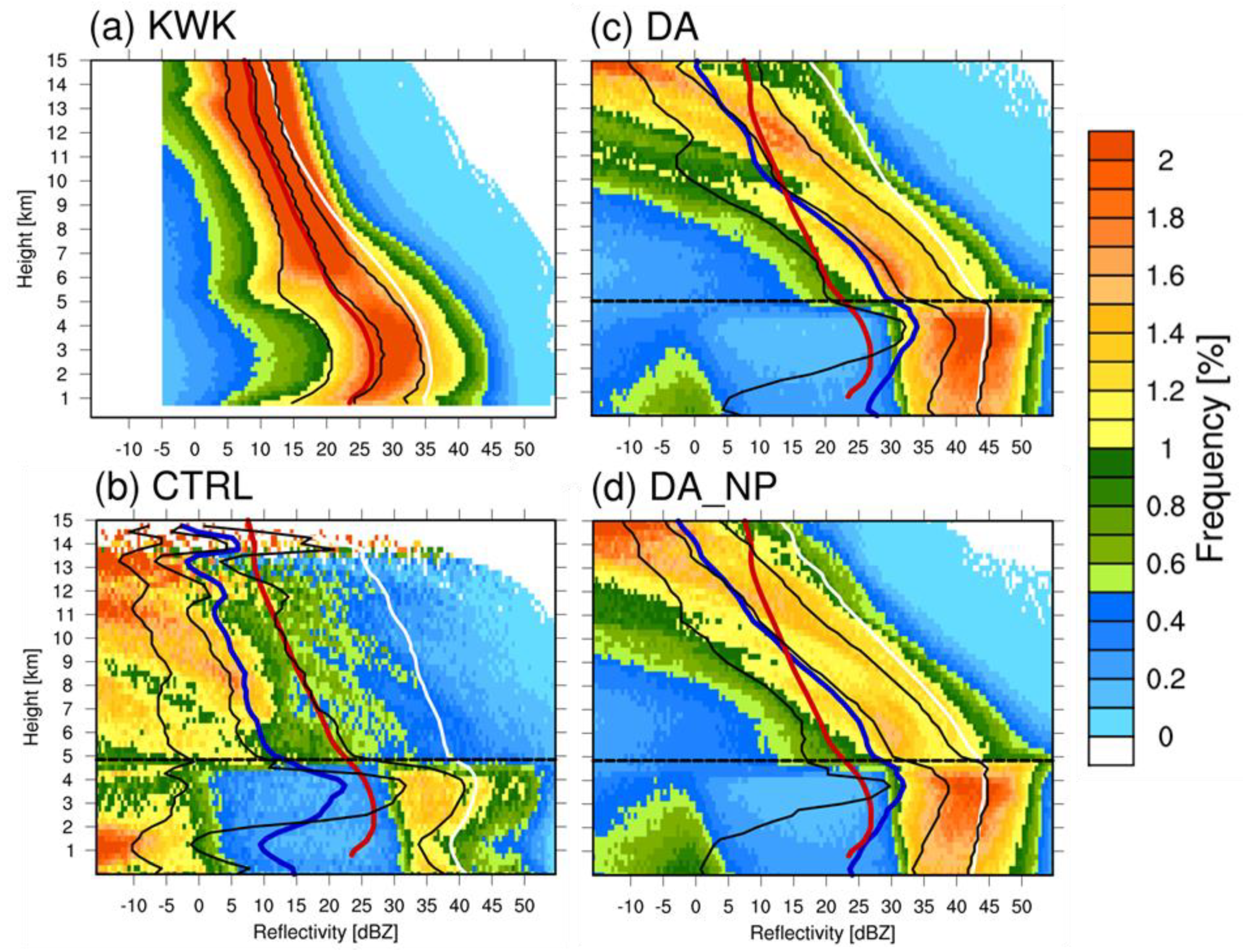
3.4. CFADs
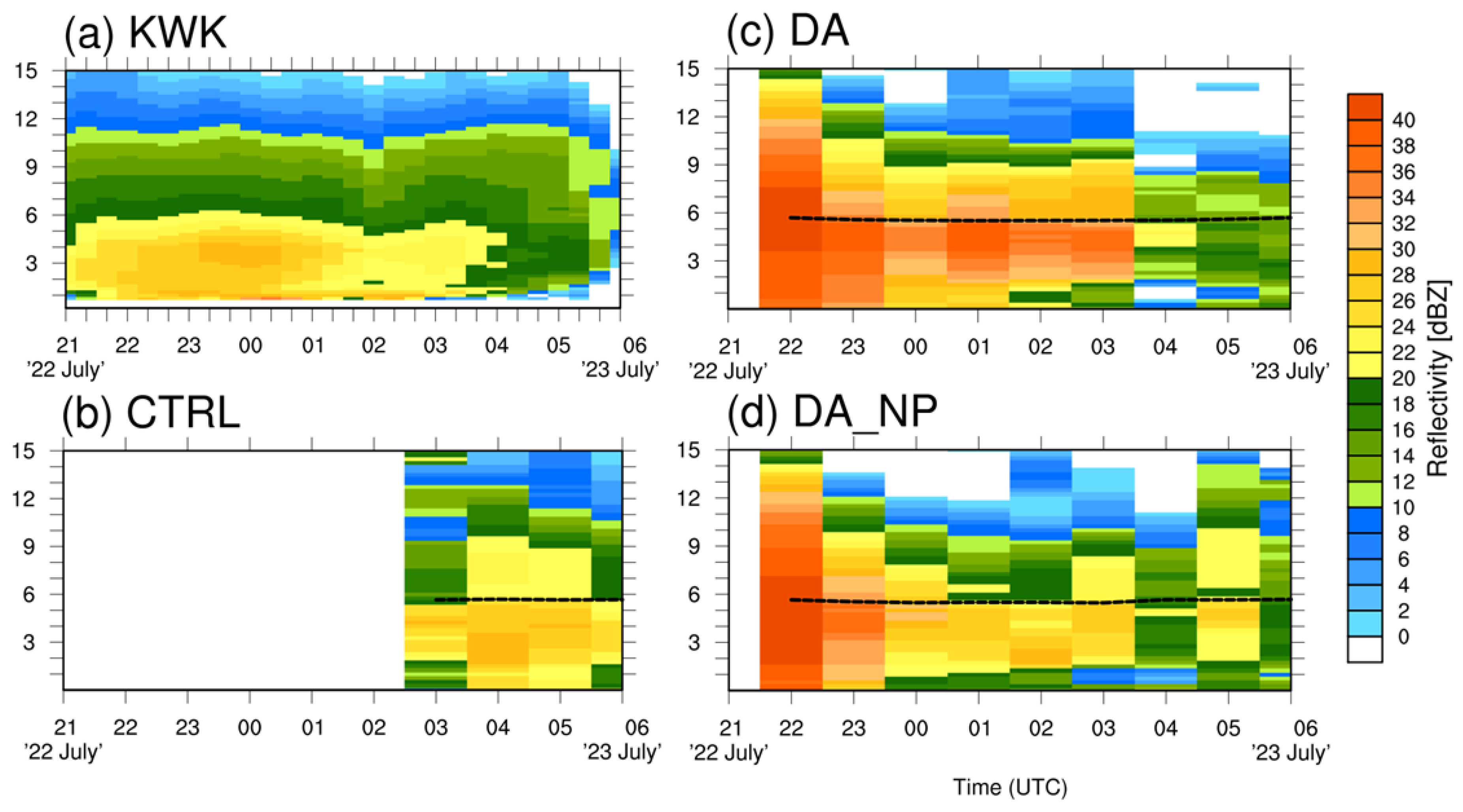
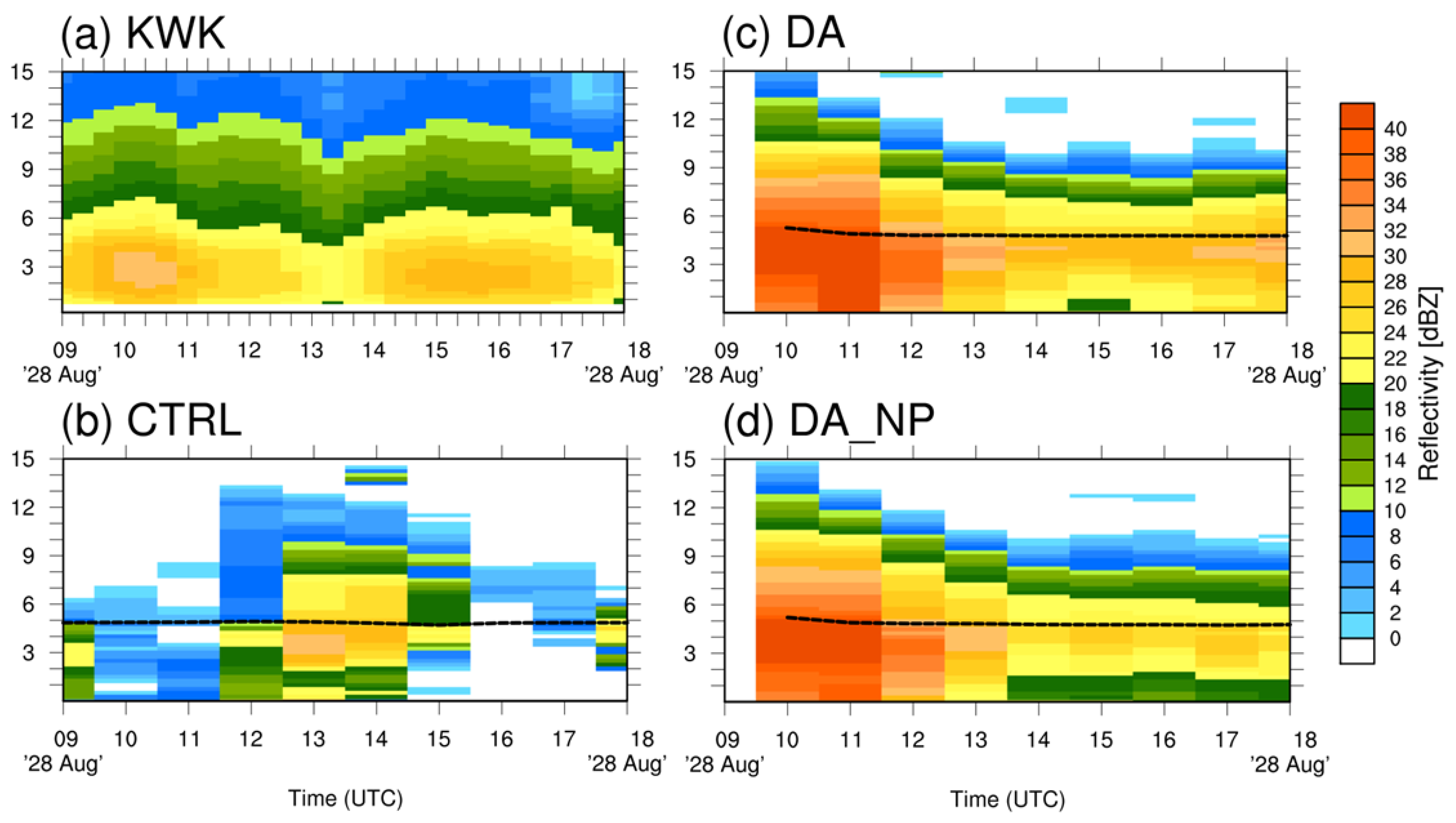
3.5. Time–Height Cross-Sections (THCS)
4. Summary and Conclusions
Author Contributions
Funding
Conflicts of Interest
References
- Korea Meteorological Society (KMS). Yealy KMA 2017 Wearther; KMA: Seoul, Korea, 2018; p. 10. [Google Scholar]
- Orlanski, I. A rational subdivision of scales for atmospheric processes. Bull. Am. Meteorol. Soc. 1975, 56, 527–530. [Google Scholar]
- Anthes, R.A.; Kuo, Y.H.; Baumhefner, D.P.; Errico, R.M.; Bettge, T.W. Predictability of Mesoscale Atmospheric Motions. Adv. Geophys. 1985, 28, 159–202. [Google Scholar]
- Lim, S.; Allabakash, S.; Chandrasekar, V.; Min, K.-H.; Choo, J.; Jang, B. X-Band Dual-Polarization Radar Observations of Snow Growth Processes of a Severe Winter Storm: Case of 12 December 2013 in South Korea. J. Atmos. Ocean. Technol. 2019, 36, 1217–1235. [Google Scholar] [CrossRef]
- Albers, S.C.; McGinley, J.A.; Birkenheuer, D.L.; Smart, J.R. The Local Analysis and Prediction System (LAPS): Analyses of Clouds, Precipitation, and Temperature. Weather Forecast. 1996, 11, 273–287. [Google Scholar] [CrossRef] [Green Version]
- Souto, M.J.; Balseiro, C.F.; Pérez-Muñuzuri, V.; Xue, M.; Brewster, K. Impact of Cloud Analysis on Numerical Weather Prediction in the Galician Region of Spain. J. Appl. Meteorol. 2003, 42, 129–140. [Google Scholar] [CrossRef] [Green Version]
- Gao, J.; Stensrud, D.J. Assimilation of reflectivity data in a convective-scale, cycled 3DVAR framework with hydrometeor classification. J. Atmos. Sci. 2012, 69, 1054–1065. [Google Scholar] [CrossRef]
- Wang, H.; Sun, J.; Fan, S.; Huang, X.-Y. Indirect assimilation of radar reflectivity with WRF 3D-Var and its impact on prediction of four summertime convective events. J. Appl. Meteorol. Climatol. 2013, 52, 889–902. [Google Scholar] [CrossRef]
- Gao, S.; Min, J.; Liu, L.; Ren, C. The development of a hybrid EnSRF-En3DVar system for convective-scale data assimilation. Atmos. Res. 2019, 229, 208–223. [Google Scholar] [CrossRef]
- Lee, Y.-H.; Min, K.-H. High-resolution modeling study of an isolated convective storm over Seoul Metropolitan area. Meteorol. Atmos. Phys. 2019, in press. [Google Scholar] [CrossRef]
- Abhilash, S.; Sahai, A.; Mohankumar, K.; George, J.P.; Das, S. Assimilation of Doppler weather radar radial velocity and reflectivity observations in WRF-3DVAR system for short-range forecasting of convective storms. Pure Appl. Geophys. 2012, 169, 2047–2070. [Google Scholar] [CrossRef]
- Bachmann, K.; Keil, C.; Craig, G.; Weissmann, M.; Welzbacher, C. Predictability of deep convection in idealized and operational forecasts: Effects of radar data assimilation, orography and synoptic weather regime. Mon. Weather Rev. 2019, in press. [Google Scholar] [CrossRef]
- Gao, J.; Fu, C.; Kain, J.; Stensrud, D.J. OSSEs for an ensemble 3DVAR data assimilation system with radar observations of convective storms. J. Atmos. Sci. 2016, 73, 2403–2426. [Google Scholar] [CrossRef]
- Hu, M.; Xue, M.; Gao, J.; Brewster, K. 3DVAR and Cloud Analysis with WSR-88D Level-II Data for the Prediction of the Fort Worth, Texas, Tornadic Thunderstorms. Part II: Impact of Radial Velocity Analysis via 3DVAR. Mon. Weather Rev. 2006, 134, 699–721. [Google Scholar] [CrossRef]
- Sugimoto, S.; Crook, N.A.; Sun, J.; Xiao, Q.; Barker, D.M. An examination of WRF 3DVAR radar data assimilation on its capability in retrieving unobserved variables and forecasting precipitation through observing system simulation experiments. Mon. Weather Rev. 2009, 137, 4011–4029. [Google Scholar] [CrossRef]
- Sun, J.; Wang, H. Radar Data Assimilation with WRF 4D-Var. Part II: Comparison with 3D-Var for a Squall Line over the U.S. Great Plains. Mon. Weather Rev. 2013, 141, 2245–2264. [Google Scholar] [CrossRef]
- Xiao, Q.; Sun, J. Multiple-radar data assimilation and short-range quantitative precipitation forecasting of a squall line observed during IHOP_2002. Mon. Weather Rev. 2007, 135, 3381–3404. [Google Scholar] [CrossRef]
- Xiao, Q.; Kuo, Y.-H.; Sun, J.; Lee, W.-C.; Barker, D.M.; Lim, E. An approach of radar reflectivity data assimilation and its assessment with the inland QPF of Typhoon Rusa (2002) at landfall. J. Appl. Meteorol. Climatol. 2007, 46, 14–22. [Google Scholar] [CrossRef] [Green Version]
- Wattrelot, E.; Caumont, O.; Mahfouf, J.-F. Operational Implementation of the 1D+3D-Var Assimilation Method of Radar Reflectivity Data in the AROME Model. Mon. Weather Rev. 2014, 142, 1852–1873. [Google Scholar] [CrossRef] [Green Version]
- Min, K.-H.; Kim, Y.-H. Assimilation of null-echo from radar data for QPF. In Proceedings of the 17th WRF Users’ Workshop, Boulder, CO, USA, 27 June–1 July 2016. [Google Scholar]
- Gao, S.; Sun, J.; Min, J.; Zhang, Y.; Ying, Z. A scheme to assimilate “no rain” observations from Doppler radar. Weather Forecast. 2018, 33, 71–88. [Google Scholar] [CrossRef]
- Xiao, Q.; Kuo, Y.-H.; Sun, J.; Lee, W.-C.; Lim, E.; Guo, Y.-R.; Barker, D.M. Assimilation of Doppler radar observations with a regional 3DVAR system: Impact of Doppler velocities on forecasts of a heavy rainfall case. J. Appl. Meteorol. 2005, 44, 768–788. [Google Scholar] [CrossRef]
- Ye, B.-Y.; Lee, G.; Park, H.-M. Identification and removal of non-meteorological echoes in dual-polarization radar data based on a fuzzy logic algorithm. Adv. Atmos. Sci. 2015, 32, 1217–1230. [Google Scholar] [CrossRef]
- Barker, D.M.; Huang, W.; Guo, Y.-R.; Bourgeois, A.J.; Xiao, Q.N. A three-dimensional variational data assimilation system for MM5: Implementation and initial results. Mon. Weather Rev. 2004, 132, 897–914. [Google Scholar] [CrossRef] [Green Version]
- Barker, D.M.; Coauthors. The Weather Research and Forecasting (WRF) Model’s Community Variational/Ensemble Data Assimilation System: WRFDA. Bull. Am. Meteorol. Soc. 2012, 93, 831–843. [Google Scholar] [CrossRef] [Green Version]
- Parrish, D.F.; Derber, J.C. The National Meteorological Center’s spectral statistical-interpolation analysis system. Mon. Weather Rev. 1992, 120, 1747–1763. [Google Scholar] [CrossRef]
- Lin, Y.; Farley, R.D.; Orville, H.D. Bulk paramete-rization of the snow field in a cloud model. J. Clim. Appl. Meteorol. 1983, 22, 1065–1092. [Google Scholar] [CrossRef] [Green Version]
- Gilmore, M.S.; Wicker, L.J. The influence of mid-tropospheric dryness on supercell morphology and evo-lution. Mon. Weather Rev. 1998, 126, 943–958. [Google Scholar] [CrossRef]
- Dowell, D.C.; Wicker, L.J.; Snyder, C. Ensemble Kalman filter assimilation of radar observations of the 8 May 2003 Oklahoma City supercell: Influences of refl-ectivity observations on storm-scale analyses. Mon. Weather Rev. 2011, 139, 272–294. [Google Scholar] [CrossRef] [Green Version]
- Smith, P.L., Jr.; Myers, C.G.; Orville, H.D. Radar reflectivity factor calculations in numerical cloud models using bulk parameterization of precipitation processes. J. Appl. Meteorol. 1975, 14, 1156–1165. [Google Scholar] [CrossRef] [Green Version]
- Sun, J.; Crook, N.A. Dynamical and microphysical retrieval from Doppler radar observations using a cloud model and its adjoint. Part I: Model development and simulated data experiments. J. Atmos. Sci. 1997, 54, 1642–1661. [Google Scholar] [CrossRef]
- Skamarock, W.C.; Klemp, J.B.; Dudhia, J.; Gill, D.O.; Barker, D.M.; Wang, W.; Powers, J.G. A Description of the Advanced Research WRF Version 2. NCAR Tech. Note NCAR/TN-4681STR; UCAR Communications: Boulder, CO, USA, 2008; 88p. [Google Scholar] [CrossRef] [Green Version]
- Zheng, Y.; Alapaty, K.; Herwehe, J.S.; Del Genio, A.; Niyogi, D. Improving high-resolution weather forecasts using the Weather Research and Forecasting (WRF) Model with an updated Kain–Fritsch scheme. Mon. Weather Rev. 2016, 144, 833–860. [Google Scholar] [CrossRef]
- Lim, K.-S.S.; Hong, S.-Y. Development of an effective double-moment cloud microphysics scheme with prognostic cloud condensation nuclei (CCN) for weather and climate models. Mon. Weather Rev. 2010, 138, 1587–1612. [Google Scholar] [CrossRef] [Green Version]
- Hong, S.-Y.; Noh, Y.; Dudhia, J. A new vertical diffusion package with an explicit treatment of entrainm-ent processes. Mon. Weather Rev. 2006, 134, 2318–2341. [Google Scholar] [CrossRef] [Green Version]
- Mlawer, E.J.; Taubman, S.J.; Brown, P.D.; Iacono, M.J.; Clough, S.A. Radiative transfer for inhomogeneous atmospheres: RRTM, a validated correlated-k model for the longwave. J. Geophys. Res. 1997, 102, 16663–16682. [Google Scholar] [CrossRef] [Green Version]
- Dudhia, J. Numerical study of convection observed during the Winter Monsoon Experiment using a mesosca-le two-dimensional model. J. Atmos. Sci. 1989, 46, 3077–3107. [Google Scholar] [CrossRef]
- Jimenez, P.A.; Dudhia, J.; Gonzalez-Rouco, J.F.; Navarro, J.; Montavez, J.P.; Garcia-Bustamante, E. A revi-sed scheme for the WRF surface layer formulation. Mon. Weather Rev. 2012, 140, 898–918. [Google Scholar] [CrossRef] [Green Version]
- Tewari, M.; Chen, F.; Wang, W.; Dudhia, J.; LeMone, M.A.; Mitchell, K.; Ek, M.; Gayno, G.; Wegiel, J.; Cuenca, R.H. Implementation and verification of the unified Noah land-surface model in the WRF Model. In Proceedings of the 20th Conference on Weather Analysis and Forecasting, Seattle, WA, USA, 10–15 January 2004; p. 14.2a. [Google Scholar]
- Yuter, S.E.; Houze, R.A. Three-dimensional kinematic and microphysical evolution of Florida cumulonimbus. Part II: Frequency distributions of vertical velocity, reflectivity, and differential reflectivity. Mon. Weather Rev. 1995, 123, 1941–1963. [Google Scholar] [CrossRef]
- Wang, J.-J.; Carey, L. The Development and Structure of an Oceanic Squall-Line System during the South China Sea Monsoon Experiment. Mon. Weather Rev. 2005, 133, 1544–1561. [Google Scholar] [CrossRef]
- Min, K.-H.; Choo, S.-H.; Lee, D.-H.; Lee, G.-W. Evaluation of WRF Cloud Microphysics Schemes Using Radar Observations. Weather Forecast. 2015, 30, 1571–1589. [Google Scholar] [CrossRef]
- Cecil, D.J. Relating passive 37-GHz scattering to radar profiles in strong convection. J. Appl. Meteorol. Climatol. 2011, 50, 233–240. [Google Scholar] [CrossRef]


| Purpose | Observations | Variables | Horizontal Resolution | Vertical Resolution | Time Period | Time Resolution |
|---|---|---|---|---|---|---|
| Data assimilation | Radar | Reflectivity (dBZ), Doppler radial velocity (m·s−1) | 1, 3 km * | 200 m | 3 h | 30 min |
| AWS | Surface pressure (hPa), sea level pressure (hPa), 10-min average wind speed (m·s−1) and direction (°), temperature and dew point temperature (K) | - | ||||
| Verification | Precipitation (mm) | 1 km * | - | 9 h | 1 h | |
| Radiosonde | Water vapor mixing ratio (g·kg−1), temperature (K), wind speed (m·s−1) and direction (°) | Point | 50 hPa | 0000 or 1200 UTC * | ||
| D01 | D02 | D03 | |
|---|---|---|---|
| Resolution | 9 km | 3 km | 1 km |
| Number of Grids | 240 × 240 × 60 | 151 × 151 × 60 | 226 × 196 × 60 |
| Cumulus | Multiscale Kain–Fritsch scheme | ||
| Microphysics | WRF Double Moment 6 class scheme | ||
| Planetary Boundary Layer | Yonsei University Scheme | ||
| Surface Layer | Revised MM5 Monin–Obukhov scheme | ||
| Land Surface | Unified Noah land surface model | ||
| Long-Wave Radiation | Rapid radiative transfer model scheme | ||
| Short-Wave Radiation | Dudhia scheme | ||
| Initial and Boundary Conditions | National Center for Environmental Prediction Global Forecast System 0.25 Degree Historical Archive | ||
| Assimilated Observation Data | |
|---|---|
| CTRL | No data assimilation |
| DA | AWS + radar radial velocity + radar reflectivity |
| DA_NP | AWS + radar radial velocity + radar reflectivity + null echoes |
| Forecast Period | Total Cumulative Precipitation (mm) | Maximum Rain Rate (mm·h−1) | Maximum CAPE * (J·kg−1) | ||
|---|---|---|---|---|---|
| CTRL | DA and DA_NP | ||||
| Case 1 | 2017.07.02.0600 UTC ~ 1800 UTC | 2017.07.02.0900 UTC ~ 1800 UTC | 55 | 55.0 | 1233 |
| Case 2 | 2017.07.22.1800 UTC ~ 2017.07.23.0600 UTC | 2017.07.22.2100 UTC ~ 2017.07.23.0600 UTC | 110 | 67.0 | 1521 |
| Case 3 | 2018.08.28.0600 UTC ~ 1800 UTC | 2018.08.28.0900 UTC ~ 1800 UTC | 180 | 73.0 | 1468 |
| Observation | Total | |||
|---|---|---|---|---|
| Yes | No | |||
| Forecast | Yes | Hits = A | False alarms = B | Forecast Yes |
| No | Misses = C | Correct negative = D | Forecast No | |
| Total | Observed Yes | Observed No | Total = N | |
| Experiment | Bias (mm) | MAE (mm) | RMSE (mm) | |
|---|---|---|---|---|
| Case 1 | CTRL | −15.3 | 19.2 | 28.6 |
| DA | −9.1 | 20.0 | 30.0 | |
| DA_NP | −8.8 | 18.2 | 26.7 | |
| Case 2 | CTRL | −31.4 | 34.0 | 47.3 |
| DA | 12.1 | 28.8 | 40.0 | |
| DA_NP | 2.3 | 21.3 | 31.4 | |
| Case 3 | CTRL | −48.5 | 48.7 | 62.7 |
| DA | 17.5 | 31.2 | 43.6 | |
| DA_NP | 2.8 | 23.3 | 35.4 | |
| Average | CTRL | −31.7 | 34.0 | 46.2 |
| DA | 6.9 | 26.7 | 37.9 | |
| DA_NP | −1.2 | 20.9 | 31.2 |
© 2020 by the authors. Licensee MDPI, Basel, Switzerland. This article is an open access article distributed under the terms and conditions of the Creative Commons Attribution (CC BY) license (http://creativecommons.org/licenses/by/4.0/).
Share and Cite
Lee, J.-W.; Min, K.-H.; Lee, Y.-H.; Lee, G. X-Net-Based Radar Data Assimilation Study over the Seoul Metropolitan Area. Remote Sens. 2020, 12, 893. https://doi.org/10.3390/rs12050893
Lee J-W, Min K-H, Lee Y-H, Lee G. X-Net-Based Radar Data Assimilation Study over the Seoul Metropolitan Area. Remote Sensing. 2020; 12(5):893. https://doi.org/10.3390/rs12050893
Chicago/Turabian StyleLee, Ji-Won, Ki-Hong Min, Young-Hee Lee, and GyuWon Lee. 2020. "X-Net-Based Radar Data Assimilation Study over the Seoul Metropolitan Area" Remote Sensing 12, no. 5: 893. https://doi.org/10.3390/rs12050893
APA StyleLee, J.-W., Min, K.-H., Lee, Y.-H., & Lee, G. (2020). X-Net-Based Radar Data Assimilation Study over the Seoul Metropolitan Area. Remote Sensing, 12(5), 893. https://doi.org/10.3390/rs12050893