Mapping Forest Canopy Fuels in the Western United States with LiDAR–Landsat Covariance

Abstract

Comprehensive spatial coverage of forest canopy fuels is relied upon by fire management in the US to predict fire behavior, assess risk, and plan forest treatments. Here, a collection of light detection and ranging (LiDAR) datasets from the western US are fused with Landsat-derived spectral indices to map the canopy fuel attributes needed for wildfire predictions: canopy cover (CC), canopy height (CH), canopy base height (CBH), and canopy bulk density (CBD). A single, gradient boosting machine (GBM) model using data from all landscapes is able to characterize these relationships with only small reductions in model performance (mean 0.04 reduction in R²) compared to local GBM models trained on individual landscapes. Model evaluations on independent LiDAR datasets show the single global model outperforming local models (mean 0.24 increase in R²), indicating improved model generality. The global GBM model significantly improves performance over existing LANDFIRE canopy fuels data products (R² ranging from 0.15 to 0.61 vs. −3.94 to −0.374). The ability to automatically update canopy fuels following wildfire disturbance is also evaluated, and results show intuitive reductions in canopy fuels for high and moderate fire severity classes and little to no change for unburned to low fire severity classes. Improved canopy fuel mapping and the ability to apply the same predictive model on an annual basis enhances forest, fuel, and fire management.

1. Introduction

Characterization of forest structure remains a priority for a variety of scientific research and land management objectives [1,2,3,4,5,6]. Forest management across the Earth now relies on spatial data derived from remote sensing to inform policy and decision making [7]. For example, the LANDFIRE project produces nationally consistent and comprehensive forest canopy fuel maps for the US from Landsat satellite imagery and facilitates landscape-scale management including fuel and restoration treatment planning and assessment [8,9,10,11], prescribed fire planning and implementation [12], and wildfire prediction, suppression, impact mitigation, rehabilitation, and assessment [10,13,14,15].

For wildfire management in particular, LANDFIRE provides the spatial data for fire models that predict the spread and intensity of wildfires [16]. These predictions are essential for wildfire risk assessments, which are increasing in necessity because strategic and tactical fire management decisions are now called to be explicitly risk based [14,17]. Wildfires are increasing in size and severity with unprecedented destruction and associated costs [18,19,20]. Climate change is set to increase aridity across the western US with expected increases to fire disturbance [21,22]. Accurate, up-to-date, and comprehensive datasets are thus needed for effective fire management and could prevent loss of life and property and promote ecosystem health.

To create these broad spatial data, standard approaches utilize field measurements, which provide explicit measurements of attributes [23]. These are then related to satellite imagery thereby creating spatially-complete datasets [24]. Such assessments have risen in scale from local [25] to regional [26] and global assessments [27] in parallel with the rise in image availability, computing performance, and analytical sophistication. However, traditional field-based approaches are often labor intensive, do not capture the range of variation on the landscape, have inconsistent data collection methods, and cannot feasibly capture many sought-after three-dimensional (3D) attributes [28,29].

Light detection and ranging (LiDAR), a now pervasive active remote sensing technology, combined with a scanning system (airborne laser scanner (ALS)), has provided large-area 3D datasets and facilitated the conceptualization of new forest attributes and statistical relationships to established forest metrics [30,31]. Field data have been crucial to the development of these attributes, but the consistency and accuracy of LiDAR allows the application of statistical relationships for forest attribute prediction over a diversity of geographic areas and reasonably similar forest types [32,33]. However, the spatial and temporal scales of these LiDAR data and existing predictive models are still limited for a variety of management needs. LiDAR data are often incomplete, out-of-date, or not available, and predictive models derived from these data are often overfit to specific landscapes and forest types [33].

As satellite imagery provides the necessary spatial and temporal coverage and LiDAR provides accurate 3D characterization, many studies have harnessed their complementary strengths and fused them to create comprehensive spatial datasets [34]. LiDAR metrics have been used directly as the response variable (e.g., canopy cover and height) or indirectly as the predictor variable of a modeled response (e.g., biomass, basal area, and Lorey’s height). Correlations of satellite imagery to basic attributes characterizing vegetation coverage fractions, such as forest canopy cover, are well documented, especially from the series of Landsat satellites [35], but the ability of satellite imagery to characterize complex forest attributes, such as canopy height and height variability [36,37,38,39,40,41,42], basal area [43], biomass [34,44,45,46], and other measures of structural complexity [47,48,49] has come relatively recently and are aided by LiDAR data. Though the potential for these types of characterizations using imagery has been exploited for several decades [50], the ubiquity of LiDAR datasets with large numbers of samples and accurate 3D characterizations have enabled more robust assessments over broad areas [49].

Canopy cover (CC) and canopy height (CH) can be directly measured by LiDAR while canopy bulk density (CBD) can be estimated using regression equations utilizing LiDAR-derived CH and CC as predictor variables [51,52]. Andersen et al. [53] developed multi-variate models to estimate canopy fuel parameters specific to the Pacific Northwest region of the US and Peterson et al. [52] adopted generalized canopy base height (CBH) and CBD conceptualizations. For CBH, many formulations exist including using LiDAR metrics as direct surrogates. For example, 1st percentile LiDAR heights [54], 25th percentile LiDAR height [55], and one standard deviation (SD) of LiDAR heights subtracted from mean LiDAR height [52,56]. These LiDAR-based estimates of CBH and CBD capture the spatial variation in 3D canopy structure important for fire modeling. While different in their conception from field-based estimates, the absolute values of these variables are not as important as representing the structural variability across the landscape because fire behavior modelers often need to calibrate canopy fuel values to match observed fire behavior to fire model outputs [9,57].

In conjunction with LiDAR-based training data, the rise of machine learning techniques has also contributed to the increase in correlative and predictive power for remote sensing [58]. Mousivand et al. [59] showed that the sum of second-order interactions was greater than first-order canopy effects on spectral reflectance at the scales and wavelengths of Landsat imagery. Machine learning algorithms have the ability to characterize these complex relationships given appropriate training data. Gradient boosting machines (GBMs) are one of these algorithms now applied in remote sensing and ecological sciences [60]. They combine the advantages of tree-based algorithms with a boosting approach that adaptively combines many simple regression trees [61,62].

Predictive models capable of reasonable accuracy across a diversity of landscapes have been a research priority for remote sensing and forestry applications [32,33,46]. The inability of models derived from localized datasets to apply to other landscapes stems from three primary and related issues: model overfitting [33,63], mis-specified predictor variables not fully characterizing the response, and spatial and temporal variance in the feature–response relationships—in this case, the LiDAR–Landsat relationships [49]. These issues are compounded when integrating collections of ALS datasets acquired from different time periods and locations.

This study aims to address these issues while developing methods to produce comprehensive and accurate canopy fuels maps for the western US. Model overfitting is a common issue for algorithms such as GBMs [60,64]. Several strategies have been developed to increase model generality. These regularization techniques include hyperparameter tuning [65], which varies model parameters and utilizes a stopping metric to reduce overfitting. Sample weighting or balancing is also an important regularization technique [66,67] given the arbitrary spatial and temporal extents of ALS datasets. Forest landscapes can have sample distributions that are heavily skewed or have high kurtosis in one or more canopy variables, which can bias model predictions. For large-area predictions, spatial and temporal variance in the LiDAR–Landsat relationships also leads to poor model performance if there is inadequate training data [32,46,68]. One solution is to create many localized models from each individual LiDAR dataset and stitch the predictions together. However, determining boundaries where each local model is most applicable would be difficult. Conversely, a single global model can be used with either sufficient generality or including locational predictor variables to correct for spatial variance [47,49]. A select set of models, each trained on biophysically stratified data, may represent a compromise between these two extremes.

In this study, canopy fuels are estimated from LiDAR datasets and used as training data for GBM models using Landsat spectral data for predictor variables. Model predictions are then compared to current LANDFIRE data to quantify improvements due to LiDAR training data, GBM modeling, and regularization techniques. The research has three objectives:

(1)

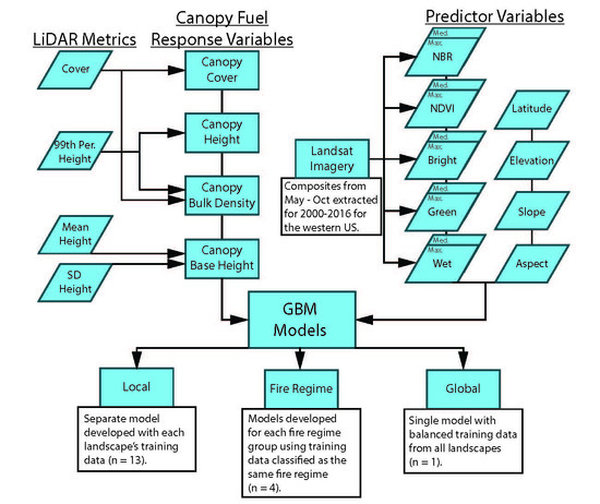
Create and compare local, biophysically stratified, and global predictive model(s) of canopy fuels variables than can be applied to forested areas in the western US;

(2)

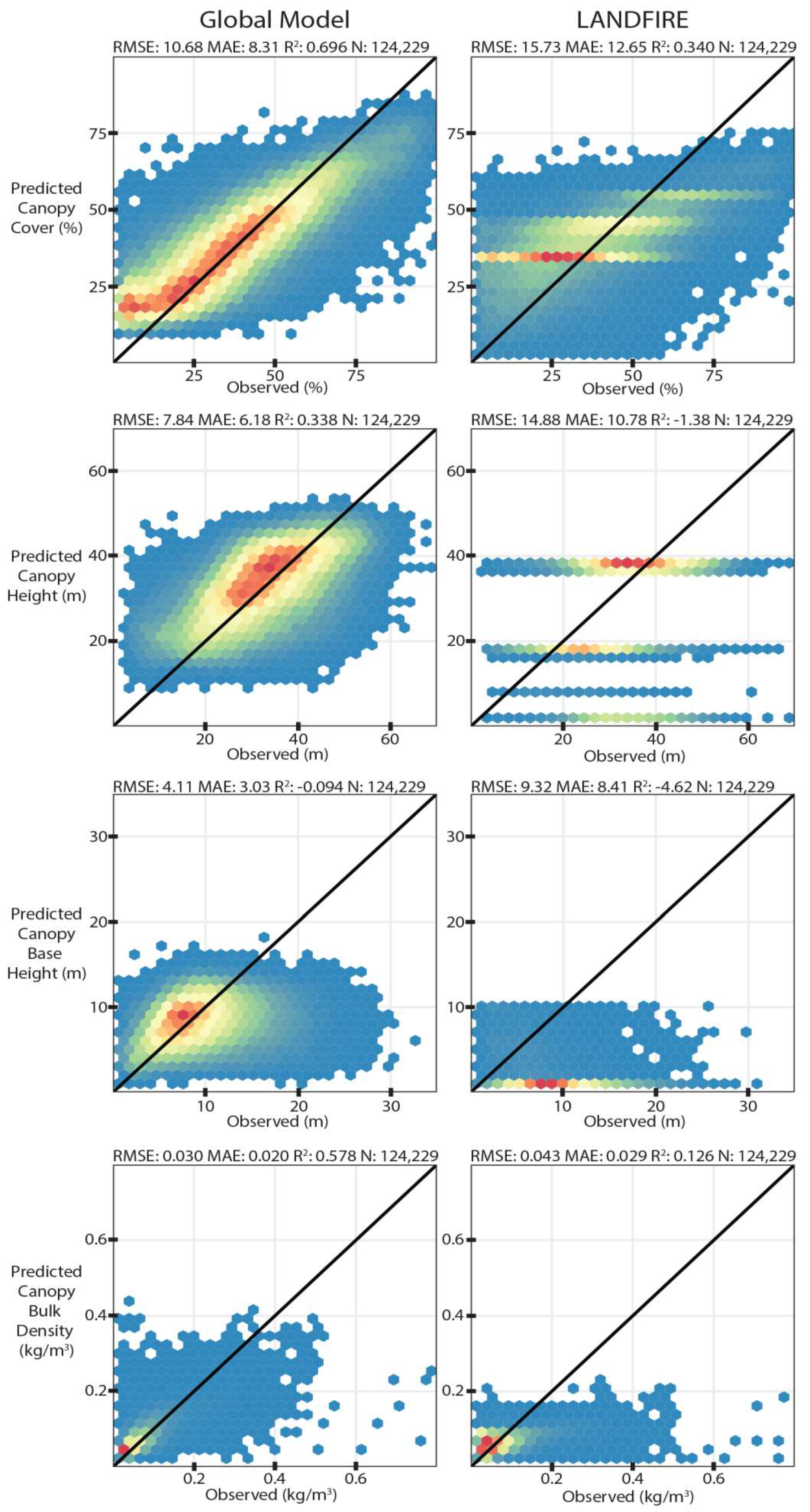
Compare model predictions to current LANDFIRE products;

(3)

Assess selected model(s) ability to update canopy layers following wildfire disturbance.

2. Materials and Methods

2.1. Data

LiDAR datasets were selected based on availability and to represent the diversity of conifer forests, climates, and disturbance regimes in the western contiguous US (Figure 1). LiDAR acquisitions were ultimately grouped into sixteen landscapes for analysis based on proximity and vegetation similarities. Hereafter, each set of grouped LiDAR acquisitions is referred to as a landscape dataset. Thirteen landscapes were used for model training, validation, and testing (training landscapes), while three landscapes were used exclusively for model testing (test landscapes). All LiDAR data acquisition parameters followed, at a minimum, the requirements for the US Geological Survey’s Quality Level 1 [69]. Important collection parameters include ≥ 3 returns/pulse, ≥ 8 returns/m², and a relative vertical accuracy ≤ 0.06 m root-mean-square deviation (RMSD). LiDAR data totaled 1,258,993 ha for training and validation and 265,225 ha for testing. Landscape elevations range from 0 to 3599 m a.s.l. and precipitation normals range from less than 200 mm to over 4000 mm annually [70]. At least one dataset is within each EPA Level I forest ecoregion of the western US (Figure 1).

2.2. LiDAR Processing

LiDAR point clouds were processed through FUSION software [71] to extract height above ground and calculate metrics to match the 30 m Landsat cell resolution. All subsequent analyses were conducted at the 30 m cell resolution.

Table 1. Summary of canopy fuel response variables (LiDAR-sourced) and predictor variables used in the study. Existing vegetation type (EVT) and fire regime group (FRG) LANDFIRE variables filtered data instead of being used as predictor variables for model development. Median and maximum Landsat indices derived from May to Oct imagery.

Source	Variable Name	Description	Citations
LiDAR	Canopy Cover (CC) (%)	Percentage of first returns above 2 m	[52,72,73]
	Canopy Height (CH) (m)	99th percentile return height	[52]
	Canopy Base Height (CBH) (m)	Mean return height minus standard deviation of heights	[52,56]
	Canopy Bulk Density (CBD) (kg/m3)	$\begin{array}{ll}e^(-2.489+0.034& \left(CC\right)-0.357\left(SH1\right)\\ & -0.601\left(SH2\right)-1.107\left(PJ\right)\\ & -0.001\left(CC\ast SH1\right)\\ & -0.002\left(CC\ast SH2\right))\end{array}$ If CH is 0–15 m: stand height class (SH), SH1 = 0 and SH2 = 0 If CH is 15–30 m: SH1 = 1 and SH2 = 0 If CH is 30–91 m: SH1 = 0 and SH2 = 1 If EVT equals Pinyon or Juniper type: PJ = 1 else PJ = 0	[51]
Landsat	Med NDVI	Median normalized difference vegetation index (NDVI) value	[74]
	Max NDVI	Maximum NDVI value	[74]
	Med NBR	Median normalized burn ratio (NBR)	[75]
	Max NBR	Maximum NBR	[75]
	Med Bright	Median tasseled cap brightness	[76,77,78]
	Max Bright	Maximum tasseled cap brightness	[76,77,78]
	Med Green	Median tasseled cap greenness	[76,77,78]
	Max Green	Maximum tasseled cap greenness	[76,77,78]
	Med Wet	Median tasseled cap wetness	[76,77,78]
	Max Wet	Maximum tasseled cap wetness	[76,77,78]
LANDFIRE	EVT	Existing vegetation type	[16]
	FRG	Fire regime group	[79]
	Slope (%)	Slope
	Aspect (deg)	Aspect
	Elev (m)	Elevation
	Lat (deg)	Latitude

shows the formulation of the canopy fuel metrics from LiDAR. CH, CC, and CBH are defined directly from the LiDAR metrics. For CBH and CBD estimation, multiple possible formulations exist [52], and we chose parsimonious definitions that could apply to many forest types in the western US. For CBH, LiDAR mean height of canopy points minus one standard deviation of heights provided a characterization with adequate correlation to field-based estimates at multiple study sites (R² = 0.547) [52]. For CBD, we used an established equation derived from field data and inserted LiDAR-derived CH and CC values [51,52]. LiDAR data were filtered for a minimum canopy height of 2 m, canopy cover of 2%, and the LANDFIRE existing vegetation type (EVT) classified as a forest type to ensure that non-forested pixels did not contaminate samples.

2.3. Landsat and LANDFIRE Data Processing

Landsat indices (Table 1) were calculated for the contiguous US for the period of 2000–2016 using May to October imagery at an annual timestep. Median and maximum values of each index for each year were calculated using US Geological Survey Landsat 5 TM, Landsat 7 ETM+, and Landsat 8 OLI surface reflectance products created using the Landsat Ecosystem Disturbance Adaptive Processing (LEDAPS) algorithm [80,81]. The use of both median and maximum values followed studies, such as Egorov et al. [82], that showed multi-temporal metrics derived from annual composites enhanced predictive performance for forest canopy models and also followed the hypothesis that multi-temporal imagery can capture differences in shadowing (due to changing sun-angles) related to tree height [83]. Landsat TM and ETM+ were merged and constituted the data source for the period of 2000–2014, and OLI data was used for the period of 2015–2016. Equations for spectral calculations are within the citations in Table 1. Pixels were filtered for contamination by clouds, cloud shadows, and adjacency to clouds, snow, and water. All Landsat data was processed within Google Earth Engine, exported, and then mosaicked into multi-band rasters organized by year.

Topography and geographic metrics of slope, aspect, elevation, and latitude were taken from LANDFIRE [16]. Fire regime groups (FRGs) [79] and existing vegetation type (EVT) were also extracted along with LANDFIRE’s existing canopy fuel layers CC, CH, CBH, and CBD [51] for comparison to model outputs.

2.4. Dataset Stratification, Sample Weighting, and Model Development

All subsequent data processing and model development were completed using R statistical software in conjunction with the Apache Spark analytics engine. Spark is an open-source, parallel, scalable, and resilient Big Data processing environment [84]. H2O machine learning algorithms were employed within R and Spark using the R packages h2o [85], sparklyr [86], and rsparkling [87]. Data preprocessing, stratification, visualization, and weighting were completed using the R packages raster [88], ggplot2 [89], and dplyr [90].

Three data stratification approaches were devised, leading to three sets of models (Figure 2)—local models, models stratified by fire regime groups (FRGs), and a global model taking data from all landscapes. For the local models, training, validation, and test data were taken from within each individual landscape (Figure 1) and a separate model derived for each. Recognizing that these local models are likely overfit to their respective landscapes, they represent the baseline accuracy or maximum potential extractable information that subsequent, more generalized models can be compared to. Next, we hypothesized that the nature of the spectral relationships may vary across forest types and separate models stratified by a biophysical rationale may better characterize these relationships. Fire regime groups produced by LANDFIRE represent an integration of existing and potential vegetation, climate, topography, and disturbance regimes [79]. Forests within the same FRG classifications were expected to have similar structural and species assemblages and therefore more consistent spectral responses. For forested areas, four fire regime groups were present within the study area:

FRG 1: ≤ 35 year fire return interval, low and mixed severity;

FRG 3: 35–200 year fire return interval, low and mixed severity;

FRG 4: 35–200 year fire return interval, replacement severity;

FRG 5: > 200 year fire return interval, any severity.

FRG 5 represents a diverse category including multiple vegetation types across the US but in the western US and for the landscapes in this study, FRG 5 represents the western Cascade Mountains and coastal forests in the Mt. Baker, Hoh, North Coast, and South Coast landscapes. All pixels representing a particular FRG from all landscapes were binned and used to construct a model.

Finally, a global model containing all data from all landscapes was created as a parsimonious option requiring no stratification. However, with the significant differences in dataset sizes between landscapes (cf. Figure 1), predictor–response relationships in large datasets may dominate the smaller datasets. Thus, landscape datasets were randomly sampled so that each landscape’s contribution did not exceed 20% of the total sample size for the global model. This rule was also applied to the FRG models for the same purpose, but the proportion was adjusted to 30% for FRG 4 and FRG 5 because only a few landscapes contained enough data for training.

An additional sample weighting scheme was applied for every model to improve generality and the ability to characterize post-disturbance canopy fuels on any landscape. For each of the four canopy response variables (CC, CH, CBH, CBD), the range of values was assessed and then split into ten even-sized bins (e.g., CC: 1–10%, 11–20%, 21–30%, etc.). The bins were ordered by sample size, and the samples within the bin with the highest count all received a weighting value of one (i.e., would be considered once in the model). The other bin’s samples were then multiplied by the necessary weighting value so that the sum of the sample weights was equal across all bins. This effectively gave an equal weighting to the full range of values, helping to prevent model bias due to skewed or leptokurtic training data distributions. Several classes for certain models had very few samples within a class which led to extreme weighting values to few samples (> 100,000x weight in one case). Therefore, the maximum weight for any sample was set to 100x to reduce model instability created by extreme weighting.

Once stratification and weighting were completed, model development was then possible. From each model’s sample pool, 80% were selected for training, 10% for validation and internal error estimation for hyperparameter tuning, and 10% for testing and performance assessment. However, these testing data’s acquisition parameters, especially the year of acquisition, and the geographic location and vegetation type are still related to the particular landscape from which they were derived. Thus, three separate LiDAR datasets without any data used in the model training process were used as a final assessment of the local, FRG, and global model performance (Figure 1, red landscapes).

Table 2. Gradient boosting machine (GBM) model parameters. Those with multiple values were those utilized in the hyperparameter tuning process.

GBM Model Parameters	Value(s)
ntrees	Up to 4000
learn_rate	0.1
learn_rate_annealing	0.01
sample_rate	0.4, 0.6, 0.9, 1
col_sample_rate	0.6, 0.9, 1
col_sample_rate_per_tree	0.6, 0.9, 1
col_sample_rate_change_per_level	0.01, 0.9, 1.1
nbins	32, 64, 128, 256
min_split_improvement	0, 1 × 10−4, 1 × 10−6, 1 × 10−8
max_depth	20, 30, 40
histogram_type	AUTO, UniformAdaptive, QuantilesGlobal
stopping_metric	RMSE
stopping_tolerance	0.01
score_tree_interval	10
stopping_rounds	3

shows the GBM model parameters including those varied during hyperparameter tuning. For more explanation of each parameter see H2O.AI GBM documentation [91]. A maximum of ten models were trained before selecting each final model, and the various parameter options were randomly selected for each model run. Final model selection used minimum RMSE as the selection metric.

2.5. Spectral Response and Model Performance Assessment

In order to assess the variance in the relationships between the spectral predictor variables and the canopy fuel response variables, partial dependence plots were calculated for the local, FRG, and global models. Partial dependence plots assess the marginal effect of a single predictor variable on the response variable [62]. The major assumption is that the predictor variables are independent of each other. While the GBM model is resistant to multi-collinearity, if a predictor is highly correlated with another, then data combinations created from the predictor distributions can be highly unlikely in reality and result in biased partial dependence estimates. Thus, local, FRG, and global models were first trained on a reduced subset of predictor variables for creation of partial dependence plots. The reduced set included only the median spectral index values as the median and maximum spectral indices were highly correlated for most predictors (Pearson r = 0.7–0.9).

For final model testing and comparison, models were then trained on the full set of predictor variables. Root mean squared error (RMSE), mean absolute error (MAE), and the coefficient of determination (R²) were used for evaluation. For the independent datasets (Illilouette, North Coast, and Slate Creek), the nearest local model predictions were used for comparison to the FRG and global model predictions. Predictions made on the independent datasets were also compared to existing LANDFIRE canopy metrics.

Model predictions should be able to accurately account for disturbance effects on canopy fuels, especially those due to wildfire. Within the spatial extents of the LiDAR datasets, we searched for wildfires that occurred after the LiDAR acquisition date but before 2016 so post-fire imagery the following growing season could be attained. Spectral indices for one year before the fire and one year after the fire were calculated. Burn severity maps from the Monitoring Trends in Burn Severity project [92] were acquired and model predictions were stratified by high, moderate, and unburned to low burn severity classes. The global model and local model pre-fire and post-fire predictions were compared to evaluate whether predictions followed post-fire expectations of change. CC, CH, CBH, and CBD were all hypothesized to decrease most in the high-severity classes, with the unburned to low class having little change.

3. Results

The partial dependence plots show non-linear predictor–response relationships. The canopy fuels exhibited relatively consistent response shapes but showed shifts in absolute values among landscapes (Figure 3 and Figure 4). For example, for the normalized difference vegetation index (NDVI)–CC relationship (top left, Figure 3), the mean response for a median NDVI value of 0.6 is ~40% CC for the Ochoco landscape and ~80% for the Garcia landscape. CBH and CBD had more inconsistent response shapes between landscapes overall compared to CC and CH. For example, for the TC Brightness–CBD relationship (Figure 4), the Mt. Baker, Garcia, Dinkey, Grand Canyon, and Hoh landscapes all show an increase in CBD as TC Brightness increased while the other landscapes showed a mean decrease. Present in most predictor–response relationships but especially noticeable for CBH and CBD, Mt. Baker, Clear Creek, Garcia, Hoh, and South Coast landscapes all had larger values across the distribution of spectral values while the Ochoco and Grand County landscapes were consistently on the lower end. The partial dependence plots derived from the FRG models (Figure 5 and Figure 6) characterize this same trend with FRG 5 (primarily derived from the Mt. Baker, Hoh and South Coast landscapes), consistently having higher canopy fuel values and FRG 4 (present in many upper elevation, inland landscapes) showing lower canopy fuel values. FRG 1 and FRG 3 follow similar trends to each other and the global dataset overall.

The global model compared favorably to the local models in the performance assessment (

Table 3. Comparison of local models to the global model. Each landscape weighted equally in calculation of the mean accuracy metrics (i.e., not area weighted). Performance metrics are root mean square error (RMSE), mean absolute error (MAE), and the coefficient of determination (R²).

Metric	CC (%)	CH (m)	CBH (m)	CBD (kg/m3)
Local RMSE	10.02	4.91	2.33	0.057
Global RMSE	10.10	5.31	2.50	0.059
Local MAE	7.42	3.67	1.73	0.041
Global MAE	7.53	3.99	1.88	0.043
Local R²	0.725	0.672	0.600	0.622
Global R²	0.729	0.631	0.547	0.602

). The complete breakdown of each landscape including FRG model accuracies are shown in

Table A1. Performance assessment of local, global, and fire regime group (FRG) models using training landscapes. In total, 80% of landscape data used for training, 10% for validation, and 10% for testing. N refers to the number of samples used for testing and calculation of performance metrics, which are root mean square error (RMSE), mean absolute error (MAE), and coefficient of determination (R²).

Landscape	Model	Canopy Fuel Variable	N	RMSE	MAE	R²
Mt. Baker	Local	CC	43,636	9.34%	6.63%	0.862
Mt. Baker	Global	CC	43,636	9.84%	7.27%	0.846
Mt. Baker	FRG 5	CC	42,840	9.79%	7.16%	0.844
Mt. Baker	Local	CH	43,636	5.36 m	3.86 m	0.83
Mt. Baker	Global	CH	43,636	5.96 m	4.33 m	0.747
Mt. Baker	FRG 5	CH	42,840	5.44 m	3.97 m	0.822
Mt. Baker	Local	CBH	43,636	2.16 m	1.57 m	0.79
Mt. Baker	Global	CBH	43,636	2.35 m	1.74 m	0.747
Mt. Baker	FRG 5	CBH	42,840	2.29 m	1.68 m	0.759
Mt. Baker	Local	CBD	43,636	0.057 kg/m3	0.040 kg/m3	0.8
Mt. Baker	Global	CBD	43,636	0.063 kg/m3	0.045 kg/m3	0.749
Mt. Baker	FRG 5	CBD	42,840	0.060 kg/m3	0.043 kg/m3	0.77
Blackfoot-Swan	Local	CC	175,639	8.11%	5.93%	0.839
Blackfoot-Swan	Global	CC	175,639	8.55%	6.36%	0.822
Blackfoot-Swan	FRG 1	CC	85,805	8.19%	6.08%	0.819
Blackfoot-Swan	FRG 3	CC	45,767	8.69%	6.35%	0.84
Blackfoot-Swan	FRG 4	CC	41,856	8.50%	6.17%	0.82
Blackfoot-Swan	Local	CH	175,639	3.37 m	2.47 m	0.757
Blackfoot-Swan	Global	CH	175,639	3.84 m	2.85 m	0.686
Blackfoot-Swan	FRG 1	CH	85,805	3.65 m	2.72 m	0.662
Blackfoot-Swan	FRG 3	CH	45,767	3.89 m	2.87 m	0.732
Blackfoot-Swan	FRG 4	CH	41,856	3.70 m	2.74 m	0.726
Blackfoot-Swan	Local	CBH	175,639	1.54 m	1.13 m	0.645
Blackfoot-Swan	Global	CBH	175,639	1.68 m	1.25 m	0.586
Blackfoot-Swan	FRG 1	CBH	85,805	1.64 m	1.23 m	0.588
Blackfoot-Swan	FRG 3	CBH	45,767	1.73 m	1.28 m	0.597
Blackfoot-Swan	FRG 4	CBH	41,856	1.51 m	1.11 m	0.655
Blackfoot-Swan	Local	CBD	175,639	0.049 kg/m3	0.032 kg/m3	0.723
Blackfoot-Swan	Global	CBD	175,639	0.047 kg/m3	0.034 kg/m3	0.712
Blackfoot-Swan	FRG 1	CBD	85,805	0.045 kg/m3	0.032 kg/m3	0.702
Blackfoot-Swan	FRG 3	CBD	45,767	0.048 kg/m3	0.035 kg/m3	0.736
Blackfoot-Swan	FRG 4	CBD	41,856	0.047 kg/m3	0.034 kg/m3	0.712
Clear Creek	Local	CC	21,060	10.24%	7.71%	0.72
Clear Creek	Global	CC	21,060	10.44%	8.00%	0.718
Clear Creek	FRG 3	CC	17,122	9.91%	7.35%	0.732
Clear Creek	Local	CH	21,060	4.84 m	3.56 m	0.788
Clear Creek	Global	CH	21,060	5.43 m	4.03 m	0.734
Clear Creek	FRG 3	CH	17,122	5.17 m	3.80 m	0.768
Clear Creek	Local	CBH	21,060	2.67 m	1.93 m	0.628
Clear Creek	Global	CBH	21,060	2.85 m	2.11 m	0.586
Clear Creek	FRG 3	CBH	17,122	2.87 m	2.15 m	0.589
Clear Creek	Local	CBD	21,060	0.065 kg/m3	0.049 kg/m3	0.631
Clear Creek	Global	CBD	21,060	0.069 kg/m3	0.052 kg/m3	0.598
Clear Creek	FRG 3	CBD	17,122	0.069 kg/m3	0.053 kg/m3	0.577
Dinkey	Local	CC	41,443	10.42%	7.91%	0.748
Dinkey	Global	CC	41,443	10.60%	8.19%	0.739
Dinkey	FRG 1	CC	33,790	10.43%	7.99%	0.73
Dinkey	FRG 3	CC	6989	10.17%	7.75%	0.765
Dinkey	Local	CH	41,443	6.60 m	5.05 m	0.702
Dinkey	Global	CH	6.88	6.88 m	5.31 m	0.675
Dinkey	FRG 1	CH	33,790	7.31 m	5.67 m	0.64
Dinkey	FRG 3	CH	6989	6.80 m	5.23 m	0.563
Dinkey	Local	CBH	41,443	2.60 m	1.95 m	0.551
Dinkey	Global	CBH	41,443	2.73 m	2.07 m	0.508
Dinkey	FRG 1	CBH	33,790	2.75 m	2.07 m	0.51
Dinkey	FRG 3	CBH	6989	2.86 m	2.27 m	0.355
Dinkey	Local	CBD	41,443	0.057 kg/m3	0.038 kg/m3	0.666
Dinkey	Global	CBD	41,443	0.057 kg/m3	0.039 kg/m3	0.667
Dinkey	FRG 1	CBD	33790	0.059 kg/m3	0.041 kg/m3	0.659
Dinkey	FRG 3	CBD	6989	0.042 kg/m3	0.026 kg/m3	0.667
Garcia	Local	CC	5522	8.99%	6.16%	0.216
Garcia	Global	CC	5522	8.56%	6.24%	0.269
Garcia	FRG 1	CC	5493	7.98%	5.30%	0.363
Garcia	Local	CH	5522	4.72 m	3.57 m	0.152
Garcia	Global	CH	41,443	5.02 m	3.81 m	0.081
Garcia	FRG 1	CH	5493	5.13 m	3.92 m	0.041
Garcia	Local	CBH	5522	2.29 m	1.78 m	0.423
Garcia	Global	CBH	5522	2.40 m	1.88 m	0.368
Garcia	FRG 1	CBH	5493	2.40 m	1.88 m	0.365
Garcia	Local	CBD	5522	0.081 kg/m3	0.064 kg/m3	0.284
Garcia	Global	CBD	41,443	0.080 kg/m3	0.064 kg/m3	0.305
Garcia	FRG 1	CBD	5493	0.079 kg/m3	0.062 kg/m3	0.325
Grand Canyon	Local	CC	10,548	7.09%	5.30%	0.738
Grand Canyon	Global	CC	10,548	7.32%	5.51%	0.717
Grand Canyon	FRG 1	CC	7629	7.31%	5.50%	0.716
Grand Canyon	FRG 4	CC	2671	6.82%	5.05%	0.725
Grand Canyon	Local	CH	10,548	3.09 m	2.32 m	0.663
Grand Canyon	Global	CH	10,548	3.13 m	2.37 m	0.673
Grand Canyon	FRG 1	CH	7629	3.23 m	2.45 m	0.674
Grand Canyon	FRG 4	CH	2671	3.13 m	2.38 m	0.487
Grand Canyon	Local	CBH	10,548	2.06 m	1.55 m	0.822
Grand Canyon	Global	CBH	10,548	2.21 m	1.69 m	0.792
Grand Canyon	FRG 1	CBH	7629	2.37 m	1.82 m	0.759
Grand Canyon	FRG 4	CBH	2671	1.69 m	1.30 m	0.668
Grand Canyon	Local	CBD	10,548	0.028 kg/m3	0.021 kg/m3	0.556
Grand Canyon	Global	CBD	10,548	0.030 kg/m3	0.021 kg/m3	0.506
Grand Canyon	FRG 1	CBD	7629	0.030 kg/m3	0.022 kg/m3	0.509
Grand Canyon	FRG 4	CBD	2671	0.022 kg/m3	0.017 kg/m3	0.654
Grand County	Local	CC	74,132	9.87%	7.20%	0.76
Grand County	Global	CC	74,132	10.03%	7.43%	0.753
Grand County	FRG 1	CC	14,605	12.08%	9.01%	0.696
Grand County	FRG 4	CC	55,336	9.49%	6.95%	0.745
Grand County	Local	CH	74,132	3.02 m	2.25 m	0.619
Grand County	Global	CH	74,132	3.22 m	2.39 m	0.566
Grand County	FRG 1	CH	14,605	3.73 m	2.85 m	0.421
Grand County	FRG 4	CH	55,336	3.01 m	2.23 m	0.581
Grand County	Local	CBH	74,132	1.33 m	0.98 m	0.552
Grand County	Global	CBH	74,132	1.48 m	1.08 m	0.448
Grand County	FRG 1	CBH	14,605	1.68 m	1.26 m	0.387
Grand County	FRG 4	CBH	55,336	1.30 m	0.96 m	0.531
Grand County	Local	CBD	74,132	0.043 kg/m3	0.030 kg/m3	0.599
Grand County	Global	CBD	74,132	0.044 kg/m3	0.031 kg/m3	0.587
Grand County	FRG 1	CBD	14,605	0.049 kg/m3	0.033 kg/m3	0.545
Grand County	FRG 4	CBD	55,336	0.042 kg/m3	0.031 kg/m3	0.585
Hoh	Local	CC	62,288	12.93%	9.71%	0.61
Hoh	Global	CC	62,288	11.23%	8.03%	0.712
Hoh	FRG 5	CC	62,016	11.50%	8.35%	0.697
Hoh	Local	CH	62,288	5.75 m	4.13 m	0.871
Hoh	Global	CH	62,288	6.42 m	4.68 m	0.841
Hoh	FRG 5	CH	62,016	5.89 m	4.27 m	0.865
Hoh	Local	CBH	62,288	3.28 m	2.45 m	0.67
Hoh	Global	CBH	62,288	3.78 m	2.87 m	0.564
Hoh	FRG 5	CBH	62,016	3.73 m	2.84 m	0.575
Hoh	Local	CBD	62,288	0.080 kg/m3	0.059 kg/m3	0.644
Hoh	Global	CBD	62,288	0.084 kg/m3	0.062 kg/m3	0.607
Hoh	FRG 5	CBD	62,016	0.083 kg/m3	0.062 kg/m3	0.617
Ochoco	Local	CC	122,339	8.52%	6.46%	0.79
Ochoco	Global	CC	122,339	8.60%	6.60%	0.787
Ochoco	FRG 1	CC	93,212	8.53%	6.49%	0.782
Ochoco	FRG 3	CC	22,380	8.53%	6.50%	0.778
Ochoco	Local	CH	122,339	4.86 m	3.73 m	0.646
Ochoco	Global	CH	122,339	5.08 m	3.93 m	0.615
Ochoco	FRG 1	CH	93,212	5.13 m	4.00 m	0.564
Ochoco	FRG 3	CH	22,380	4.68 m	3.53 m	0.704
Ochoco	Local	CBH	122,339	1.91 m	1.41 m	0.501
Ochoco	Global	CBH	122,339	1.95 m	1.44 m	0.47
Ochoco	FRG 1	CBH	93,212	2.01 m	1.50 m	0.448
Ochoco	FRG 3	CBH	22,380	1.78 m	1.27 m	0.53
Ochoco	Local	CBD	122,339	0.031 kg/m3	0.022 kg/m3	0.585
Ochoco	Global	CBD	122,339	0.030 kg/m3	0.021 kg/m3	0.608
Ochoco	FRG 1	CBD	93,212	0.031 kg/m3	0.022 kg/m3	0.598
Ochoco	FRG 3	CBD	22,380	0.028 kg/m3	0.019 kg/m3	0.555
Powell	Local	CC	55,239	8.81%	6.52%	0.859
Powell	Global	CC	55,239	9.46%	7.17%	0.837
Powell	FRG 3	CC	24,599	10.04%	7.54%	0.83
Powell	FRG 4	CC	28,985	8.10%	6.03%	0.835
Powell	Local	CH	55,239	4.44 m	3.33 m	0.752
Powell	Global	CH	55,239	4.76 m	3.58 m	0.718
Powell	FRG 3	CH	24,599	4.90 m	3.67 m	0.75
Powell	FRG 4	CH	28,985	4.06 m	3.05 m	0.739
Powell	Local	CBH	55,239	2.13 m	1.54 m	0.533
Powell	Global	CBH	55,239	2.10 m	1.49 m	0.545
Powell	FRG 3	CBH	24,599	2.31 m	1.64 m	0.588
Powell	FRG 4	CBH	28,985	1.76 m	1.28 m	0.54
Powell	Local	CBD	55,239	0.054 kg/m3	0.037 kg/m3	0.59
Powell	Global	CBD	55,239	0.051 kg/m3	0.035 kg/m3	0.635
Powell	FRG 3	CBD	24,599	0.062 kg/m3	0.045 kg/m3	0.603
Powell	FRG 4	CBD	28,985	0.036 kg/m3	0.024 kg/m3	0.61
Southern Coast	Local	CC	491,731	16.35%	12.32%	0.613
Southern Coast	Global	CC	491,731	15.75%	11.19%	0.642
Southern Coast	FRG 1	CC	125,537	15.97%	11.11%	0.684
Southern Coast	FRG 3	CC	83,831	13.30%	8.60%	0.731
Southern Coast	FRG 5	CC	281,017	16.81%	12.09%	0.554
Southern Coast	Local	CH	491,731	7.31 m	5.30 m	0.78
Southern Coast	Global	CH	491,731	8.39 m	6.19 m	0.709
Southern Coast	FRG 1	CH	125,537	7.37 m	5.51 m	0.634
Southern Coast	FRG 3	CH	83,831	7.90 m	5.64 m	0.721
Southern Coast	FRG 5	CH	281,017	8.47 m	6.27 m	0.738
Southern Coast	Local	CBH	491,731	4.00 m	3.00 m	0.575
Southern Coast	Global	CBH	491,731	4.41 m	3.36 m	0.485
Southern Coast	FRG 1	CBH	125,537	3.33 m	2.50 m	0.555
Southern Coast	FRG 3	CBH	83,831	4.37 m	3.31 m	0.54
Southern Coast	FRG 5	CBH	281,017	4.70 m	3.60m	0.448
Southern Coast	Local	CBD	491,731	0.107 kg/m3	0.077 kg/m3	0.552
Southern Coast	Global	CBD	491,731	0.120 kg/m3	0.087 kg/m3	0.431
Southern Coast	FRG 1	CBD	125,537	0.123 kg/m3	0.090 kg/m3	0.478
Southern Coast	FRG 3	CBD	83,831	0.110 kg/m3	0.079 kg/m3	0.52
Southern Coast	FRG 5	CBD	281,017	0.118 kg/m3	0.084 kg/m3	0.431
Tahoe	Local	CC	420,960	9.64%	7.09%	0.874
Tahoe	Global	CC	420,960	10.51%	7.98%	0.85
Tahoe	FRG 1	CC	337,658	10.35%	7.64%	0.853
Tahoe	FRG 3	CC	76,895	9.98%	7.55%	0.818
Tahoe	Local	CH	420,960	5.96 m	4.54 m	0.667
Tahoe	Global	CH	420,960	6.35 m	4.90 m	0.622
Tahoe	FRG 1	CH	337,658	6.67 m	5.18 m	0.591
Tahoe	FRG 3	CH	76,895	5.82 m	4.44 m	0.63
Tahoe	Local	CBH	420,960	2.28 m	1.69 m	0.587
Tahoe	Global	CBH	420,960	2.41 m	1.79 m	0.541
Tahoe	FRG 1	CBH	337,658	2.51 m	1.86 m	0.53
Tahoe	FRG 3	CBH	76,895	2.15 m	1.63 m	0.484
Tahoe	Local	CBD	420,960	0.053 kg/m3	0.036 kg/m3	0.789
Tahoe	Global	CBD	420,960	0.054 kg/m3	0.037 kg/m3	0.775
Tahoe	FRG 1	CBD	337,658	0.058 kg/m3	0.040 kg/m3	0.761
Tahoe	FRG 3	CBD	76,895	0.038 kg/m3	0.025 kg/m3	0.75
Teanaway	Local	CC	25,817	10.01%	7.48%	0.8
Teanaway	Global	CC	25,817	10.41%	7.91%	0.785
Teanaway	FRG 1	CC	6102	10.29%	7.78%	0.702
Teanaway	FRG 3	CC	19,181	10.04%	7.54%	0.809
Teanaway	Local	CH	25,817	4.51 m	3.54 m	0.509
Teanaway	Global	CH	25,817	4.52 m	3.51 m	0.533
Teanaway	FRG 1	CH	6102	4.32 m	3.32 m	0.419
Teanaway	FRG 3	CH	19,181	4.23 m	3.26 m	0.611
Teanaway	Local	CBH	25,817	2.03 m	1.53 m	0.525
Teanaway	Global	CBH	25,817	2.14 m	1.62 m	0.47
Teanaway	FRG 1	CBH	6102	2.16 m	1.64 m	0.451
Teanaway	FRG 3	CBH	19,181	2.04 m	1.55 m	0.521
Teanaway	Local	CBD	25,817	0.042 kg/m3	0.030 kg/m3	0.667
Teanaway	Global	CBD	25,817	0.043 kg/m3	0.031 kg/m3	0.645
Teanaway	FRG 1	CBD	6102	0.038 kg/m3	0.026 kg/m3	0.501
Teanaway	FRG 3	CBD	19,181	0.044 kg/m3	0.032 kg/m3	0.662

. The following mean change in performance metrics are averages of local–global comparisons, with equal weighting given to each landscape regardless of geographic area or sample size. For CC, the use of the global model increased error by 0.08% and 0.11% for RMSE and MAE, respectively, and increased R² by 0.004. R² decreased slightly with the global model for all landscapes, except for the Garcia and Hoh landscapes (Table A1). For CH, use of the global model increased RMSE by 0.4 m, MAE by 0.32 m, and decreased R² by 0.041. For CBH, the global model increased RMSE by 0.17 m, MAE by 0.15 m, and decreased R² by 0.053. For CBD, the global model increased RMSE and MAE each by 0.002 kg/m³ and decreased R² by 0.02.

The performance comparisons of individual landscapes to the global model predictions largely follow this same trend of slight increases in error with global model use (Table A1). The independent test landscapes flip this trend, however, with the global modeling performing better in 9 of 12 (75%) landscape–response variable combinations (

Table A2. Performance assessment of local (nearest), global, and fire regime group (FRG) models using test landscapes. All data within the landscape’s dataset used for model assessment. N refers to the number of samples used for the performance metrics, which are root mean square error (RMSE), mean absolute error (MAE), and coefficient of determination (R²).

Landscape	Model	Canopy Fuel Variable	N	RMSE	MAE	R²
Illilouette	Dinkey	CC	124,229	10.95%	8.53%	0.680
Illilouette	Global	CC	124,229	10.68%	8.31%	0.696
Illilouette	FRG 1	CC	59,941	11.51%	9.05%	0.684
Illilouette	FRG 3	CC	59,606	9.56%	7.36%	0.717
Illilouette	Dinkey	CH	124,229	8.06 m	6.28 m	0.300
Illilouette	Global	CH	124,229	7.84 m	6.18 m	0.338
Illilouette	FRG 1	CH	59,941	8.81 m	6.90 m	0.280
Illilouette	FRG 3	CH	59,606	7.40 m	5.96 m	0.191
Illilouette	Dinkey	CBH	124,229	4.25 m	3.16 m	−0.168
Illilouette	Global	CBH	124,229	4.11 m	3.03 m	−0.094
Illilouette	FRG 1	CBH	59,941	4.77 m	3.49 m	−0.120
Illilouette	FRG 3	CBH	59,606	3.35 m	2.55 m	−0.094
Illilouette	Dinkey	CBD	124,229	0.035 kg/m3	0.024 kg/m3	0.417
Illilouette	Global	CBD	124,229	0.030 kg/m3	0.020 kg/m3	0.578
Illilouette	FRG 1	CBD	59,941	0.033 kg/m3	0.022 kg/m3	0.540
Illilouette	FRG 3	CBD	59,606	0.029 kg/m3	0.019 kg/m3	0.529
North Coast	South Coast	CC	947,615	15.93%	12.47%	0.553
North Coast	Global	CC	947,615	14.22%	10.76%	0.644
North Coast	FRG 3	CC	49,945	14.05%	9.73%	0.692
North Coast	FRG 5	CC	895,207	14.33%	10.24%	0.631
North Coast	South Coast	CH	947,615	7.83 m	5.98 m	0.702
North Coast	Global	CH	947,615	8.15 m	6.27 m	0.677
North Coast	FRG 3	CH	49,945	9.05 m	6.80 m	0.565
North Coast	FRG 5	CH	895,207	10.04 m	7.61 m	0.510
North Coast	South Coast	CBH	947,615	4.65 m	3.59 m	0.430
North Coast	Global	CBH	947,615	4.66 m	3.64 m	0.428
North Coast	FRG 3	CBH	49,945	4.37 m	3.44 m	0.433
North Coast	FRG 5	CBH	895,207	4.94 m	3.82 m	0.359
North Coast	South Coast	CBD	947,615	0.116 kg/m3	0.085 kg/m3	0.511
North Coast	Global	CBD	947,615	0.121 kg/m3	0.090 kg/m3	0.465
North Coast	FRG 3	CBD	49,945	0.125 kg/m3	0.092 kg/m3	0.510
North Coast	FRG 5	CBD	895,207	0.126 kg/m3	0.095 kg/m3	0.417
Slate Creek	Clear Creek	CC	320,971	25.29%	22.28%	−0.446
Slate Creek	Global	CC	320,971	14.96%	12.18%	0.494
Slate Creek	FRG 1	CC	55,873	13.90%	10.74%	0.633
Slate Creek	FRG 3	CC	190,294	14.62%	11.68%	0.561
Slate Creek	FRG 4	CC	73,862	15.49%	13.02%	−0.057
Slate Creek	Clear Creek	CH	320,971	7.05 m	5.52 m	0.249
Slate Creek	Global	CH	320,971	6.36 m	4.90 m	0.390
Slate Creek	FRG 1	CH	55,873	7.23 m	5.72 m	0.397
Slate Creek	FRG 3	CH	190,294	6.62 m	5.13 m	0.345
Slate Creek	FRG 4	CH	73,862	5.91 m	4.65 m	−0.099
Slate Creek	Clear Creek	CBH	320,971	3.84 m	2.84 m	−0.004
Slate Creek	Global	CBH	320,971	3.58 m	2.69 m	0.125
Slate Creek	FRG 1	CBH	55,873	4.33 m	3.36 m	0.142
Slate Creek	FRG 3	CBH	190,294	3.72 m	2.81 m	0.070
Slate Creek	FRG 4	CBH	73,862	2.75 m	2.23 m	−0.411
Slate Creek	Clear Creek	CBD	320,971	0.114 kg/m3	0.080 kg/m3	−0.889
Slate Creek	Global	CBD	320,971	0.060 kg/m3	0.045 kg/m3	0.479
Slate Creek	FRG 1	CBD	55,873	0.060 kg/m3	0.045 kg/m3	0.503
Slate Creek	FRG 3	CBD	190,294	0.063 kg/m3	0.047 kg/m3	0.473
Slate Creek	FRG 4	CBD	73,862	0.054 kg/m3	0.042 kg/m3	0.198

). The starkest difference is in the Slate Creek landscape for CBD, where the R² using the nearest local model (Clear Creek) was −0.889 and use of the global model increased the R² to 0.479. The South Coast model performed better than the global model in the North Coast landscape for CH, CBH, and CBD. The FRG models also performed better than the nearest local models in most comparisons, on par or near to global model performance. The performance of the global models on the test landscapes is further highlighted in the predicted versus observed graphs (Figure 7, Figure 8 and Figure 9).

The predicted versus observed graphs also show the increase in performance compared to the existing LANDFIRE data. The global model reduced RMSE on average by 11.3% for CC, 5.45 m for CH, 5.78 m for CBH, and 0.062 kg/m³ for CBD compared to LANDFIRE. The LANDFIRE data had little ability to characterize canopy fuels in general with negative R² values for 8 of 12 (66.7%) LANDFIRE-response variable combinations. The global model performed worse on the test landscapes compared to the training landscapes, but still produced a mean R² of 0.439 overall compared to a mean R² of −1.375 for LANDFIRE. The global model performed comparably to the training landscapes for the Illilouette and North Coast landscapes except for Illilouette CBH, which had a mean R² of −0.094. For Slate Creek, R² values were noticeably worse than training landscapes, with a mean R² of 0.372.

For comparisons between response variables using the global model, CBH proved the most difficult to characterize with a mean R² of 0.547 for the training landscapes and 0.153 for the test landscapes. CC had the best model performance overall, with a mean R² of 0.730 for the training landscapes and 0.611 for the test landscapes. CBD had a mean R² of 0.602 for the training landscapes and 0.507 for the test landscapes. CH had a mean R² of 0.631 for the training landscapes and 0.385 for the test landscapes.

The Ochoco landscape contained the Corner Creek Fire mostly within its extent with an ignition date of 29 June 2015. Pre-fire spectral indices were calculated using 2014 imagery and post-fire with 2016 imagery. Model predictions for both years using the global model and local (Ochoco) landscape model were compared (Figure 10, Figure 11, Figure 12 and Figure 13). High-burn severity pixels showed the largest changes in canopy predictions with a mean percent decrease of 51.2% for CC (55.6% to 27.13%), 39.4% for CH (28.0 to 16.9 m), 40.3% for CBH (8.3 to 5.0 m), and 55.0% for CBD (0.135 to 0.061 kg/m³) using the global model. The local Ochoco model showed similar results but the percent changes were larger for CC (60.0% decrease), smaller for CH (14.9% decrease), larger for CBH (46.2% decrease), and smaller for CBD (52.2% decrease).

Moderate-burn severity pixels followed expectations with mean decreases for each canopy variable but at reduced percentages compared to high-burn severity pixels. For the global model, CC decreased by 31.7%, CH decreased by 20.0%, CBH decreased by 26.3%, and CBD decreased by 32.5%. For the Ochoco local model, CC decreased by 38.0%, CH decreased by 1.2%, CBH decreased by 29.5%, and CBD decreased by 32.8%.

For unburned to low-burn severity pixels, little change was seen in the canopy fuel variables. For the global model, CC had a mean percentage decrease of 5.8%, CH decreased by 2.3%, CBH decreased by 5.3%, and CBD decreased by 2.5%. For the local Ochoco model, CC decreased by 7.9%, CH increased by 3.8%, CBH decreased by 4.5%, and CBD decreased by 5.1%.

Figure 14 shows the variable importance for the four canopy fuel variables using the global model. The spectral predictors Med NBR, Med Bright, and Med Green each had the highest importance for at least one variable. Med NBR had the highest importance for CC and CBH and was also of secondary importance for CH and CBD. Med Green had low importance for CC, CH, and CBH but was the highest for CBD. This was an unexpected result considering CBD is calculated using CC and CH, and Med Green had low variable importance for these two variables. Latitude, elevation, and aspect had moderate importance for three of the four canopy variables excluding CBD. The median spectral indices had higher importance than all their maximum counterparts. Tasseled cap wetness had the least importance with the maximum and median indices in the bottom four of importance. Max NDVI and Max NBR were the other two predictors with the lowest importance overall.

4. Discussion

The global models proved most suitable for predicting canopy fuels over the western US. The global models performed nearly as well as the local models for each training landscape and out-performed the nearby local models on the independent test datasets. In a few instances, the local model failed entirely to characterize fuels on the test landscape. For example, in the Slate Creek test landscape, the Clear Creek local model had a −0.889 R², while the global model had a 0.479 R² for CBD. Perhaps a more representative local landscape could have produced improved predictions, but additional analysis would be required to determine suitable models. This highlights the primary utility of a global GBM model, the ability to apply one set of models to produce broad-area predictions. The fire regime models have nearly equivalent performance to the global models, but data stratification and additional separate models are unnecessary given the global model performance.

The global model may show increased sensitivity to disturbance as well. The analysis of pre- and post-fire predictions showed intuitive reductions in canopy fuels corresponding to burn severity classes, which implies the model could be applied on an annual basis to maintain updated canopy fuels maps. The local Ochoco model predicted almost no change in canopy height in moderate-severity fire classes (mean 1.2% decrease) compared to global model estimates of a 20% mean decrease (Figure 11). This could add additional value and supplement ongoing improvement of LANDFIRE data products [93]. Without post-fire LiDAR or field data, the results of the fire disturbance analysis must be considered encouraging but unsubstantiated.

The GBM boosting approach is likely able to differentiate the areas of variance in the predictor–response relationships observed in the partial dependence plots. In effect, a single GBM can create localized models within the ensemble process, as samples with different feature–response relationships would show as residuals that GBM then focuses on in subsequent trees. The use of latitude and its moderate importance for 3 of 4 of the canopy fuel variables supports this assertion as spatial variance in spectral-canopy fuel relationship can be captured within this locational metric. While longitude was considered as a predictor variable and a version of the global model containing longitude was evaluated on the test landscapes, model performance was not significantly improved and showed performance reductions in several cases. With more adequate dataset coverage, inclusion of longitude would likely improve global model predictions and should be included then.

4.1. Comparisons

Comparisons to LANDFIRE canopy fuel products show increased performance in every case. In tandem with GBM and multi-temporal Landsat data, the consistent characterization of structure, geographic diversity of datasets, and large sample size made available by LiDAR all provide added value. However, these LiDAR-based metrics are derived differently than LANDFIRE-based canopy fuel metrics. Indeed, ambiguity in the formulation of CBH and CBD, whether field or LiDAR based, exists in general and partially stems from the inability to consistently measure these metrics in the field [94]. LiDAR CC and CH metrics can be inserted directly into the LANDFIRE CBD equation for near equivalency (Table 1). However, this equation was only one of two used to calculate CBD in Reeves et al. [51] but determining which equation was applied at the pixel level is not possible and could explain part of the mismatch in the comparisons here. CBH’s LiDAR-based definition (Table 1) is not equivalent to LANDFIRE’s formulation, which is the lowest vertical height at which the vertical distribution of CBD is ≥ 0.012 kg/m³ [95], though there is conceptual correspondence. As Peterson et al. [52] notes, the LiDAR-derived definition of CBH overpredicts compared to Reinhardt et al. [95] but represents a directly measured and parsimonious characterization of the vertical distribution of canopy biomass. A bias correction would be necessary for fire modeling applications because overprediction of CBH leads to underprediction of crown fire in operational fire models [96]. The best interpretation for application is that these remotely sensed canopy fuel layers relate to and covary in a similar fashion but do not replicate the canopy fuel variables as originally conceived for the fire models.

Direct comparisons of findings to other research are difficult given the breadth of the study area, the use of LiDAR-derived canopy fuel-specific response variables, and the diversity of performance metrics used in the literature. Matasci et al. [49] predicted forest canopy variables over the entirety of the Canadian boreal shield and reported an R² of 0.495 for CH and 0.612 for CC. Hansen et al. [42] used space-borne LiDAR and Landsat ETM+ and OLI data to predict tree height across Sub-Saharan Africa and reported an MAE of 2.45 m. They reported an MAE of 4.65 m for tree heights > 20 m though, which is more consistent in error and observed tree heights presented here (MAE 3.99 m for training landscapes and 5.78 m for test landscapes). Wilkes et al. [41] also mapped canopy heights over a broad-area in Australia and reported an RMSE of 5.6 m. Ahmed et al. [40] focused on a 2600 ha area in British Columbia and reported an R² of 0.67 for CC and 0.82 for CH. Stojanova et al. [39] studied Slovenian forests and reported an RMSE of ~14.7% for CC and ~2.1 m for CH. Hyde et al. [37] utilized a dataset near the Dinkey landscape from this study and reported similar results (Dinkey-specific results from this study in parentheses): for max height, an R² of 0.712 (0.675) and an RMSE of 9.6 m (6.88 m); for mean height, an R² of 0.603 and an RMSE of 7.5 m; for SD of heights, an R² of 0.517 and an RMSE of 3.7 m (Dinkey CBH R² is 0.508 and RMSE 2.73 m). Pascual et al. [38] reported an R² of 0.62 for mean height and 0.66 for height coefficient of variation (CV) using Landsat imagery in Spain. Erdody and Moskal [97] used field-based estimates of canopy fuels and related them to Landsat spectral indices in south-central WA and reported R² values of 0.415 for canopy height, 0.309 for CBH, and 0.602 for CBD. While some of these studies produce better results when comparing to the test landscapes held entirely out from model training, the test data taken from the training landscapes are the more accurate and competitive comparisons as none of these studies use entirely independent LiDAR datasets from different landscapes.

4.2. Relevance of Predictors and Predictor–Response Spatiotemporal Variance

While differences in LiDAR acquisition parameters, especially point density, can be small for height and cover [98], these differences likely contribute a source of error especially for CBH, which requires laser penetration into the canopy [55]. The LiDAR data was also acquired from 2009 through 2015 and annual differences in the spectral indices affect model development and performance. The differences in the partial dependence plots among landscapes are a combination of site-specific (spatial) and temporal effects. The temporal variation is driven primarily by precipitation timing and amount, temperature fluctuations, and variable cloud and cloud shadow cover leading to inconsistencies in the median and maximum spectral indices [99,100]. The consistency in the model predictions for the unburned to low-severity portions of the Corner Creek Fire using predictor variables derived from different years and different sensors (TM/ETM+ in pre-fire 2014 and OLI in post-fire 2016) supports the use of the global model over time (Figure 10, Figure 11, Figure 12 and Figure 13). Additional assessment is necessary to characterize the model’s ability to predict over time, but the results here imply a level of harmonization using these spectral indices without necessitating extensive image calibration.

As seen in the results, the spatial variance in the predictor–response relationships varied depending on the particular predictor and response variable. The relationships that typically had the most consistency (e.g., TC Brightness and CH, Figure 3) also had the highest variable importance (Figure 14). Differences in species composition, both in the canopy and the understory, in combination with bidirectional reflectance and solar zenith angle effects likely caused a majority of the differences among landscapes [46,101]. In addition, the range and distribution of canopy fuel values present in the dataset had a substantial effect. Even with balancing of the datasets before modeling, low sample sizes and skewed distributions can bias partial dependence plots and model predictions, a case of ‘regression to the mean’ [102]. For example, the Garcia landscape showed little sensitivity to any spectral indices for CC because 75% of samples were above 87.9% CC.

While topographic and locational features certainly aid in the modeling process, they are static through time and models based primarily on these types of data will not be as responsive to forest structure change. For example, Matasci et al. [49] achieves relatively high accuracy in prediction across Canada, but four of the top five predictors in terms of variable importance are either topographic or locational in nature (elevation, latitude, longitude, and slope). This suggests those model predictions may produce similar predictions over time regardless of changes in forest canopy structure. In this study, elevation, aspect, and latitude show moderate variable importance, but three spectral indices are considered much more important. For CC and CBH, Med NBR had the highest importance, and Med Bright and Med Green had the highest importance for CH and CBD, respectively. This implies that the model is sensitive to spectral change; an assertion supported by the results from the partial dependence plots and the Corner Creek Fire on the Ochoco landscape, which shows large reductions in canopy fuels in high-burn severity pixels, moderate change in moderate-burn severity pixels, and little change in low to unburned pixels. Although validation data are not available for the wildfire assessment, the changes predicted are logical and follow established definitions of fire severity.

4.3. Potential Improvements and Future Work

Despite the large reductions in fuels shown from the Corner Creek Fire, however, the models are potentially underestimating the amount of change and would not predict an ecosystem type change. As noted in multiple modeling studies at these scales [42,102] and seen in the predicted vs. observed plots here (Figure 7, Figure 8 and Figure 9), predictions tend to overestimate at the low end and underestimate at the high end of the value ranges. In addition, the models were only trained with forested samples and thus have no ability to predict ecosystem type changes to grass- or shrub-dominated areas. A separate step in a complete algorithm could delineate forest or non-forest ecosystem types before applying canopy fuel models as done in LANDFIRE [16].

Though Landsat TM and ETM+ sensors are practically equivalent, raw Landsat 8 OLI images require transformations for continuity [103]. While the tasseled cap transformations were designed to maintain continuity among sensors [77], NDVI and NBR do not have such corrections considered. While Roy et al. [103] shows a small but significant difference in NDVI between ETM+ and OLI sensors, no such assessment has been performed for NBR, and slight differences are expected. Correcting for differences in these two normalized metrics could potentially improve temporal continuity and minimize differences in the imagery datasets and model predictions.

The tasseled cap transformations themselves were designed for top-of-atmosphere (TOA) reflectance but applied to the surface reflectance products here. Inconsistencies in the literature are present with multiple approaches used but in general, the application of TOA transformations has been successful with surface reflectance products. Indeed, the scenes used to develop the transformations were specifically chosen to have little atmospheric contamination [76,77,78]. DeVries et al. [104] argue for the use of one set of coefficients for use with surface reflectance products from multiple sensors and apply those of Crist [76], which were designed for Landsat-5 TM data. Kennedy et al. [105] use the same logic but first applied a scene normalization algorithm to make the spectral space relatively consistent. As Baig et al. [78] and Huang et al. [77] designed the Landsat-7 ETM+ and Landsat-8 OLI transformations for temporal continuity with previous sensors, the transformations specific to each sensor are used here (Table 1).

Addition of time-series metrics derived from multiple years of Landsat data may also improve model predictions (use of time-series data reviewed by Banskota et al. [106]). The primary benefit in this case would be the ability to identify previous disturbance timing and severity and potentially help stabilize the spectral indices’ year-to-year variability caused by cloud and shadow contamination or precipitation variability. Although Zald et al. [47] and Matasci et al. [49] employ these sophisticated metrics, their variable importance was minimal in their final assessments. A major downside is the need to re-calculate the temporal trends annually, which can be computationally expensive and would reduce the utility of a single trained model that can make predictions on any annual composite imagery regardless of year of acquisition. Initial tests using time-series metrics on a single landscape were not promising, though there is still potential for integrating these metrics to improve model predictions.

Additional complex topographic, climatological, weather, and energy balance variables could also improve model performance if properly implemented. For example, the topographic wetness index [107] and climatic water deficit [108] are variables that influence forest development. However, these features describe the environmental template on which vegetation and disturbance act upon and their utility for characterizing the current state of canopy fuels is limited and may lead to overfitting. The use of gridded temperature and precipitation data may also be useful but with similar caveats. Additional LiDAR datasets would also likely improve the model’s ability to predict in new areas. In this study, only one dataset is present for the state of CO, one for AZ, and none for NM, UT, WY, SD, and NV. The dataset balancing techniques used here would properly integrate the addition of large and small LiDAR acquisitions. With the method’s focus on model generality and the data processing architecture utilized, significantly more data can be added, and predictions will improve with dataset additions. Integration of field-based datasets covering large geographic areas, such as those utilized for LANDFIRE [51], could enhance model development and validation as well. The continued development of LiDAR-based fuel metrics, especially CBD and CBH, could utilize these field data as well.

Finally, a necessary subject of future research is to develop more consistent methods to predict surface fuel models to accompany the improved canopy fuels data produced in this study, because changes in surface fuel models generally have a stronger effect on predicted fire behavior than canopy fuels [109]. Application of rule sets developed as part of the LANDFIRE Total Fuel Change Tool [110] may provide a starting point for predicting surface fuels from improved (and continuous rather than categorical) estimates of canopy properties.

5. Conclusions

LiDAR–Landsat fusion is a capable replacement for existing LANDFIRE canopy fuel mapping protocols, is more easily implemented, and produces better results. A single GBM global model offers a parsimonious solution with small decreases in performance compared to the use of many local models and does not require logic to determine where each local model is most applicable. Local model partial dependence plots show spatiotemporal variability in predictor–response relationships but the relationships are relatively consistent across the potential range of values. The global model is able to account for these differences and shows increased generality by outperforming local models on independent datasets. The global model is also able to logically update canopy fuels after wildfire disturbance with similar performance compared to the local model. The increased accuracy and better representation of canopy fuel variability over broad areas will increase the ability to predict fire growth and intensity and therefore enhance land management decision making for pre-fire, during-fire, and post-fire activities.

References

1. Ellsworth, D.S.; Reich, P.B. Canopy structure and vertical patterns of photosynthesis and related leaf traits in a deciduous forest. Oecologia 1993, 96, 169–178. [Google Scholar] [CrossRef]
2. Franklin, J.F.; Spies, T.A.; Van Pelt, R.; Carey, A.B.; Thornburgh, D.A.; Berg, D.R.; Lindenmayer, D.B.; Harmon, M.E.; Keeton, W.S.; Shaw, D.C.; et al. Disturbance and structural development of natural forest ecosystems with silvicultural implications, using Douglas-fir forests as an example. For. Ecol. Manag. 2002, 155, 399–423. [Google Scholar] [CrossRef]
3. Shugart, H.H.; Saatchi, S.; Hall, F.G. Importance of structure and its measurement in quantifying function of forest ecoystems. J. Geophys. Res. 2010, 115, 1–16. [Google Scholar] [CrossRef]
4. Moran, C.J.; Rowell, E.M.; Seielstad, C.A. A data-driven framework to identify and compare forest structure classes using LiDAR. Remote Sens. Environ. 2018, 211, 154–166. [Google Scholar] [CrossRef]
5. Kane, V.R.; Bartl-Geller, B.N.; North, M.P.; Kane, J.T.; Lydersen, J.M.; Jeronimo, S.M.A.; Collins, B.M.; Moskal, L.M. First-entry wildfires can create opening and tree clump patterns characteristic of resilient forests. For. Ecol. Manag. 2019, 454, 117659. [Google Scholar] [CrossRef]
6. Shang, C.; Coops, N.C.; Wulder, M.A.; White, J.C.; Hermosilla, T. Update and spatial extension of strategic forest inventories using time series remote sensing and modeling. Int. J. Appl. Earth Obs. 2020, 84, 101956. [Google Scholar] [CrossRef]
7. Wulder, M.A.; Hall, R.J.; Coops, N.C.; Franklin, S.E. High spatial resolution remotely sensed data for ecosystem characterization. BioScience 2004, 54, 511–521. [Google Scholar] [CrossRef] [Green Version]
8. Collins, B.M.; Stephens, S.L.; Roller, G.B.; Battles, J.J. Simulating fire and forest dynamics for a landscape fuel treatment project in the Sierra Nevada. For. Sci. 2011, 57, 77–88. [Google Scholar]
9. Cochrane, M.A.; Moran, C.J.; Wimberly, M.C.; Baer, A.D.; Finney, M.A.; Beckendorf, K.L.; Eidenshink, J.; Zhu, Z. Estimation of wildfire size and risk changes due to fuels treatments. Int. J. Wildland Fire 2012, 21, 357–367. [Google Scholar] [CrossRef] [Green Version]
10. Ryan, K.C.; Opperman, T.S. LANDFIRE—A national vegetation/fuels data base for use in fuels treatment, restoration, and suppression planning. For. Ecol. Manag. 2013, 294, 208–216. [Google Scholar] [CrossRef] [Green Version]
11. Drury, S.A.; Rauscher, H.M.; Banwell, E.M.; Huang, S.; Lavezzo, T.L. The interagency fuels treatment decision support system: Functionality for fuels treatment planning. Fire Ecol. 2016, 12, 103–123. [Google Scholar] [CrossRef] [Green Version]
12. Wiedinmyer, C.; Hurteau, M.D. Prescribed fire as a means of reducing forest carbon emissions in the western United States. Environ. Sci. Tech. 2010, 44, 1926–1932. [Google Scholar] [CrossRef] [PubMed]
13. Liang, J.; Calkin, D.E.; Gebert, K.M.; Venn, T.J.; Silverstein, R.P. Factors influencing large wildland fire suppression expenditures. Int. J. Wildland Fire 2008, 17, 650–659. [Google Scholar] [CrossRef]
14. Calkin, D.E.; Thompson, M.P.; Finney, M.A.; Hyde, K.D. A real-time risk assessment tool supporting wildland fire decisionmaking. J. For. 2011, 109, 274–280. [Google Scholar]
15. Ager, A.A.; Vaillant, N.M.; Finney, M.A.; Preisler, H.K. Analyzing wildfire exposure and source-sink relationships on a fire prone forest landscape. For. Ecol. Manag. 2012, 267, 271–283. [Google Scholar] [CrossRef]
16. Rollins, M.G. LANDFIRE: A nationally consistent vegetation, wildland fire, and fuel assessment. Int. J. Wildland Fire 2009, 18, 235–249. [Google Scholar] [CrossRef] [Green Version]
17. Noonan-Wright, E.K.; Opperman, T.S.; Finney, M.A.; Zimmerman, G.T.; Seli, R.C.; Elenz, L.M.; Calkin, D.E.; Fielder, J.R. Developing the US Wildland Fire Decision Support System. J. Combust. 2011, 2011, 168473. [Google Scholar] [CrossRef]
18. Williams, J. Exploring the onset of high-impact mega-fires through a forest land management prism. For. Ecol. Manag. 2013, 294, 4–10. [Google Scholar] [CrossRef]
19. Fidelis, A.; Alvarado, S.T.; Barradas, A.C.S.; Pivello, V.R. The year 2017: Megafires and management in the Cerrado. Fire 2018, 1, 49. [Google Scholar] [CrossRef] [Green Version]
20. Syphard, A.D.; Keeley, J.E. Factors associated with structure loss in the 2013-2018 California wildfires. Fire 2019, 2, 49. [Google Scholar] [CrossRef] [Green Version]
21. Abatzoglou, J.T.; Williams, A.P. Impact of anthropogenic climate change on wildfire across western US forests. Proc. Natl. Acad. Sci. USA 2016, 113, 11770–11775. [Google Scholar] [CrossRef] [PubMed] [Green Version]
22. Schoennagel, T.; Balch, J.K.; Brenkert-Smith, H.; Dennison, P.E.; Harvey, B.J.; Krawchuk, M.A.; Mietkiewicz, N.; Morgan, P.; Moritz, M.A.; Rasker, R.; et al. Adapt to more wildfire in western North American forests as climate changes. Proc. Natl. Acad. Sci. USA 2017, 114, 4582–4590. [Google Scholar] [CrossRef] [Green Version]
23. McRoberts, R.E.; Tomppo, E.; Naesset, E. Advances and emerging issues in national forest inventories. Scand. J. For. Res. 2010, 25, 368–381. [Google Scholar] [CrossRef]
24. Tomppo, E.; Olsson, H.; Stahl, G.; Nilsson, M.; Hagner, O.; Katila, M. Combining national forest inventory field plot and remote sensing data for forest databases. Remote Sens. Environ. 2008, 112, 1982–1999. [Google Scholar] [CrossRef]
25. Makela, H.; Pekkarinen, A. Estimation of forest stand volumes by Landsat TM imagery and stand-level field-inventory data. For. Ecol. Manag. 2004, 196, 245–255. [Google Scholar] [CrossRef]
26. Ohmann, J.L.; Gregory, M.J.; Roberts, H.M. Scale considerations for integrating forest inventory plot data and satellite image data for regional forest mapping. Remote Sens. Environ. 2014, 151, 3–15. [Google Scholar] [CrossRef]
27. Hu, T.; Su, Y.; Xue, B.; Liu, J.; Zhao, X.; Fang, J.; Guo, Q. Mapping global forest aboveground biomass with spaceborne LiDAR, optical imagery, and forest inventory data. Remote Sens. 2016, 8, 565. [Google Scholar] [CrossRef] [Green Version]
28. Hawbaker, T.J.; Keuler, N.S.; Lesak, A.A.; Gobakken, T.; Contrucci, K.; Radeloff, V.C. Improved estimates of forest vegetation structure and biomass with a LiDAR-optimized sampling design. J. Geophys. Res. 2009, 114, G00E04. [Google Scholar] [CrossRef]
29. Maltamo, M.; Bollandsas, O.M.; Gobakken, T.; Naesset, E. Large-scale prediction of aboveground biomass in heterogeneous mountain forests by means of airborne laser scanning. Can. J. For. Res. 2016, 46, 1138–1144. [Google Scholar] [CrossRef]
30. Lim, K.; Treitz, P.; Wulder, M.; St-Onge, B.; Flood, M. LiDAR remote sensing of forest structure. Prog. Phys. Geogr. 2003, 27, 88–106. [Google Scholar] [CrossRef] [Green Version]
31. Kane, V.R.; McGaughey, R.J.; Bakker, J.D.; Gersonde, R.F.; Lutz, J.A.; Franklin, J.F. Comparisons between field- and LiDAR-based measures of stand structural complexity. Can. J. For. Res. 2010, 40, 761–773. [Google Scholar] [CrossRef]
32. Lefsky, M.A.; Cohen, W.B.; Harding, D.J.; Parker, G.G.; Acker, S.A.; Gower, S.T. Lidar remote sensing of above-ground biomass in three biomes. Glob. Ecol. Biogeogr. 2002, 11, 393–399. [Google Scholar] [CrossRef] [Green Version]
33. Bouvier, M.; Durrieu, S.; Fournier, R.A.; Renaud, J. Generalizing predictive models of forestry inventory attributes using an area-based approach with airborne LiDAR data. Remote Sens. Environ. 2015, 156, 322–334. [Google Scholar] [CrossRef]
34. Strunk, J.L.; Temesgen, H.; Andersen, H.-E.; Packalen, P. Prediction of forest attributes with field plots, Landsat, and a sample of lidar strips: A case study on the Kenai Peninsula, Alaska. Photogramm. Eng. Remote Sens. 2014, 2, 143–150. [Google Scholar] [CrossRef]
35. Hansen, M.C.; Potapov, P.V.; Moore, R.; Hancher, M.; Turubanova, S.A.; Tyukavina, A.; Thau, D.; Stehman, S.V.; Goetz, S.J.; Loveland, T.R.; et al. High-resolution global maps of 21-century forest cover change. Science 2013, 342, 850–853. [Google Scholar] [CrossRef] [Green Version]
36. Hudak, A.T.; Lefsky, M.A.; Cohen, W.B.; Berterretche, M. Integrationg of lidar and Landsat ETM+ data for estimating and mapping forest canopy height. Remote Sens. Environ. 2002, 82, 397–416. [Google Scholar] [CrossRef] [Green Version]
37. Hyde, P.; Dubayah, R.; Walker, W.; Blair, J.B.; Hofton, M.; Hunsaker, C. Mapping forest structure for wildlife habitat analysis using multi-sensor (LiDAR, SAR/InSAR, ETM+, Quickbird) synergy. Remote Sens. Environ. 2006, 102, 63–73. [Google Scholar] [CrossRef]
38. Pascual, C.; Garcia-Abril, A.; Cohen, W.B.; Martin-Fernandez, S. Relationship between LiDAR-derived forest canopy height and Landsat images. Int. J. Remote Sens. 2010, 31, 1261–1280. [Google Scholar] [CrossRef]
39. Stojanova, D.; Panov, P.; Gjorgjioski, V.; Kobler, A.; Dzeroski, S. Estimating vegetation height and canopy cover from remotely sensed data with machine learning. Ecol. Inf. 2010, 5, 256–266. [Google Scholar] [CrossRef]
40. Ahmed, O.S.; Franklin, S.E.; Wulder, M.A.; White, J.C. Characterizing stand-level forest canopy cover and height using Landsat time series, samples of airborne LiDAR, and the random forest algorithm. ISPRS J. Photogramm. 2015, 101, 89–101. [Google Scholar] [CrossRef]
41. Wilkes, P.; Jones, S.D.; Suarez, L.; Mellor, A.; Woodgate, W.; Soto-Berelov, M.; Haywood, A.; Skidmore, A.K. Mapping forest canopy height across large areas by upscaling ALS estimates with freely available satellite data. Remote Sens. 2015, 7, 12563–12587. [Google Scholar] [CrossRef] [Green Version]
42. Hansen, M.C.; Potapov, P.V.; Goetz, S.J.; Turubanova, S.; Tyukavina, A.; Krylov, A.; Kommareddy, A.; Egorov, A. Mapping tree height distributions in Sub-Saharan Africa using Landsat 7 and 8 data. Remote Sens. Environ. 2016, 185, 221–232. [Google Scholar] [CrossRef] [Green Version]
43. Frazier, R.J.; Coops, N.C.; Wulder, M.A.; Kennedy, R. Characterization of aboveground biomass in an unmanaged boreal forest using Landsat temporal segmentation metrics. ISPRS J. Photogramm. 2014, 92, 137–146. [Google Scholar] [CrossRef]
44. Lefsky, M.A.; Turner, D.P.; Guzy, M.; Cohen, W.B. Combining lidar estimates of aboveground biomass and Landsat estimates of stand age for spatially extensive validation of modeled forest productivity. Remote Sens. Environ. 2005, 95, 549–558. [Google Scholar] [CrossRef]
45. Margolis, H.A.; Nelson, R.F.; Montesano, P.M.; Beaudoin, A.; Sun, G.; Andersen, H.; Wulder, M.A. Combining satellite lidar, airborne lidar, and ground plots to estimate the amount and distribution of aboveground biomass in the boreal forest of North America. Can. J. For. Res. 2015, 45, 838–855. [Google Scholar] [CrossRef] [Green Version]
46. Bell, D.M.; Gregory, M.J.; Kane, V.; Kane, J.; Kennedy, R.E.; Roberts, H.M.; Yang, Z. Multiscale divergence between Landsat and lidar-based biomass mapping is related to regional variation in canopy cover and composition. Carbon Balance Manag. 2018, 13, 15. [Google Scholar] [CrossRef] [Green Version]
47. Zald, H.S.J.; Wulder, M.A.; White, J.C.; Hilker, T.; Hermosilla, T.; Hobart, G.W.; Coops, N.C. Integrating Landsat pixel composites and change metrics with lidar plots to predictively map forest structure and aboveground biomass in Saskatchewan, Canada. Remote Sens. Environ. 2016, 176, 188–201. [Google Scholar] [CrossRef] [Green Version]
48. LaRue, E.A.; Atkins, J.W.; Dahlin, K.; Fahey, R.; Fei, S.; Gough, C.; Hardiman, B.S. Linking Landsat to terrestrial LiDAR: Vegetation metrics of forest greenness are correlated with canopy structural complexity. Int. J. Appl. Earth Obs. 2018, 73, 420–427. [Google Scholar] [CrossRef]
49. Matasci, G.; Hermosilla, T.; Wulder, M.A.; White, J.C.; Coops, N.C.; Hobart, G.W.; Zald, H.S.J. Large-area mapping of Canadian boreal forest cover, height, biomass and other structural attributes using Landsat composites and lidar plots. Remote Sens. Environ. 2018, 209, 90–106. [Google Scholar] [CrossRef]
50. Cohen, W.B.; Spies, T.A. Estimating structural attributes of douglas-fir/western hemlock forest stands from Landsat and SPOT imagery. Remote Sens. Environ. 1992, 41, 1–17. [Google Scholar] [CrossRef]
51. Reeves, M.C.; Ryan, K.C.; Rollins, M.G.; Thompson, T.G. Spatial fuel data products of the LANDFIRE project. Int. J. Wildland Fire 2009, 18, 250–267. [Google Scholar] [CrossRef]
52. Peterson, B.; Nelson, K.J.; Seielstad, C.; Stoker, J.; Jolly, W.M.; Parsons, R. Automated integration of lidar into the LANDFIRE product suite. Remote Sens. Lett. 2015, 6, 247–256. [Google Scholar] [CrossRef]
53. Andersen, H.; McGaughey, R.J.; Reutebuch, S.E. Estimating forest canopy fuel parameters using LIDAR data. Remote Sens. Environ. 2005, 94, 441–449. [Google Scholar] [CrossRef]
54. Riano, D.; Chuvieco, E.; Condes, S.; Gonzalez-Matesanz, J.; Ustin, S.L. Generation of crown bulk density for Pinus sylvestris L. from Lidar. Remote Sens. Environ. 2004, 92, 345–352. [Google Scholar] [CrossRef]
55. Popescu, S.C.; Zhao, K. A voxel-based lidar method for estimating crown base height for deciduous and pine trees. Remote Sens. Environ. 2008, 112, 767–781. [Google Scholar] [CrossRef]
56. Rowell, E. Estimating Forest Biophysical Variables from Airborne Laser Altimetry in a Ponderosa Pine Forest. Master’s Thesis, South Dakota School of Mines and Technology, Rapid City, SD, USA, 2005. [Google Scholar]
57. Stratton, R.D. Guidebook on Landfire Fuels Data Acquisition, Critique, Modification, Maintenance, and Model Calibration; Technical Report No. RMRS-GTR-220; US Department of Agriculture, Forest Service, Rocky Mountain Research Station: Fort Collins, CO, USA, 2009; pp. 1–54.
58. Lawrence, R.L.; Moran, C.J. The AmericaView classification methods accuracy comparison project: A rigorous approach for model selection. Remote Sens. Environ. 2015, 170, 115–120. [Google Scholar] [CrossRef]
59. Mousivand, A.; Menenti, B.; Gorte, B.; Verhoef, W. Global sensitivity analysis of spectral radiance of a soil-vegetation system. Remote Sens. Environ. 2014, 145, 131–144. [Google Scholar] [CrossRef]
60. Elith, J.; Leathwick, J.R.; Hastie, T. A working guide to boosted regression trees. J. Anim. Ecol. 2008, 77, 802–813. [Google Scholar] [CrossRef]
61. Friedman, J.H. Greedy function approximation: A gradient boosting machine. Ann. Stat. 2001, 29, 1189–1232. [Google Scholar] [CrossRef]
62. Hastie, T.; Tibshirani, R.; Friedman, J.H. The Elements of Statistical Learning; Springer: New York, NY, USA, 2001; p. 339. [Google Scholar]
63. Chen, Q. Retrieving vegetation height of forests and woodlands over mountainous areas in the Pacific Coast region using satellite laser altimetry. Remote Sens. Environ. 2010, 114, 1610–1627. [Google Scholar] [CrossRef]
64. Natkin, A.; Knoll, A. Gradient boosting machines, a tutorial. Front. Neurorob. 2013, 7, 1–21. [Google Scholar] [CrossRef] [PubMed] [Green Version]
65. Cawley, G.C.; Talbot, N.L.C. On over-fitting in model selection and subsequent selection bias in performance evaluation. J. Mach. Learn. Res. 2010, 11, 2079–2107. [Google Scholar]
66. Torgo, L.; Ribiero, R.P.; Pfahringer, B.; Branco, P. Smote for regression. In Proceedings of the XVI Portuguese Conference on Artificial Intelligence, Azores, Portugal, 9–12 September 2013; Springer: Berlin, Germany, 2013; pp. 378–389. [Google Scholar]
67. Branco, P.; Torgo, L.; Ribiero, R.P. Pre-processing approaches for imbalanced distributions in regression. Neurocomputing 2019, 343, 76–99. [Google Scholar] [CrossRef]
68. Bell, D.M.; Gregory, M.J.; Ohmann, J.L. Imputed forest structure uncertainty varies across elevational and longitudinal gradients in the western Cascade Mountains, Oregon, USA. For. Ecol. Manag. 2015, 358, 154–164. [Google Scholar] [CrossRef]
69. Heidemann, H.K. Lidar base specification. In U.S. Geological Survey Techniques and Methods, Version 1.3; Chapter B4; US Geological Survey: Reston, VA, USA, 2018; p. 101. [Google Scholar]
70. PRISM Climate Group, 2019. Oregon State University. Available online: http://prism.oregonstate.edu (accessed on 9 January 2020).
71. McGaughey, R.J. FUSION Version 3.5. USDA Forest Service, Pacific Northwest Research Station, Olympia, WA. Available online: http://forsys.cfr.washington.edu/ (accessed on 9 January 2020).
72. Hopkinson, C.; Chasmer, L. Testing LiDAR models of fractional cover across multiple forest ecozones. Remote Sens. Environ. 2009, 113, 275–288. [Google Scholar] [CrossRef]
73. Smith, A.M.S.; Falkowski, M.J.; Hudak, A.T.; Evans, J.S.; Robinson, A.P.; Steele, C.M. A cross-comparison of field, spectral, and lidar estimates of forest canopy cover. Can. J. Remote Sens. 2009, 35, 447–459. [Google Scholar] [CrossRef]
74. Rouse, J.W.; Haas, R.H.; Scheel, J.A.; Deering, D.W. Monitoring vegetation systems in the great plains with ERTS. In Proceedings of the 3rd Earth Resource Technology Satellite Symposium, Washington, DC, USA, 10–14 December 1973; pp. 48–62. [Google Scholar]
75. Key, C.H.; Benson, N.C. The Normalized Burn Ratio (NBR): A Landsat TM Radiometric Measure of Burn Severity; US Geological Survey Northern Rocky Mountain Science Center: Bozeman, MT, USA, 2002.
76. Crist, E.P. A TM Tasseled Cap equivalent transformation for reflectance factor data. Remote Sens. Environ. 1985, 17, 301–306. [Google Scholar] [CrossRef]
77. Huang, C.; Wylie, B.K.; Yang, L.; Homer, C.; Zylstra, G. Derivation of tasseled cap transformation based on Landsat 7 at-satellite reflectance. Int. J. Remote Sens. 2002, 23, 1741–1748. [Google Scholar] [CrossRef]
78. Baig, M.H.A.; Zhang, L.; Shuai, T.; Tong, Q. Derivation of tasseled cap transformation based on Landsat 8 at-satellite reflectance. Remote Sens. Lett. 2014, 5, 423–431. [Google Scholar] [CrossRef]
79. Rollins, M.G.; Ward, B.C.; Dillon, G.; Pratt, S.; Wolf, A. Developing the Landfire Fire Regime Data Products. 2007. Available online: https://landfire.cr.usgs.gov/documents/Developing_the_LANDFIRE_Fire_Regime_Data_Products.pdf (accessed on 9 January 2020).
80. Masek, J.G.; Vermote, E.F.; Saleous, N.E.; Wolfe, R.; Hall, F.G.; Huemmrich, K.F.; Gao, F.; Kutler, J.; Lim, T.-K. A Landsat surface reflectance dataset for North America, 1990–2000. IEEE Geo. Remote Sens. Lett. 2006, 3, 68–72. [Google Scholar] [CrossRef]
81. Schmidt, G.L.; Jenkerson, C.B.; Masek, J.G.; Vermote, E.; Gao, F. Landsat Ecosystem Disturbance Adaptive Processing System (LEDAPS) Algorithm Description; Open-File Report No. 2013-1057; US Geological Survey: Reston, VA, USA, 2014; p. 17.
82. Egorov, A.V.; Roy, D.P.; Zhang, H.K.; Hansen, M.C.; Kommareddy, A. Demonstration of percent tree cover mapping using analysis ready data (ARD) and sensitivity with respect to Landsat ARD processing level. Remote Sens. 2018, 10, 209. [Google Scholar] [CrossRef] [Green Version]
83. Lefsky, M.A.; Cohen, W.B.; Spies, T.A. An evaluation of alternate remote sensing products for forest inventory, monitoring, and mapping of Douglas-fir forests in western Oregon. Can. J. For. Res. 2001, 31, 78–87. [Google Scholar] [CrossRef]
84. Zaharia, M.; Xin, R.S.; Wendell, P.; Das, T.; Armbrust, M.; Dave, A.; Meng, X.; Rosen, J.; Venkataraman, S.; Franklin, M.J.; et al. Apache spark: A unified engine for big data processing. Commun. ACM 2016, 59, 56–65. [Google Scholar] [CrossRef]
85. LeDell, E.; Gill, N.; Aiello, S.; Fu, A.; Candel, A.; Click, C.; Kraljevic, T.; Nykodym, T.; Aboyoun, P.; Kurka, M. H2O: R Interface for ‘H2O’. 2019. R Package Version 3.26.02. Available online: https://cran.r-project.org/web/packages/h2o/index.html (accessed on 19 August 2019).
86. Luraschi, J.; Kuo, K.; Ushey, K.; Allaire, J.J.; Macedo, S.; RStudio; The Apache Software Foundation. sparklyr: R Interface to Apache Spark. 2019. R Package Version 1.0.2. Available online: https://cran.r-project.org/web/packages/sparklyr/index.html (accessed on 10 August 2019).
87. Hava, J.; Gill, N.; LeDell, E.; Malohlava, M.; Allaire, J.J.; RStudio. rsparkling: R Interface for H2O Sparkling Water. 2019. R Package Version 0.2.18. Available online: https://cran.r-project.org/web/packages/rsparkling/index.html (accessed on 10 August 2019).
88. Hijmans, R.J.; van Etten, J.; Sumner, M.; Cheng, J.; Bevan, A.; Bivand, R.; Busetto, L.; Canty, M.; Forrest, D.; Ghosh, A. raster: Geographic Data Analysis and Modeling. 2019. R Package Version 2.9-23. Available online: https://cran.r-project.org/web/packages/raster/index.html (accessed on 10 August 2019).
89. Wickham, H.; Chang, W.; Henry, L.; Pedersen, T.L.; Takahashi, K.; Wilke, C.; Woo, K.; Yutani, H.; Dunnington, D.; RStudio. ggplot2: Create Elegant Data Visualisations Using the Grammar of Graphics. 2019. R Package Version 3.2.1. Available online: https://cran.r-project.org/web/packages/ggplot2/index.html (accessed on 10 August 2019).
90. Wickham, H.; François, R.; Henry, L.; Müller, K.; RStudio. dplyr: A Grammar of Data Manipulation. 2019. R Package Version 0.8.3. Available online: https://cran.r-project.org/web/packages/dplyr/index.html (accessed on 10 August 2019).
91. H20 Gradient Boosting Machine Documentation. Available online: http://docs.h2o.ai/h2o/latest-stable/h2o-docs/data-science/gbm.html (accessed on 9 January 2019).
92. Monitoring Trends in Burn Severity. Available online: https://www.mtbs.gov (accessed on 9 January 2019).
93. Picotte, J.J.; Dockter, D.; Long, J.; Tolk, B.; Davidson, A.; Peterson, B. LANDFIRE Remap prototype mapping effort: Developing a new framework for mapping vegetation classification, change, and structure. Fire 2019, 2, 35. [Google Scholar] [CrossRef] [Green Version]
94. Keane, R.E.; Reinhardt, E.D.; Scott, J.; Gray, K.; Reardon, J. Estimating forest canopy bulk density using six indirect methods. Can. J. For. Res. 2005, 35, 724–739. [Google Scholar] [CrossRef]
95. Reinhardt, E.; Lutes, D.; Scott, J. FuelCalc: A method for estimating fuel characteristics. In Proceedings of the 1st Fire Behavior and Fuels Conference, Portland, OR, USA, 28–30 March 2006; pp. 273–282. [Google Scholar]
96. Cruz, M.G.; Alexander, M.E. Assessing crown fire potential in coniferous forests of western North America: A critique of current approaches and recent simulation studies. Int. J. Wildland Fire 2010, 19, 377–398. [Google Scholar] [CrossRef]
97. Erdody, T.L.; Moskal, L.M. Fusion of LiDAR and imagery for estimating forest canopy fuels. Remote Sens. Environ. 2010, 114, 725–737. [Google Scholar] [CrossRef]
98. Jakubowski, M.K.; Guo, Q.; Kelly, M. Tradeoffs between lidar pulse density and forest measurement accuracy. Remote Sens. Environ. 2013, 130, 245–253. [Google Scholar] [CrossRef]
99. Ichii, K.; Kawabata, A.; Yamaguchi, Y. Global correlation analysis for NDVI and climatic variables and NDVI trends: 1982–1990. Int. J. Remote Sens. 2002, 23, 3873–3878. [Google Scholar] [CrossRef]
100. Hermosilla, T.; Wulder, M.A.; White, J.C.; Coops, N.C.; Hobart, G.W. Regional detection, characterization, and attribution of annual forest change from 1984 to 2012 using Landsat-derived time-series metrics. Remote Sens. Environ. 2015, 170, 121–132. [Google Scholar] [CrossRef]
101. Roy, D.P.; Zhang, H.K.; Ju, J.; Gomez-Dans, J.L.; Lewis, P.E.; Shaaf, C.B.; Sun, Q.; Li, J.; Huang, H.; Kovalskyy, V. A general method to normalize Landsat reflectance data to nadir BRDF adjusted reflectance. Remote Sens. Environ. 2016, 176, 255–271. [Google Scholar] [CrossRef] [Green Version]
102. Pierce, K.B.; Ohmann, J.L.; Wimberly, M.C.; Gregory, M.J.; Fried, J.S. Mapping wildland fuels and forest structure for land management: A comparison of nearest neighbor imputation and other methods. Can. J. For. Res. 2009, 39, 1901–1916. [Google Scholar] [CrossRef]
103. Roy, D.P.; Kovalskyy, V.; Zhang, H.K.; Vermote, E.F.; Yan, L.; Kumar, S.S.; Egorov, A. Characterization of Landsat-7 to Landsat-8 reflective wavelength and normalized difference vegetation index continuity. Remote Sens. Environ. 2016, 185, 57–70. [Google Scholar] [CrossRef] [PubMed] [Green Version]
104. De Vries, B.; Pratihast, A.K.; Verbesselt, J.; Kooistra, L.; Herold, M. Characterizing forest change using community-based monitoring data and Landsat time series. PLoS ONE 2016, 11, e0147121. [Google Scholar]
105. Kennedy, R.E.; Yang, Z.; Cohen, W.B. Detecting trends in forest disturbance and recovery using yearly Landsat time series: 1. LandTrendr—Temporal segmentation algorithms. Remote Sens. Environ. 2010, 114, 2897–2910. [Google Scholar] [CrossRef]
106. Banskota, A.; Kayastha, N.; Falkowski, M.J.; Wulder, M.A.; Froese, R.E.; White, J.C. Forest monitoring using Landsat time series data: A review. Can. J. Rem. Sens. 2014, 40, 362–384. [Google Scholar] [CrossRef]
107. Sorenson, R.; Zinko, U.; Seibert, J. On the calculation of the topographic wetness index: Evaluation of different methods based on field observations. Hydrol. Earth Syst. Sci. Discuss. 2006, 10, 101–112. [Google Scholar] [CrossRef] [Green Version]
108. Lutz, J.A.; van Wagtendonk, J.W.; Franklin, J.F. Climatic water deficit, tree species ranges, and climate change in Yosemite National Park. J. Biogeogr. 2010, 37, 936–950. [Google Scholar] [CrossRef]
109. Mutlu, M.; Popescu, S.C.; Zhao, K. Sensitivity analysis of fire behavior modeling with LIDAR-derived surface fuel maps. For. Ecol. Manag. 2008, 253, 289–294. [Google Scholar] [CrossRef]
110. The LANDFIRE Total Fuel Change Tool User’s Guide. Available online: https://www.landfire.gov/documents/LFTFC_Users_Guide.pdf (accessed on 9 January 2020).
Figure 1. Map showing the spatial distribution of light detection and ranging (LiDAR) datasets in the western United States with information on the year of acquisition, area of data used after filtering, and number of samples in each dataset. Black perimeters show landscapes where training, validation, and testing data were used while red perimeters show landscapes used exclusively for testing (North Coast, Illilouette, and Slate Creek landscapes).
Remotesensing 12 01000 g001
Figure 2. Flow diagram of model development and testing. See Table 1 for detail on response and predictor variable formulation and the Materials and Methods section for detail on all else.
Remotesensing 12 01000 g002
Figure 3. Partial dependence plots for each predictor variable (x-axes) and the canopy cover and canopy height response variables (y-axes). Each line shows the partial dependence using the local (colored) and global (black) landscape datasets.
Remotesensing 12 01000 g003
Figure 4. Partial dependence plots for each predictor variable (x-axes) and the canopy base height and canopy bulk density response variables (y-axes). Each line shows the partial dependence using the local (colored) and global (black) landscape datasets.
Remotesensing 12 01000 g004
Figure 5. Partial dependence plots for each predictor variable (x-axes) and the canopy cover and canopy height response variables (y-axes). Each line shows the partial dependence using the fire regime group (FRG; colored) and global (black) landscape datasets.
Remotesensing 12 01000 g005
Figure 6. Partial dependence plots for each predictor variable (x-axes) and the canopy base height and canopy bulk density response variables (y-axes). Each line shows the partial dependence using the fire regime group (FRG; colored) and global (black) landscape datasets.
Remotesensing 12 01000 g006
Figure 7. Predicted versus observed plots for the Illilouette test landscape using the global GBM model (left column) and existing LANDFIRE layers (right column). Point density indicated with blue (low) to red (high) gradient.
Remotesensing 12 01000 g007
Figure 8. Predicted versus observed plots for the North Coast test landscape using the global GBM model (left column) and existing LANDFIRE layers (right column). Point density indicated with blue (low) to red (high) gradient.
Remotesensing 12 01000 g008
Figure 9. Predicted versus observed plots for the Slate Creek test landscape using the global GBM model (left column) and existing LANDFIRE layers (right column). Point density indicated with blue (low) to red (high) gradient.
Remotesensing 12 01000 g009
Figure 10. Comparison of pre- and post-fire, global and local (Ochoco) model predictions for canopy cover in high (top row), moderate (middle row), and low to unburned (bottom row) fire severity classes for the Corner Creek Fire. Vertical dotted lines depict the mean prediction value.
Remotesensing 12 01000 g010
Figure 11. Comparison of pre- and post-fire, global and local (Ochoco) model predictions for canopy height in high (top row), moderate (middle row), and low to unburned (bottom row) fire severity classes for the Corner Creek Fire. Vertical dotted lines depict the mean prediction value.
Remotesensing 12 01000 g011
Figure 12. Comparison of pre- and post-fire, global and local (Ochoco) model predictions for canopy base height in high (top row), moderate (middle row), and low to unburned (bottom row) fire severity classes for the Corner Creek Fire. Vertical dotted lines depict the mean prediction value.
Remotesensing 12 01000 g012
Figure 13. Comparison of pre- and post-fire, global and local (Ochoco) model predictions for canopy bulk density in high (top row), moderate (middle row), and low to unburned (bottom row) fire severity classes for the Corner Creek Fire. Vertical dotted lines depict the mean prediction value.
Remotesensing 12 01000 g013
Figure 14. Variable importance for each canopy fuel response variable derived from the global gradient boosting machine (GBM) model using training landscape data.
Remotesensing 12 01000 g014