Recovering Missing Trajectory Data for Mobile Laser Scanning Systems

Abstract

Trajectory data are often used as important auxiliary information in preprocessing and extracting the target from mobile laser scanning data. However, the trajectory data stored independently may be lost and destroyed for various reasons, making the data unavailable for the relevant models. This study proposes recovering the trajectory of the scanner from point cloud data following the scanning principles of a rotating mirror. Two approaches are proposed from different input conditions: Ordered three-dimensional coordinates of point cloud data, with and without acquisition time. We recovered the scanner’s ground track through road point density analysis and restored the position of the center of emission of the laser based on plane reconstruction on a single scanning line. The validity and reliability of the proposed approaches were verified in the four typical urban, rural, winding, and viaduct road environments using two systems from different manufacturers. The result deviations of the ground track and scanner trajectory from their actual position were a few centimeters and less than 1 decimeter, respectively. Such an error is sufficiently small for the trajectory data to be used in the relevant algorithms.

1. Introduction

Mobile laser scanning (MLS) systems collect a large number of three-dimensional (3D) road information along a vehicle’s trajectory with high precision [1], and have been widely applied to base surveying [2], road and traffic engineering [3,4,5,6], urban planning and management [7], digital cities [8], forestry investigation [9], and cultural relics’ protection [10]. Significant progress has been made in research on reconstructing scene models, extracting typical objects, and road surveys [11] based on MLS data. However, it remains a challenging task because of the degraded positioning accuracy at urban canyons and city centers, the large amount of data collected, the complexity of the road environment, and occlusion.

Providing the position information of the sensor, vehicular trajectory is often used as important auxiliary information to process the large amounts of MLS data [12]. For example, it is a common pre-processing step to segment the MLS data along the vehicle’s trajectory according to a predetermined distance [13,14,15,16,17,18,19] or constant interval [6,20]. Trajectory was also used to establish a local coordinate system to convert the 3D point cloud into two-dimensional (2D) grid maps [21,22]. Wu et al. [23] established a local 3D voxel coordinate system using the driving direction. Moreover, trajectory data have provided the basis for extracting road sections [24,25,26,27,28,29] and cross-sections of tunnels [30]. Many scholars have focused on the classification and extraction of typical objects, such as roads and traffic facilities. Trajectory data help separate the target from the point cloud of the background, which is important for quickly processing massive amounts of MLS data. For instance, to extract the road, a large number of non-road noise points were removed in [31,32,33] using the distance to the vehicle’s traveling path. Similar proposals were made in [21,34,35]. Track data can also provide the seed points of the road [8], [36,37]. Similarly, Kumar et al. [38] used the trajectory line as initial position to approach the boundary of the road through a curved motion driven by active contour models. Furthermore, trajectory data have been used to assist in tracking targets [20,39,40] and correcting the intensity of point clouds [41].

However, vehicular trajectory may not be packaged in the original “.las” files, and is often recorded in a separate file due to the large volume of data. If this file is lost, damaged, or encounters other issues, none of the above-mentioned trajectory-based algorithms can be used. The scheme of execution may then have to be changed and the efficiency of data processing is inevitably affected. Moreover, without trajectory data, determining an initial ground point in the region growth algorithm widely used for the classification and segmentation of point cloud data would be costly. This cost can be avoided if we can reconstruct the trajectory data from their MLS data. More importantly, without the position and attitude information provided by the trajectory data, the registration of images and point cloud acquired by multiple sensors will be extremely difficult. In [42,43,44], a point cloud corresponding to a scanning angle of zero was used to approximate the scanner’s ground trajectory. However, information of the scan angles is not always available, because MLS systems have different storage modes. In addition, [42,43,44] did not address the recovery of the scanner’s position. To the best of the authors’ knowledge, no research has examined the recovery of the scanner’s spatial location in the context of MLS point cloud data.

The purpose of this study is to recover both the scanner’s ground track and spatial position from the distribution of point clouds rather than from the information of the scan angles. Our research is based on the principle of the rotating mirror line scanning system commonly used in MLS systems with 2D laser scanners, and only general input conditions are needed. Two approaches are proposed from different input conditions: Ordered 3D coordinates of point cloud data with and without acquisition time. The four typical urban, rural, winding, and viaduct road environments, collected by two MLS systems from different manufacturers, were used to verify the validity and reliability of the proposed approaches. The proposed method can also serve researchers who obtain shared “.las” files without track data. The remainder of this paper is arranged as follows: Section 2 introduces the proposed method in detail; Section 3 describes the proposed method’s performance and analyzes factors influencing it; and Section 4 summarizes the conclusions of this paper.

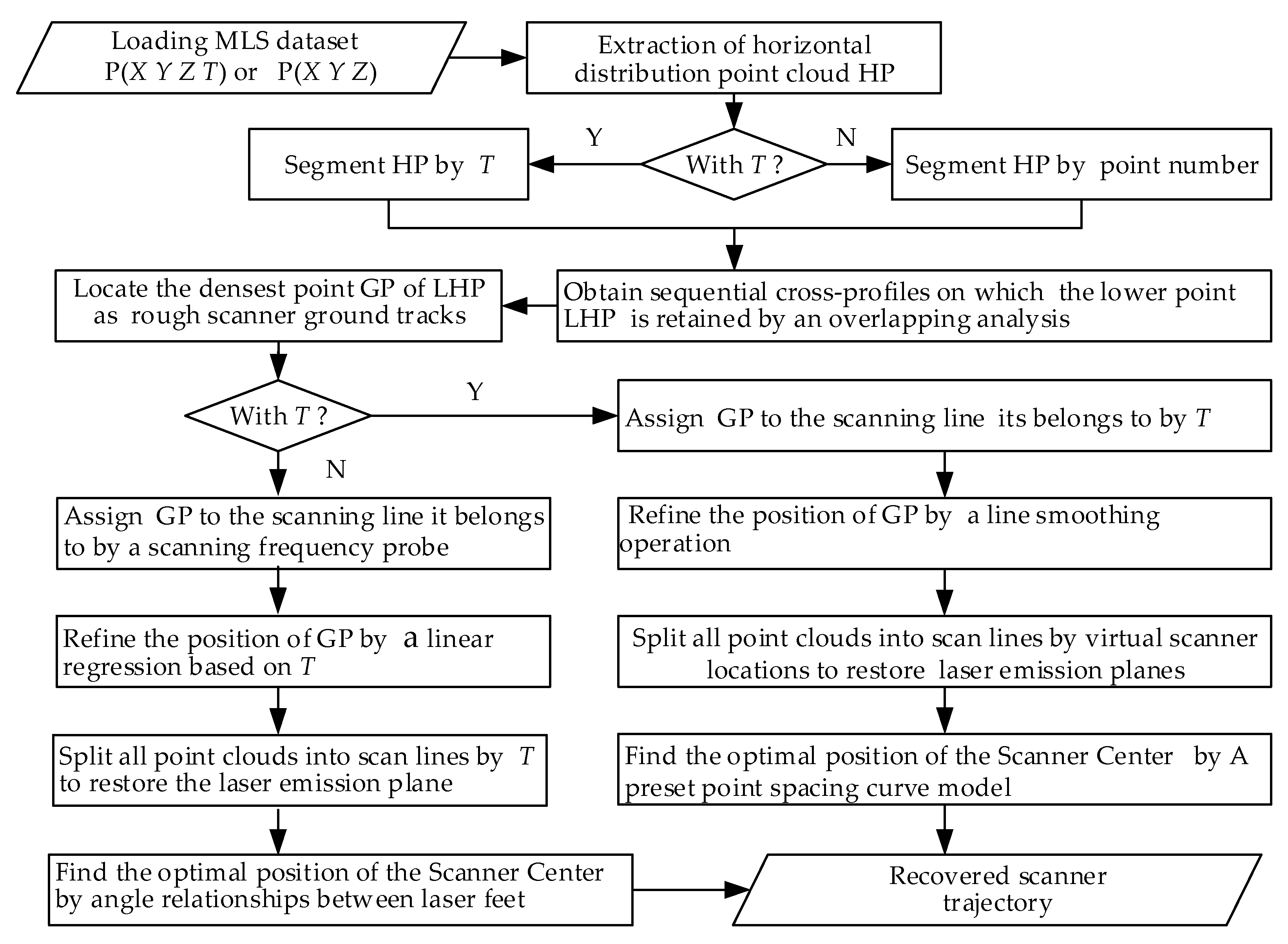
2. Methodology

Point density is an important attribute reflecting the degree of aggregation of a laser foot point. For data collected by a rotating mirror line scanning system, the point density decreases with distance from the scanner [45]. Because the road is close to the MLS, its surface points account for a large part of MLS data [46,47]. In the rotating mirror scanning mode commonly assembled in MLS systems [48], the spacing between the laser points in the horizontal plane increases with the measurement distance. Assuming that the closest projection point of the scanner to the ground (hereinafter referred to as the scanner ground track) is located on a flat road, it is located at the position with the highest density on the road.

Figure 1 shows a flowchart of the process of recovering vehicle trajectory for two kinds of known conditions. The first input condition is (X,Y,Z,T), that is, in addition to the coordinate value (X,Y,Z) of the point data, the acquisition time T of the laser pulse returning to the MLS system is required. The second kind of condition includes only the coordinate values (X,Y,Z) of the point cloud recorded by the acquisition sequence. In Figure 1, point set P represents the MLS point cloud dataset collected over time. This study first extracts rough road points HP using a horizontal distribution detector, and then conducts upper and lower overlapping analyses of the local point section to remove possible point clouds over the road surface. The remaining point clouds are recorded with the data set LHP. A rough ground track of the scanner GP is determined by point density and refined by different models according to two kinds of known conditions. The point cloud is then divided into scanning lines to recover the laser scanning plane, in which the center of emission of the scanner is reconstructed by the angles or spacing between laser points.

2.1. Based on Three-Dimensional (3D) Coordinates and Acquisition Time of Point Cloud

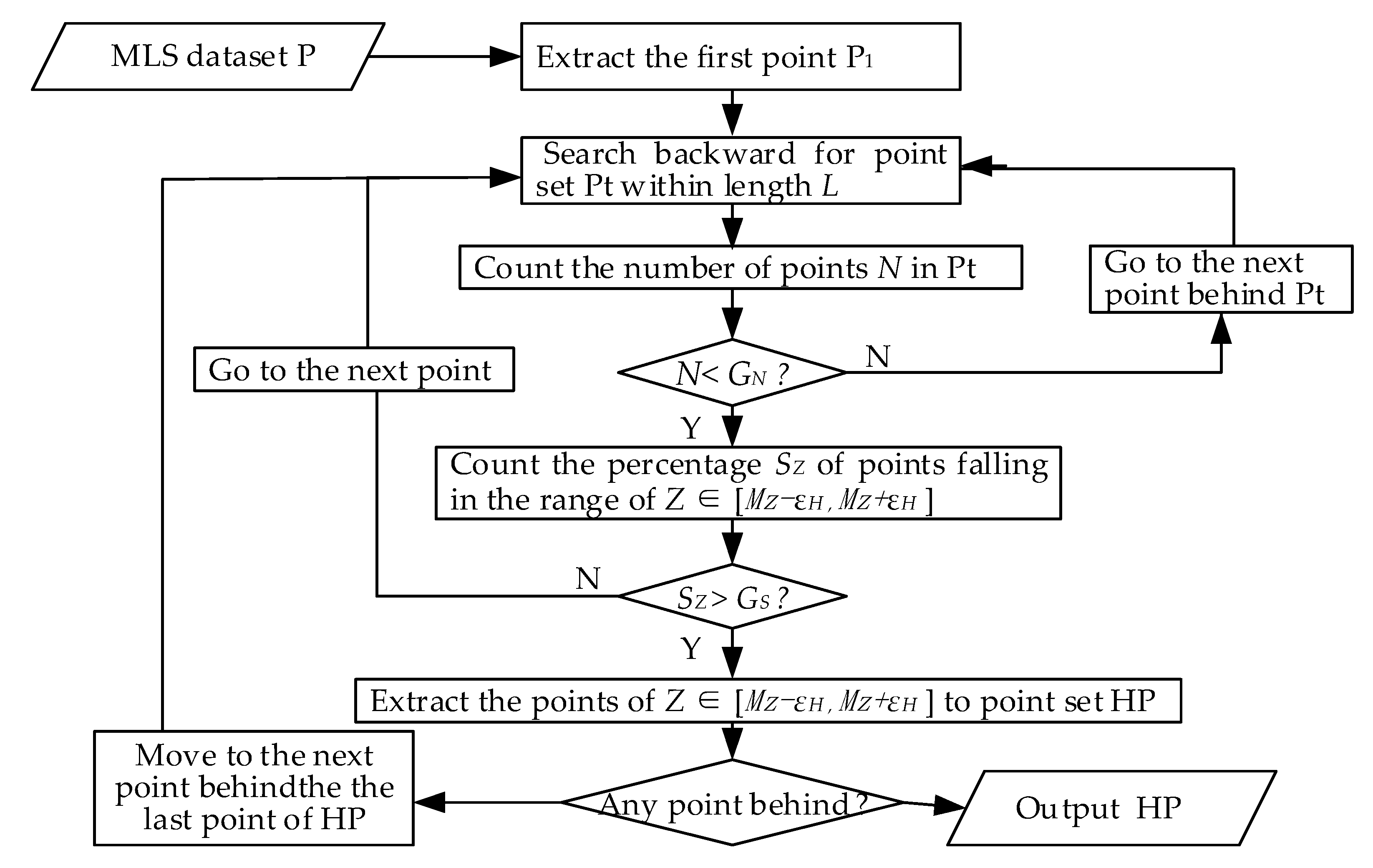
2.1.1. Rough Road Point Extraction

Suppose the point cloud collected over time by the MLS system is stored in dataset P in the recording format(X,Y,Z,T). Figure 2 describes the detailed process of rough road point extraction.

The process is carried out according to the order of data collection. A horizontal distribution detector is designed and placed at the first point (P₁) of P. The point backward is searched along the recording sequence to find the first one to reach L (Euclidean distance) to P₁. Let it be the Nth one. The dataset Pt = {P₁, P₂, …, P_N} forms a temporary data segment. We set a threshold G_N for the number of points in Pt. If N < G_N, we discard this segment Pt; otherwise, we set a height difference threshold ε_H with the elevation median Mz of Pt point as center. The percentage S_Z of points within the range [Mz − ε_H, Mz + ε_H] in Pt is counted. If S_Z > G_S, Pt contains points conforming to the horizontal distribution, where G_S is a preset percentage. Then, the points of Z∈ [Mz − ε_H, Mz + ε_H] are extracted and placed in the horizontal distribution point set HP. The next judgment point is moved to the one following HP. On the contrary, if Pt does not conform to a horizontal distribution, only one position is moved backward as the next judgment point.

The length of search L was set to 2 m in this study, according to the width of the average vehicle, because the point cloud directly below the vehicle must be part of the road. The height difference threshold ε_H was set at 0.1 m according to the maximum cross-slope in Chinese road design specifications. Owing to the point density of MLS data, there are generally dozens to hundreds of road points within L (2 m in this study). We set G_N = 10, G_S = 0.9, i.e., 10% noise points were allowed. The proposed algorithm has the advantages of simplicity, feasibility, low computation cost, and wide applicability. In addition, the point cloud of the road accounted for a large part of MLS data. The road segment uses L as a judgment step, thus speeding-up processing.

2.1.2. Road Point Filtering

HP may contain an upper point over the road from the viaduct, traffic sign, height limit pole, or the power line, which might have a higher point density as such points are closer to the laser scanner. To remove them, we convert HP to cross profiles, within which the point clouds over the road can be distinguished. As the direction of cross profiles are constantly changing, HP is divided into different segments according to the acquisition time T. Let t_s be the time difference of point cloud included in each segment and the i^th segment is marked as SHP_i. SHP_i = {HP ((i − 1) t_s < T_i − T₁ ≤ i t_s)}, i = 1, 2, …, k, where k is the total number of segments. $k=\lceil \raisebox{1ex}{$(T_{end}-T_1)$}\!\left/ \!\raisebox{-1ex}{$t_s$}\right.\rceil$. T₁ and T_end represent the acquisition time of the first and the last point in HP, respectively. The point cloud in SHP_i keeps the original data structure (X,Y,Z,T). As the line acquisition frequency of MLS system is generally adjustable from 50 to 300 Hz, we set t_s = 0.05–0.1 s. Project SHP_i vertically onto a horizontal plane, that is, [X Y 0] = [X Y Z] [1 1 0]^T. Principal component analysis (PCA) is applied to obtain the unit eigenvector α₁ corresponding to the first principal component of the projection segment. Let α₁ = [l₁ l₂ 0]^T, α₁ represent the general direction of a scan line. We focus on the orientation of the scanning line, and not the direction of the vector. The two vector orientations with an included angle of π are identical. The orientation vector α₁' of α₁ can be expressed as: α₁' = [sgn(l₁)l₁ sgn(l₁)l₂ 0]^T. A coordinate transformation is implemented on SHP_i with α₁ as X’-axis and the Z-axis unchanged. The transformation matrix M can be expressed by Equation (1):

$$M=\left[\begin{array}{ccc}\mathrm{sgn}(l_1)l_1& \mathrm{sgn}(l_1)l_2& 0\\ -\mathrm{sgn}(l_1)l_2& \mathrm{sgn}(l_1)l_1& 0\\ 0& 0& 1\end{array}\right]$$

(1)

After conversion, the coordinates of point in SHP_i are (X’,Y’,Z). Figure 3 shows the point distribution of SHP_i in the X’ Y’ and X’ Z planes. The red point represents the candidate road point, and the blue points are the segment points of the original data P after segmentation and transformation using the same time interval t_s to illustrate the positions of the red points.

Figure 3b shows the vertical profile along the scan line. The range of red points on the X’-axis is calculated and a movable vertical window XM = [X_a’, X_b’] is applied from the far left, where X_b’ − X_a’ stands for interval width. The point in XM is vertically stratified several layers from the lowest point within. If there are overlapping layers in the upper part of XM, they are filtered out, and only the lowest layer is retained. The interval width X_b’ − X_a’ and height of the layer can be set according to the size of an ordinary car. In this study, we used 2 m and 1.2 m, respectively. The moving window slides from left to right across the candidate road points (red points in Figure 3b) with a step size of 1 m. The reserved lower-layer point is recorded in the point set LHP_i, i.e., the ith segment point cloud after filtering.

2.1.3. Point Density Analysis to Roughly Locate Scanner Ground Tracks

Assuming that the closest laser foot point to the laser scanner is on the road, it can be located using the point density feature within LHP_i. We search for the number of neighboring points (N_R) in the R range of each point along the order of recording. The value of N_R reflects the point density along the scan line, which is relatively stable and is not affected by the variation in scan line spacing due to the change in driving speed. Figure 4 shows the distribution of laser foot points on the horizontal ground in a single scanning line. The smallest distance between the laser scanner and the ground is expressed in H. Let θ and ∆θ express the instantaneous scanning angle of the emitted laser beam and resolution of the scanning angle of the rotating mirror system, respectively. The spacing between adjacent laser foot points in a scanning line on the completely horizontal ground ∆s can be expressed as Equation (2):

$$\mathsf{\Delta }s=\frac{H\mathsf{\Delta }\mathsf{\theta }}{\cos \mathsf{\theta }}$$

(2)

Given the range of neighborhood search R = 1 m, the point density N_R is inversely proportional to point spacing ∆s. Equation (2) can then be expressed as: N_R = (H∆θ)⁻¹cosθ. The point density N_R yields its maximum value N_R max when θ = 0. However, the road surface is not completely horizontal. As shown in Figure 4, if there is a small fluctuation h in the local area, the spacing ∆s changes, because of which the peak value N_Rmax may not obtain at the point nearest to the scanner. In this study, a high-density area is extracted from the adaptive threshold th_N, and the location of the scanner’s ground track is represented by coordinates of the regional barycenter. Threshold th_N can be determined according to the normal installation height H of the laser scanner and lane width B. The width of a typical Chinese road lane B is generally 3.5–3.75 m. We set H to be 3 m according to the general installation height of the MLS systems. Assuming that the vehicle was moving in the middle of the lane, the scanning angle of the lane boundary can be calculated as θ = arctan(B/(2H)). The value of the scanning angle θ is approximately 35 degrees according to the specified values of H and B. Point density N_R due to the scanning angle θ decreases to cosθ times N_Rmax. From the above, the point density threshold th_N was set to th_N = 0.8 N_Rmax, where the constant coefficient 0.8 was derived from the cosine of the scanning angle at the lane boundary. The point below the vehicle belongs to the road. All points satisfying N_R > th_N in LHP_i are extracted to form the road feature area PN_i, and the barycenter coordinate G_i is calculated as $G_i(X_0,Y_0,Z_0)=\overline{P{N}_i(X,Y,Z)}$. The nearest point GP_i in LHP_i to G_i is determined by Euclidean distance $d_i=\sqrt{{(X_i-X_0)}^2+{(Y_i-Y_0)}^2}$. Point set GP forms the scanner’s rough ground trajectory.

2.1.4. Refinement of Scanner’s Ground Trajectory

For a 2D line laser sensor, the elapsed time on each scanning line is equal, as long as the scanning speed (scanning line frequency) is set. All scanner ground tracks measured the laser foot points corresponding to the same scanning angle. Their time interval is a multiple of the elapsed time on each scan line. Let t_d be the elapsed time on each scanning line. The acquisition time of the scanner ground tracks (T_Gi) satisfy an isochromatic sequence of Equation (3).

$$T_G{}_i=t_1+(SN{l}_i-1)\times t_d$$

(3)

where T_Gi represents the acquisition time of the GP_i, i.e., the ith point of the scanner’s ground tracks. SNl_i records the scanning line number to which GP_i belongs, where the first point in P belongs to the first scanning line. Let t₁ denote the acquisition time of the scanner’s ground track on first scanning line, and t_d is the elapsed time on each scanning line. To estimate t_d, we take any two adjacent points from GP—as shown in Figure 5—take the line between GP_i-1 and GP_i as center, expand the area of the scanning frequency probe by a width of several laser points (such as 0.2 m), and extract the point cloud in the probed area.

There is little difference in acquisition time T among points 1–4, 5–8, and 9–12 owing to their recording relationships. However, there is a mutation in time difference at 4–5 and 8–9, which is hundreds of times that at the front. The time difference of the mutation t_l is taken as the approximate t_d. In Figure 5, t_l ≈ T₅ − T₄. The number of scan lines subordinate to point GP_i can be determined by Equation (4):

$$SN{l}_i=1+\lfloor \frac{T_G{}_i-T_{G1}}{t_l}+\frac{1}{2}\rfloor$$

(4)

With SNl_i, we take T_Gi as the measurement with errors. A linear regression is carried out to obtain reliable estimation parameters t₁ and t_d from Equation (3). Then, the estimated values of t₁ and t_d are carried into Equation (5) to solve for the acquisition time t_i of the scanner’s ground tracks on each scanning line.

$$t_i=t_1+(n-1)\times t_d$$

(5)

where, n∈(1,SLN_end), and SLN_end represents the serial number of the scanning line of the last point of the original data P, calculated by Equation (6):

$$SL{N}_{\mathrm{end}}=\lfloor \frac{T_{\mathrm{end}}-T_{G1}}{t_d}+\frac{1}{2}\rfloor$$

(6)

Finally, the point the acquisition time T of which is closest to t_i is extracted as the recovered ground track of the scanner.

2.1.5. Reconstruction of Scanner Trajectory

For a 2D single laser scanner system, the laser foot point (the yellow point shown in Figure 6a) on a single scanning line (green dotted line) is located in a scanning plane as shown in Figure 6b. The scanning plane can thus be reconstructed by the point cloud on each scanning line. In [20], the point cloud was split into scanning lines using the jump in time difference between adjacent laser points. Considering that there may be objects over the scanning vehicle, this study uses the reliable estimation of the t_i and d_t of the ground track points obtained in Section 2.1.4 to roughly divide the points in P into each scanning line by [t_i − d_t/2, t_i + d_t/2].

Suppose there are N_L points on a scan line. The coordinate vector v_i = (X_i Y_i Z_i), i = 1, 2, …, N_L makes up the covariance matrix A. Let the center of the point set on this scanning line be m, $m={\displaystyle \sum _1^{NL}(X_i,Y_i,Z_i)}/N_L$. Then, the eigenvector corresponding to the minimum eigenvalue λmin of A represents the normal vector N of the scanning plane [49]. Considering the point cloud underneath the vehicle, we take the point within 0.5 m from the scanner’s ground track point on its scanning line as the local road section. PCA is used to obtain the maximum principal orientation S_L (using the process described in Section 2.1.2) of the local road section. S_L is taken as the x-axis, the normal vector N as the z-axis, and the direction of the cross-product S_V as the y-axis, S_V = S_L ⨂ N, to transform all scanning line points to the scanning plane. The transformation matrix M2 can be expressed as: M2 = [S_L^T; S_V^T; N^T].

Figure 7a shows the scanning plane (xz plane) reconstructed by a single scanning line. The center of emission of the scanner O should be located approximately over its ground track point. Let Snt_i(x₀, y₀, z₀)denote the scanner’s ground track transformed by M2, and O be preset to z_s higher than point Snt_i. The included angle ∠1O2 formed by connecting any two laser foot points 1 and 2 can be calculated by Equation (7). If multiple echoes points are not considered, the true value of ∠1O2 can be determined according to the ratio of the time difference recorded at 1 and 2, and $\angle 1\stackrel{⌢}{O}2=\frac{S{t}_2-S{t}_1}{t_d}\times 2\pi$, where St₁ and St₂ represent the acquisition times of any two laser foot points 1 and 2, respectively.

$$\angle 1O2=acos(\frac{a·b}{\left|a\right|\left|b\right|})$$

(7)

where $a=(x_1-x_0,z_1-z_0-z_s)$, $b=(x_2-x_0,y_2-y_0,z_2-z_0-z_s)$.

The analytical solution of O is complex. This research set an initial value for z_s according to the normal installation height of the scanner, near which a rectangular subdivision grid area (pink-filled area in Figure 7b of width 2bx and height z_max − z_min) was established. The resolution of the subdivision grid was set to 0.01–0.05 m, as a higher resolution was unnecessary due to system error, the normal vector error of the estimated plane, and other errors. We set bx to be 0.3 m as Snt_i deviates little from the scanner’s ground track. z_min and z_max were determined as 3 m, 2 m, and 6 m, respectively, based on the general height of the vehicle.

To reduce the number of observation equations, the scanning plane can be divided into areas in several directions (such as the 18 directional areas shown in Figure 6a). If there are laser foot points in a directional area, the farthest point from O(x₀, z_s + z₀)is recommended to represent the area to improve the accuracy of direction. We take the zenith (vertical upward) as the 0 direction, and the other directions are calculated in order of acquisition time. The angle between the last direction and the first (time difference is negative) does not participate in the subsequent procedure. The observation angle is formed at any two directions. The optimal solution of O is determined by ${\displaystyle \sum _1^{N_K}}\left|\angle 1\stackrel{⌢}{\mathrm{O}}{2}_i-\angle 1\mathrm{O}{2}_i\right|=\min$, where N_K is the number of angles included in the calculation. The scanner’s position is finally recovered by using the inverse matrix of M2 and optimal grid coordinates of O.

However, the MLS data may contain points with multiple echoes. It is necessary to remove this part of the point cloud before recovering the scanner’s center of emission O. This study determines the multiple echo points using acquisition time T. Figure 8 describes a schematic diagram of the laser’s transmitting and receiving times. The block represents the time of laser emission, the dot the time of echo reception, ∆t denotes the laser’s emission interval constant during data acquisition, and t_R1, t_R2, and t_R3 represent the intervals of three consecutive main waves received. In Figure 8, two echoes are detected in the first and third laser emission intervals, and no echo is detected in the fourth laser emission interval.

Points with multiple echoes or no echo took up a small portion of the road point data. The interval between adjacent points was mostly consistent with ∆t. The process of detecting multiple echoes is as follows:

• Calculate the time interval between adjacent points in the LHP to obtain sequence ∆T.
• Statistically analyze ∆T and take the first quartile Q1 as an approximation of the laser’s emission interval ∆t because the percentage of the laser beam without echo in road point cloud is generally less than 25%.
• Mark the number of emissions of the first point of P as 1, and calculate the number of emissions of the other point using Equation (8):

  $$S{N}_i=\lfloor \frac{T_i-T_1}{\mathsf{\Delta }t}+\frac{1}{2}\rfloor$$

  (8)

  where SN_i represents the number of emissions of the ith point in P.
• Calculate the difference in SN_i. The points satisfying SN_i − SN_i-1 = 0 are multiple echo points. Remove them to facilitate subsequent data processing.

2.2. Based on Ordered 3D Coordinates of Point Cloud

A point set with only coordinates (X,Y,Z), P can be segmented according to the number of points. Current MLS systems emit thousands of points per scanning line. We take out tens of thousands of points to ensure that multiple scanning lines are crossed. Then, the scanner’s ground trajectory GP_i is extracted by a method similar to that described in Section 2.1.2. The next step is to refine these data and divide the points of P into scan lines. For convenience of explanation, we add a column NO to P, P = {X Y Z NO}, where NO represents the serial numbers of points in P.

2.2.1. Refinement of Scanner’s Ground Trajectory

The vehicle’s travel path should be smooth. The scanner’s ground trajectory based on the center of gravity of density can be refined by a smooth line operation. Figure 8 illustrates the process of refinement. The red dot represents the scanner’s rough ground track point GP_i. To refine its position. A neighborhood point within a certain distance, such as 0.5 m from GP_i, is extracted to regress a straight line (black line in Figure 9) using the least squares method. An adjustment domain is built before and after GP_i, for example, 30 points (in the green box in Figure 9), and the point closest to the regression line (black) is used to refine the position of GP_i. The refinement of GP_i is still subordinate to the original data P.

2.2.2. Separating Point Clouds into Scanning Lines

To separate the point data of P into different scanning lines, we use the virtual scanner location method. A segment divided by the number of points is extracted and transformed into an approximate cross-profile using the procedure in Section 2.1.2. A virtual scanner center VO is created 3 m (set by the general mounting height of the MLS systems) over GP_i inside the X’Z plane to calculate the zenith angle w of each point (X’,Y’,Z) using Equation (9). Let (X_V’,Y_V’,Z_V) be the coordinates of VO in the approximate cross-profile:

$$\mathsf{\omega }=\arctan (\frac{Z-Z_{\mathrm{V}}{}^{\prime }}{(X^{\prime }-X_{\mathrm{V}}{}^{\prime })})+C$$

(9)

where C is a constant to extend the range of w to (0,2π), and its value is calculated as follows:

$$C=\{\begin{array}{ccc}0& & X^{\prime }\ge X_{\mathrm{V}} \& Z\ge Z_{\mathrm{V}}\\ \pi & & X^{\prime }<X_{\mathrm{V}}\\ 2\pi & & X^{\prime }>X_{\mathrm{V}} \& Z<Z_{\mathrm{V}}\end{array}$$

(10)

We then detect the points of w crossing from one side of zero to the other, and record their serial numbers NO into a branching number sequence BL. The point cloud between the transitions is assigned to a scanning line. Note that this division is approximate. Some points belong to two scan lines or no scan line. However, the result is not affected as only the road point is used in the next step.

2.2.3. Reconstruction of Scanner Trajectory

After separating the point data into scanning lines, the scan plane can be reconstructed using a process similar to that in Section 2.1.5. In this section, the location of the scanner’s center of emission O is reconstructed according to the spacing between adjacent points on the road. Assuming that the road surface is horizontal, Equation (2) is deformed to a radical function about ∆s and ∆x, where ∆x is the spacing between a laser foot point and the ground track point Snt_i(x₀, y₀, z₀)along the X-axis. The function of ∆s on ∆x can be expressed as in formula (10):

$$\mathsf{\Delta }s=a\sqrt{{(\mathsf{\Delta }x-b)}^2+c^2}$$

(11)

where a represents a scale coefficient, a = cos∆θ; b is a correction coefficient of Snt_i in the x direction, and c describes the scanner’s height in the scan plane.

The points in LHP_i are also separated into scan lines according to the branching number sequence BL. The road points do not contain multiple echo data, but some points may be missing. To obtain a relatively reliable point spacing sequence ∆s, the median filtering method is applied. Its size can be specified by the number of points, such as five points or more. According to the results of the analysis Section 2.1.3, the point spacing ∆s in high-density areas is alike. We set different weights p for each road point according to ∆x, expressed as follows:

$$p=\{\begin{array}{ccc}1& \left|\mathsf{\Delta }x\right|\le 1& \\ \left|\mathsf{\Delta }x\right|& \left|\mathsf{\Delta }x\right|>1 \&& \left|\mathsf{\Delta }x\right|\le 6\\ 0& \left|\mathsf{\Delta }x\right|>6& \end{array}$$

(12)

The weighted least-squares method is used to solve for the extreme values of the point spacing curve, and to determine the optimal solutions of a, b, and c according to the observation equation listed using multiple observation values of ∆s and ∆x, as shown in Figure 10.

The resulting accuracy may not be as high as that in the first kind of input condition, due to the influence of the resolution of point coordinates and roughness of the road. However, the values of c are similar after the scanner is installed in place. To reduce noise, the value of c can be analyzed using a histogram. Values of c that deviate from the peak of the histogram by more than three times the mean square error were removed according to the measurement error theory, and the value of c of the adjacent scan line is used in its place. On roads with little change in the longitudinal gradient, the same c (peak value in the histogram) can be used to reconstruct all centers of the scanner.

3. Experiments

3.1. Test Data

To verify the validity and correctness of the proposed approaches, we selected point data for four typical road environments—urban, rural, winding, and viaduct—collected by two kinds of MLS equipment from different manufacturers. Two MLS systems integrate 2D scanners with rotating mirror line sweeps. The characteristics of each scene shown in

Table 1. Test data environment.

Test Data	Site	Line Type	Road Surface Evenness	Road Slope (%)	Road Width (m)
Data 1	urban	straight	even 1	H 3: 2, V 4: 3	8
Data 2	rural	curve	rough 2	H: 3, V: 5	3.0–4.5
Data 3	winding	curve	rough	H: 8, V: 10	6.0
Data 4	viaduct	curve	even	H: 2, V: 2	10.0

¹ Road surface is smooth and tidy, ² uneven and coarse road surface, ³ horizontal, ⁴ vertical.

and

Table 2. Test data features.

Test Data	Volume (Million Points)	Size (MB)	Road Length (m)	AS 1 (cm)	LS 2 (m)	PR 3 (%)	PM 4 (%)
Data 1	2.8	172	115	0.7	0.08	73	0.01
Data 2	3.6	235	120	0.9	0.11	60	0.05
Data 3	3.2	324	140	0.5	0.15	70	0.10
Data 4	2.1	217	130	0.4	0.08	87	5.14

¹ Average point spacing right below vehicle, ² scan line average spacing, ³ proportion of road point, ⁴ proportion of multi echo point.

describe the basic features of the four sets of data.

The first three pieces of data were collected by SSW Vehicle-Borne Mobile Modeling and Surveying System produced by Beijing Si-Wei Farsighted Information Technology Co., Ltd. Within seconds, 200,000–500,000 measurements and 50–250 scan lines are collected in a typical measurement range of 1–500 m with an angular accuracy of 0.1 milli-radians. A scanner with a 360-degree horizontal field of view is installed with a 45-degree inclination from the vertical direction. The scanner head faced directly behind the vehicle and the scanning line was perpendicular to the vehicle’s direction of motion. The last piece of data was collected by the “MyFlash” mobile measurement system (MMS) developed by Wuhan University and Leador Information Technology Co., Ltd. It is mounted in an oblique position at an angle of 65 degrees from the driving direction, causing the scanning line to deviate by 65 degrees from the vehicle’s direction of motion. Figure 11 shows test data for four typical environments rendered with point elevation.

3.2. Results

3.2.1. Road High Density Area and Scanner Ground Traces

The rough scanner ground tracks come from the density distribution of road point cloud. It is actually a kind of point density statistics based on the same scan line, which is not affected by the driving speed. In Figure 12, a progressive transition from blue to green, then to yellow, and finally to red is used to represent the distribution of road point density from low to high.

Two questions are pertinent: (1) Were other low-density points mixed in with the high-density area (in red)? (2) Were the high-density points clearly distinguishable from the low-density area? Question (1) can be answered by examining the purity of the red points. As shown in Figure 12, Data 1 and Data 4 obtained a purer red area followed by Data 2 and Data 3. This result corresponds to the roughness of the road surface, which is an important factor affecting point density. Question (2) can be answered by examining the distinguishability of red and the other colors. Although the high-density areas of the four scenarios were distinguishable from the surrounding point clouds, the red area in Data 2 reached the boundary of the road in some parts, whereas a distance was maintained between the point clouds and the edge of the roads in the other scenarios. Both the above aspects can cause the scanner’s rough ground trajectory (blue point in Figure 13) of the high-density area to swing in the road. The first situation leads to the incomplete extraction of the high-density area, and the second one leads to missing data in areas of the road outside the high-density area.

The blue point in Figure 13 represents the scanner’s rough ground track of the high-density area in each scanning line. Figure 13a,b show good results even when the steps of refinement were not implemented. The scanner’s rough ground track in Data 3 oscillated as the vehicle moved. However, all values were close to the real trajectory (black line) with little deviation. The maximum deviation occurred in one segment in Data 2 as shown in Figure 13d. Although the blue points were close to one another, they deviated from the empirical trajectory as a whole owing to a sudden narrowing of the road.

As shown in Figure 14, the effects of the deviations in Data 2 and Data 3 were corrected by using the first kind of known condition (green points in Figure 14a,b). The second kind of known condition was used to quell the stumbling and fluctuating of the distribution of local points (magenta points in Figure 13a). The overall offsets (Figure 14b) could not be corrected with the second kind of input conditions.

We compared two results with the true value extracted from the position of the laser foot point corresponding to the scanning angle zero provided by the system’s data processing software. Two comparative results of the larger deviations of Data 3 and Data 2 are shown in Figure 15.

As shown in Figure 15, the first input condition obtained excellent accuracy. The deviation was very small and, on average, differed by only a few centimeters from the true value. The result was even better for Data 1 and Data 4 (controlled within 0.01 m). There was a sharp contrast in the range of deviation between the two kinds of input conditions. The first one produced a uniform, small, positive or negative deviation while the second result fluctuated considerably. In the second kind of input condition, the maximum deviation occurred on the rural road in Data 2. The maximum deviation along the scan line was 0.175 m, approximately 20 laser points. However, the variance of deviation was controlled at 0.0137 m—approximately two laser points—indicating that centimeter-level accuracy was guaranteed. The line smoothing method is thus effective for shocks near the true value but slightly far-fetched in some special cases, which are introduced below.

3.2.2. Reconstructed Scanner Track

In Figure 16, the red and blue colors represent the scanner’s tracks restored by the first and second input conditions, respectively. The cyan line between the ground track point and the center of laser scanning illustrates the scanning plane sampled for display effect. The original data are rendered with intensity information. To evaluate the accuracy of the data, the point closest to the time tag in the sequence of the scanner’s centers of emission calculated by GPS and integrated inertial navigation data was selected as the true value.

Table 3. Comparison between the recovered center of emission of laser and the true value.

Test Data	Statistical Deviation	XY 1 (m)	Z 2 (m)	E 3 (m)	XY 4 (m)	Z 5 (m)	E 6 (m)
Data 1	Maximum Average Variance	0.034	0.093	0.094	0.103	0.141	0.151
		−0.003	0.031	0.031	−0.008	−0.089	0.089
		0.004	0.009	0.010	0.012	0.013	0.016
Data 2	Maximum Average Variance	0.103	0.112	0.117	0.171	0.214	0.230
		0.026	0.039	0.041	0.033	0.040	0.046
		0.008	0.013	0.014	0.021	0.024	0.045
Data 3	Maximum Average Variance	0.055	0.107	0.102	0.157	0.149	0.171
		0.006	−0.012	0.013	0.024	0.027	0.032
		0.008	0.011	0.012	0.016	0.015	0.018
Data 4	Maximum Average Variance	0.016	0.011	0.017	0.062	0.070	0.073
		−0.007	0.004	0.008	−0.014	0.015	0.018
		0.003	0.004	0.004	0.008	0.010	0.010

¹ Horizontal and ² elevation deviation of the first input condition, ⁴ horizontal and ⁵ elevation deviation of the second input condition. ^3,6 Euclidean distance deviation of the first and second condition, respectively.

shows the statistical deviations.

For four research data, there is a general trend that the scanner’s center of emission recovered by the first input condition was closer to the true value than the second one, both in terms of variance and maximum deviation. In addition, there are a few gross errors in Data 2 while having considerable oscillations in Data 3 based on the second input condition. Thus, the recovery accuracy of these two data are not as good as Data 1 and Data 4. It is possible that the preset point spacing model may not conform to the real ones, which may lead to systematic errors. However, both methods have achieved satisfactory results. Data 2 still recorded the largest deviation while Data 4 obtained the highest accuracy (variance within 1 cm). The maximum deviations for the two kinds of input conditions were 0.117 m and 0.230 m, respectively. The minimum variance was about 0.045 m, and most of the errors were controlled to within 0.1 m.

4. Analysis and Discussion

Two approaches were implemented in MATLAB running on an Intel (R) Core (TM) i7-7700 computer with 16.0-GB memory. Four pieces of data cover 200–300 m with 2000–3600 scanning lines. Based on the first and second conditions, it takes up to 2.1 and 2.5 minutes, respectively, to extract rough scanner tracks and up to 2.0 and 0.6 minutes, respectively, to restore scanner trajectory. As the extraction procedure is in accordance with the original record order of point cloud, the recovery method obtains a very fast processing efficiency.

The experimental results of the two kinds of input conditions verified the correctness and effectiveness of the proposed approaches. However, based on different principles, the reliability of the approaches varied. In the following, four factors are analyzed: Road line type, road conditions, position of scanner installation, and environment around the road.

4.1. Road Line Type

The four roads that we studied can be divided into three categories—straight line (Data 1), general curve (Data 2, Data 4), and bent (Data 3)—according to road line type. The rough ground trajectory was acquired by using the high-density area in the scanning lines independent of line type. The first kind of input condition refined it based on an isochromatic sequence of acquisition time insensitive to curves in the road while the second was based on line smoothing, and smoothened local oscillation through neighborhood track points of multiple scan lines. Figure 17 illustrates a polyline effect widely observed in the linear regression algorithm. The blue and red dots represent the results before and after refinement, respectively, and the green lines describes line segments to which the blue points conformed. This phenomenon was more prominent in bends with a large radius of curvature and not significant on straight-line road sections.

In general, the larger the neighborhood participating in line fitting is, the more prominent this phenomenon is. The neighborhood radius was set to 0.5 m in Figure 17 to achieve a relatively smooth curve. However, a large smooth radius can offset the oscillation slot of local traces to be more consistent with the overall route, while a smaller radius can only partially adjust the position of the track points. Therefore, the selection of neighborhood radius should be adaptive and is worth exploring. We will consider this in future research. The recovery of the scanner’s center of emission was based on a scan plane reconstructed by a single scan line, which was not directly associated with road line type.

4.2. Road Conditions

The road conditions discussed here include the slope, width, and evenness of the road. The effect of slopes was not reflected in the experimental results. Width is an important factor in two cases: (1) Determining the threshold of the high-density area, and (2) fitting the curve of the radial function based on the point spacing of the road. In Data 2, the minimum rural road shrunk to a width of 3 m, smaller than the preset lane width of 3.5 m. The boundary effect (edge of high-density areas coinciding with the boundary of the road) caused the density center of gravity to deviate from the original path, which could not be corrected by the line smoothing method. The second kind of input conditions recovered the scanner’s center of emission based on the curve fitting of the radial function of point spacing. A wider road caused the point spacing to have a wider range, resulting in more robust and reliable results of curve fitting. On the contrary, if the road was too narrow and the high-density area reached its boundary, the close point spacing was not conducive to the fitting algorithm. However, road width was not the only factor influencing high-density areas. The unevenness of the road surface rendered the aggregation of points ambiguous on narrow roads. The results show that the roughness of the four types of roads was positively related to the deviation of the estimated trajectory. The higher road roughness was, the larger the deviation was in the recovered trajectory. In Data 3, it is clear that roughness caused the center of gravity of the high-density area to swing. However, based on the linear regression of acquisition time, the first kind of known condition dispersed the deviation in each scan line to obtain the desired results. The second kind of known condition controlled local deviation and reduced the amplitude of swing to cause the recovered trajectory to converge to the true value.

4.3. Position of Scanner Installation

The two kinds of approaches to recovering the trajectory of the scanner considered here imposed no limitation on the position of the scanner. However, the inclination angle of the scanner may cause the nearest ground projection point to it to be outside the road. In this case, neither method works. In addition, it is better to leave a certain distance between the road boundary and the scanner’s ground tracks to ensure that the road is wide enough to analyze the density and spacing of points on it.

4.4. Environment Surrounding the Road

As shown in Figure 18, the environment was relatively open, and featured farmland in Data 2, but was crowded in rural residential areas, cities, and in mountainous areas. We used points in a scan line to reconstruct the plane of laser emission when all entire laser foot points were located under the vehicle as shown in Figure 18b. In this case, the accuracy of the plane’s normal vector might be insufficient. Similar cases obtained in the viaduct of Data 4, where the angle span formed by the laser foot point in the scanning plane was small. A smaller fraction of the directional region must be applied to obtain a sufficient number of included angle equations to recover the scanner’s center of emission.

Considering that sides of the road are invariably elevated, all data recorded did not feature open space as shown in Figure 18b. The heights of the scanner’s centers of emission were similar on roads, with little changes in the longitudinal gradient. Histogram analysis was applied to scanner elevations z_s and c, and the peak value was extracted and extended to all scan lines.

In summary, the first approach proposed here can obtain an accurate ground trajectory of the scanner, with only a small deviation and uniform precision. The outstanding feature of the first condition is that the scanner trace in subsequent data can be derived directly from the obtained time difference as long as the data belong to the same scanning. This advantage renders the first input condition to be superior to the second. By requiring only the 3D coordinates of the sequential point data, the second approach can also obtain reliable results. The majority of error in the recovered track of the scanner was controlled to within 1 decimeter, which is sufficient for most applications.

5. Conclusions

Vehicle trajectories are useful for preprocessing MLS data. By focusing on certain cases where the trajectory data are unavailable, this study proposed recovering the scanner’s trajectory from MLS point data based on two general input conditions. First, rough ground tracks of the scanner were located by the point density of the road and refined based on an isochromatic sequence of acquisition times or a line smoothing operation. Second, the raw data were split into different scanning lines to reconstruct the scanning planes, where different models were used to locate the laser scanner’s center of emission. The results of experiments on MLS systems from two manufacturers prove the effectiveness of the proposed method. The recovered ground trajectory of the scanner deviated is only by a few laser feet from the actual position, and most of its reconstructed traces of emission were accurate to within 1 decimeter. An analysis of the results showed that the proposed method is more suitable for cases where the scanner is in a vertical position to inclined assembly. The effect of road conditions on the accuracy of the recovered trajectory was found to be more significant than those of the road line type, and environment. This study was limited by the absence of an effective solution to the phenomenon of local offset of scanner ground tracks by the second input condition, when encountering a narrow road. Notwithstanding these limitations, this result has shown that the recovered scanner ground tracks can meet the common uses of trajectory data as effectively as the vehicle trajectory, such as segmenting MLS data, providing the direction of local coordinate systems, helping separate the target from the point cloud of the background, and so on. For future studies, it would be interesting to expand other applications of trajectory data that are more useful for MLS data processing, such as, to establish time-based neighborhood relationship of point cloud based on the acquisition time of the scanner ground tracks and different scanning lines. We hope the new neighborhood relationship will be helpful to the rapid description of the local feature of point cloud and the deep learning of MLS data.

References

- Xiang, B.; Tu, J.; Yao, J.; Li, L. A Novel Octree-Based 3-D Fully Convolutional Neural Network for Point Cloud Classification in Road Environment. IEEE Trans. Geosci. Remote Sens. 2019, 57, 7799–7818. [Google Scholar] [CrossRef]
- El-Halawany, S.I.; Lichti, D.D. Detecting road poles from mobile terrestrial laser scanning data. GIScience Remote Sens. 2013, 50, 704–722. [Google Scholar] [CrossRef]
- Wen, C.L.; You, C.B.; Wu, H.; Wang, C.; Fan, X.L.; Li, J. Recovery of urban 3D road boundary via multi-source data. ISPRS J. Photogramm. Remote Sens. 2019, 156, 184–201. [Google Scholar] [CrossRef]
- Zhang, Z.; Sun, L.; Zhong, R.; Chen, D.; Xu, Z.; Wang, C.; Qin, C.; Sun, H.; Li, R. 3-D Deep Feature Construction for Mobile Laser Scanning Point Cloud Registration. IEEE Geosci. Remote Sens. Lett. 2019, 16, 1904–1908. [Google Scholar] [CrossRef]
- Gargoum, S.A.; El Basyouny, K. A literature synthesis of LiDAR applications in transportation: Feature extraction and geometric assessments of highways. GIScience Remote Sens. 2019, 56, 864–893. [Google Scholar] [CrossRef]
- Yang, B.; Liu, Y.; Dong, Z.; Liang, F.; Li, B.; Peng, X. 3D local feature BKD to extract road information from mobile laser scanning point clouds. ISPRS J. Photogramm. Remote Sens. 2017, 130, 329–343. [Google Scholar] [CrossRef]
- Yang, B.; Dong, Z.; Liu, Y.; Liang, F.; Wang, Y. Computing multiple aggregation levels and contextual features for road facilities recognition using mobile laser scanning data. ISPRS J. Photogramm. Remote Sens. 2017, 126, 180–194. [Google Scholar] [CrossRef]
- Wu, B.; Yu, B.; Huang, C.; Wu, Q.; Wu, J. Automated extraction of ground surface along urban roads from mobile laser scanning point clouds. Remote Sens. Lett. 2016, 7, 170–179. [Google Scholar] [CrossRef]
- Holopainen, M.; Kankare, V.; Vastaranta, M.; Liang, X.; Lin, Y.; Vaaja, M.; Yu, X.; Hyyppä, J.; Hyyppä, H.; Kaartinen, H.; et al. Tree mapping using airborne, terrestrial and mobile laser scanning—A case study in a heterogeneous urban forest. Urban For. Urban Green. 2013, 12, 546–553. [Google Scholar] [CrossRef]
- Yang, B.; Wei, Z.; Li, Q.; Li, J. Automated extraction of street-scene objects from mobile lidar point clouds. Int. J. Remote Sens. 2012, 33, 5839–5861. [Google Scholar] [CrossRef]
- Ma, L.; Li, Y.; Li, J.; Wang, C.; Wang, R.; Chapman, M. Mobile Laser Scanned Point-Clouds for Road Object Detection and Extraction: A Review. Remote Sens. 2018, 10, 1531. [Google Scholar] [CrossRef] [Green Version]
- Yadav, M.; Singh, A.K.; Lohani, B. Extraction of road surface from mobile LiDAR data of complex road environment. Int. J. Remote Sens. 2017, 38, 4655–4682. [Google Scholar] [CrossRef]
- Hanyun, W.; Huan, L.; Chenglu, W.; Jun, C.; Peng, L.; Yiping, C.; Cheng, W.; Li, J. Road Boundaries Detection Based on Local Normal Saliency From Mobile Laser Scanning Data. IEEE Geosci. Remote Sens. Lett. 2015, 12, 2085–2089. [Google Scholar] [CrossRef]
- Pu, S.; Rutzinger, M.; Vosselman, G.; Oude Elberink, S. Recognizing basic structures from mobile laser scanning data for road inventory studies. ISPRS J. Photogramm. Remote Sens. 2011, 66, S28–S39. [Google Scholar] [CrossRef]
- Zai, D.; Guo, Y.; Li, J.; Luo, H.; Cheng, W. 3D Road Surface Extraction From Mobile Laser Scanning Point Clouds. In Proceedings of the IEEE International Geoscience and Remote Sensing Symposium (IGARSS), Beijing, China, 10–15 July 2016; pp. 1595–1598. [Google Scholar]
- Zai, D.; Li, J.; Guo, Y.; Cheng, M.; Lin, Y.; Luo, H.; Wang, C. 3-D Road Boundary Extraction From Mobile Laser Scanning Data via Supervoxels and Graph Cuts. IEEE Trans. Intell. Transp. Syst. 2018, 19, 802–813. [Google Scholar] [CrossRef]
- Teo, T.-A.; Chiu, C.-M. Pole-Like Road Object Detection from Mobile Lidar System Using a Coarse-to-Fine Approach. IEEE J. Sel. Top. Appl. Earth Obs. Remote Sens. 2015, 8, 4805–4818. [Google Scholar] [CrossRef]
- Balado, J.; Martinez-Sanchez, J.; Arias, P.; Novo, A. Road Environment Semantic Segmentation with Deep Learning from MLS Point Cloud Data. Sensors 2019, 19. [Google Scholar] [CrossRef] [Green Version]
- Balado, J.; Díaz-Vilariño, L.; Arias, P.; Garrido, I. Point clouds to indoor/outdoor accessibility diagnosis. ISPRS Ann. Photogramm. Remote Sens. Spat. Inf. Sci. 2017, IV-2/W4, 287–293. [Google Scholar] [CrossRef] [Green Version]
- Yang, B.; Fang, L.; Li, J. Semi-automated extraction and delineation of 3D roads of street scene from mobile laser scanning point clouds. ISPRS J. Photogramm. Remote Sens. 2013, 79, 80–93. [Google Scholar] [CrossRef]
- Jung, J.; Che, E.; Olsen, M.J.; Parrish, C. Efficient and robust lane marking extraction from mobile lidar point clouds. ISPRS J. Photogramm. Remote Sens. 2019, 147, 1–18. [Google Scholar] [CrossRef]
- Rodríguez Cuenca, B.; García Cortés, S.; Ordóñez Galán, C.; Alonso, M.C.J. An approach to detect and delineate street curbs from MLS 3D point cloud data. Autom. Constr. 2015, 51, 103–112. [Google Scholar] [CrossRef]
- Wu, B.; Yu, B.; Yue, W.; Shu, S.; Tan, W.; Hu, C.; Huang, Y.; Wu, J.; Liu, H. A Voxel-Based Method for Automated Identification and Morphological Parameters Estimation of Individual Street Trees from Mobile Laser Scanning Data. Remote Sens. 2013, 5, 584–611. [Google Scholar] [CrossRef] [Green Version]
- McElhinney, C.P.; Kumar, P.; Cahalane, C.; McCarthy, T. Initial results from European road safety inspection (eursi) mobile mapping project. In International Archives of the Photogrammetry, Remote Sensing and Spatial Information Sciences; Vol. XXXVIII, Part 5 Commission V Symposium; International Society of Photogrammetry and Remote Sensing (ISPRS): Newcastle upon Tyne, UK, 2010; Available online: http://mural.maynoothuniversity.ie/9271/ (accessed on 10 March 2020).
- Holgado-Barco, A.; Gonzalez-Aguilera, D.; Arias-Sanchez, P.; Martinez-Sanchez, J. An automated approach to vertical road characterisation using mobile LiDAR systems: Longitudinal profiles and cross-sections. ISPRS J. Photogramm. Remote Sens. 2014, 96, 28–37. [Google Scholar] [CrossRef]
- Guan, H.; Li, J.; Yu, Y.; Wang, C.; Chapman, M.; Yang, B. Using mobile laser scanning data for automated extraction of road markings. ISPRS J. Photogramm. Remote Sens. 2014, 87, 93–107. [Google Scholar] [CrossRef]
- Guan, H.; Li, J.; Yu, Y.; Ji, Z.; Wang, C. Using Mobile LiDAR Data for Rapidly Updating Road Markings. IEEE Trans. Intell. Transp. Syst. 2015, 16, 2457–2466. [Google Scholar] [CrossRef]
- Guan, H.; Yu, Y.; Li, J.; Liu, P.; Zhao, H.; Wang, C. Automated extraction of manhole covers using mobile LiDAR data. Remote Sens. Lett. 2014, 5, 1042–1050. [Google Scholar] [CrossRef]
- Yu, Y.; Li, J.; Guan, H.; Jia, F.; Wang, C. Learning Hierarchical Features for Automated Extraction of Road Markings From 3-D Mobile LiDAR Point Clouds. IEEE J. Sel. Top. Appl. Earth Obs. Remote Sens. 2015, 8, 709–726. [Google Scholar] [CrossRef]
- Puente, I.; Akinci, B.; González-Jorge, H.; Díaz-Vilariño, L.; Arias, P. A semi-automated method for extracting vertical clearance and cross sections in tunnels using mobile LiDAR data. Tunn. Undergr. Space Technol. 2016, 59, 48–54. [Google Scholar] [CrossRef]
- Gargoum, S.; El-Basyouny, K. Automated Extractaion of Road Features Using LiDAR Data: A Review of LiDAR Applications in Transportation. In Proceedings of the 2017 4th International Conference on Transportation Information and Safety (ICTIS), Banff, AB, Canada, 8–10 August 2017; pp. 563–574. [Google Scholar] [CrossRef]
- Xin, C.; Kohlmeyer, B.; Stroila, M.; Alwar, N.; Bach, J. Next generation map making: Geo-referenced ground-level LIDAR point clouds for automatic retro-reflective road feature extraction. In Proceedings of the 17th ACM SIGSPATIAL International Symposium on Advances in Geographic Information Systems, ACM-GIS 2009, Seattle, WA, USA, 4–6 November 2009; pp. 488–491. [Google Scholar] [CrossRef]
- Sun, P.; Zhao, X.; Xu, Z.; Wang, R.; Min, H. A 3D LiDAR Data-Based Dedicated Road Boundary Detection Algorithm for Autonomous Vehicles. IEEE Access 2019, 7, 29623–29638. [Google Scholar] [CrossRef]
- Soilán, M.; Riveiro, B.; Martínez-Sánchez, J.; Arias, P. Traffic sign detection in MLS acquired point clouds for geometric and image-based semantic inventory. ISPRS J. Photogramm. Remote Sens. 2016, 114, 92–101. [Google Scholar] [CrossRef]
- Guo, J.; Tsai, M.-J.; Han, J.-Y. Automatic reconstruction of road surface features by using terrestrial mobile lidar. Autom. Constr. 2015, 58, 165–175. [Google Scholar] [CrossRef]
- Wang, H.; Cai, Z.; Luo, H.; Cheng, W.; Li, J. Automatic road extraction from mobile laser scanning data. In Proceedings of the International Conference on Computer Vision in Remote Sensing, Xiamen, China, 16–18 December 2012; pp. 136–139. [Google Scholar] [CrossRef]
- Yan, L.; Liu, H.; Tan, J.; Li, Z.; Xie, H.; Chen, C. Scan Line Based Road Marking Extraction from Mobile LiDAR Point Clouds. Sensors 2016, 16, 903. [Google Scholar] [CrossRef] [PubMed]
- Kumar, P.; Mcelhinney, C.P.; Lewis, P.; Mccarthy, T. An automated algorithm for extracting road edges from terrestrial mobile LiDAR data. ISPRS J. Photogramm. Remote Sens. 2013, 85, 44–55. [Google Scholar] [CrossRef] [Green Version]
- Hervieu, A.; Soheilian, B. Road side detection and reconstruction using LIDAR sensor. In Proceedings of the 2013 IEEE Intelligent Vehicles Symposium (IV), Gold Coast, Australia, 23–26 June 2013; pp. 1247–1252. [Google Scholar] [CrossRef]
- Liu, Z.; Wang, J.; Liu, D. A new curb detection method for unmanned ground vehicles using 2D sequential laser data. Sensors 2013, 13, 1102–1120. [Google Scholar] [CrossRef] [Green Version]
- Kumar, P.; McElhinney, C.P.; Lewis, P.; McCarthy, T. Automated road markings extraction from mobile laser scanning data. Int. J. Appl. Earth Obs. Geoinf. 2014, 32, 125–137. [Google Scholar] [CrossRef] [Green Version]
- Jaakkola, A.; Hyyppa, J.; Hyyppa, H.; Kukko, A. Retrieval Algorithms for Road Surface Modelling Using Laser-Based Mobile Mapping. Sensors 2008, 8, 5238–5249. [Google Scholar] [CrossRef] [Green Version]
- Gargoum, S.A.; Karsten, L.; El-Basyouny, K.; Koch, J.C. Automated assessment of vertical clearance on highways scanned using mobile LiDAR technology. Autom. Constr. 2018, 95, 260–274. [Google Scholar] [CrossRef]
- Gézero, L.; Antunes, C. Automated Road Curb Break Lines Extraction from Mobile LiDAR Point Clouds. ISPRS Int. J. Geo-Inf. 2019, 8. [Google Scholar] [CrossRef] [Green Version]
- Ibrahim, S.; Lichti, D. Curb-based street floor extraction from mobile terrestrial lidar point cloud. Int. Arch. Photogramm. Remote Sens. Spat. Inf. Sci. 2012, 39, 193–198. [Google Scholar] [CrossRef] [Green Version]
- Yu, Y.; Li, J.; Guan, H.; Wang, C. Automated Extraction of Urban Road Facilities Using Mobile Laser Scanning Data. IEEE Trans. Intell. Transp. Syst. 2015, 16, 2167–2181. [Google Scholar] [CrossRef]
- Zhang, H.; Li, J.; Ming, C.; Cheng, W. Rapid inspection of pavement markings using mobile lidar point clouds. ISPRS Int. Arch. Photogramm. Remote Sens. Spat. Inf. Sci. 2016, XLI-B1, 717–723. [Google Scholar] [CrossRef]
- Li, Y.; Hu, Z.; Li, Z.; Cai, Y.; Sun, S.; Zhou, J. A single-shot pose estimation approach for a 2D laser rangefinder. Meas. Sci. Technol. 2019, 31, 025105. [Google Scholar] [CrossRef]
- Hoppe, H.; DeRose, T.; Duchamp, T.; McDonald, J.; Stuetzle, W. Surface reconstruction from unorganized points. In Proceedings of the 19th Annual Conference on Computer Graphics and Interactive Techniques, Association for Computing Machinery, New York, NY, USA, July 1992; Volume 26, pp. 71–78. Available online: https://dl.acm.org/doi/abs/10.1145/133994.134011 (accessed on 10 March 2020).