An Effective Way to Map Land-Use Intensity with a High Spatial Resolution Based on Habitat Type and Environmental Data


Abstract
:
1. Introduction
2. Materials and Methods
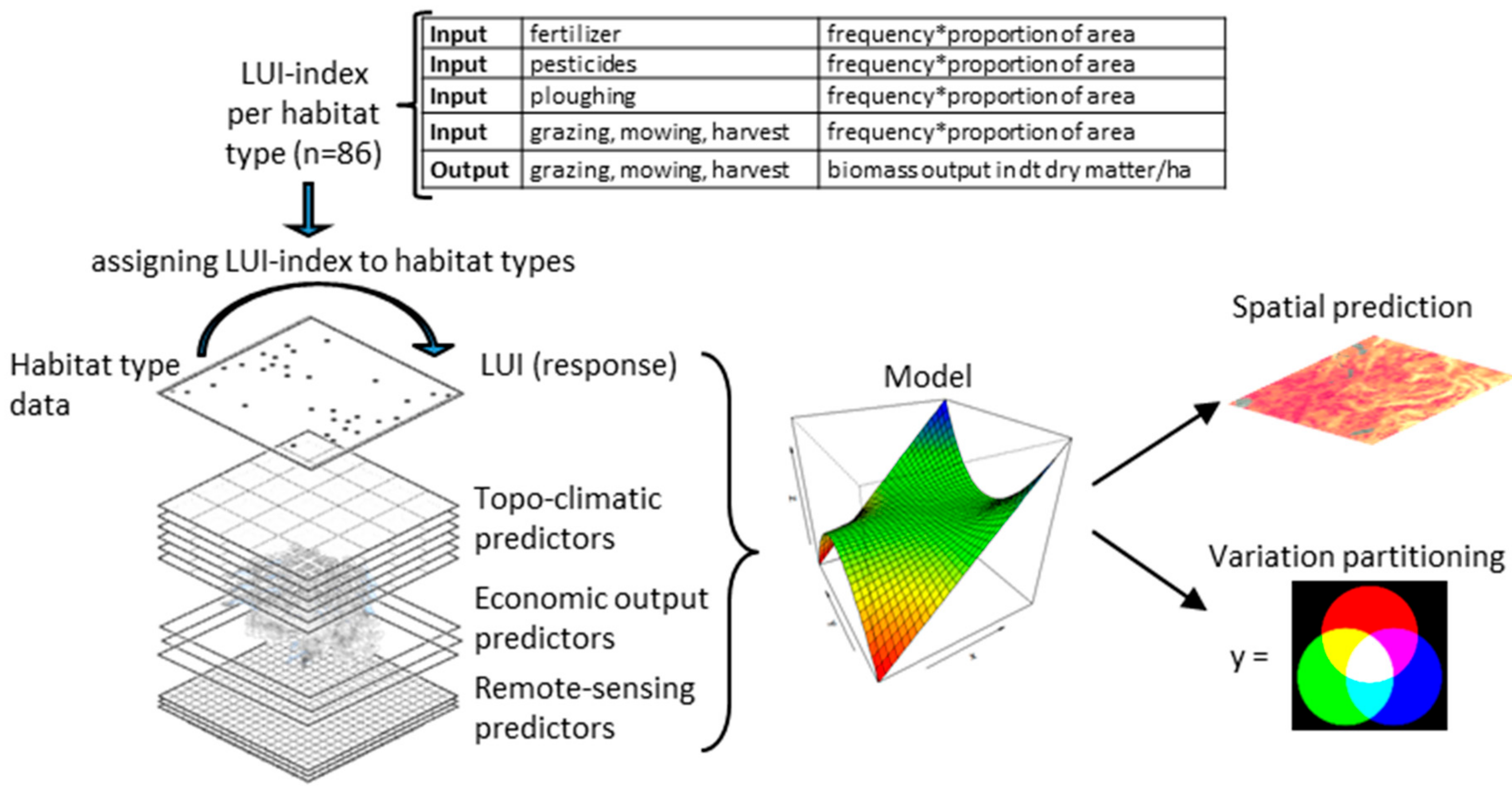
2.1. Framework
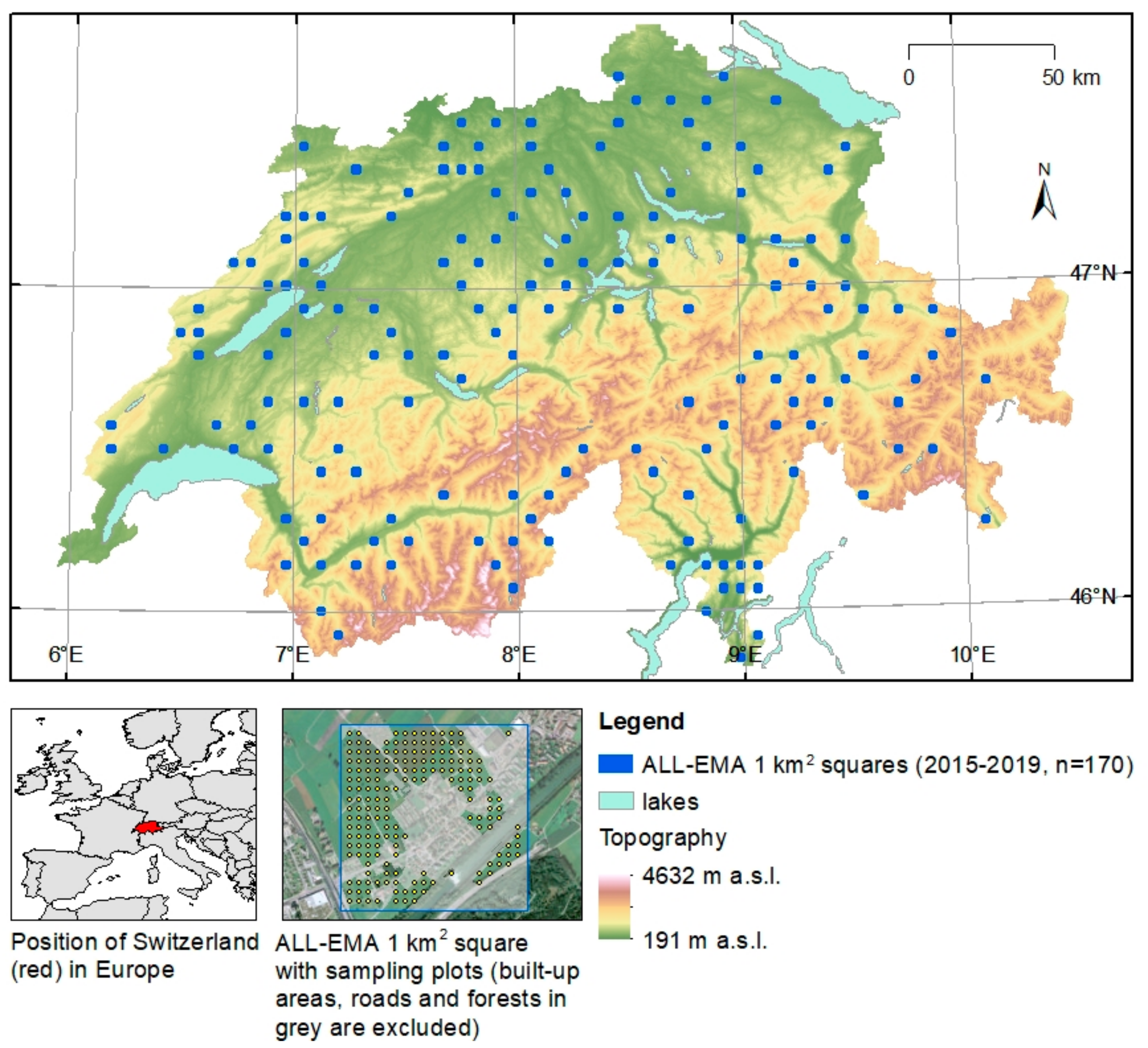
2.2. Study Area
2.3. Data
2.3.1. Habitat Types, Plant Species, and Plant Indicator Values
2.3.2. Topo-Climatic, Economic, and Remote-Sensing Data
2.4. LUI Index per Habitat Type
2.4.1. Parametrisation
2.4.2. Evaluation
2.5. LUI Map and Variation Partitioning
3. Results
3.1. LUI Index Evaluation
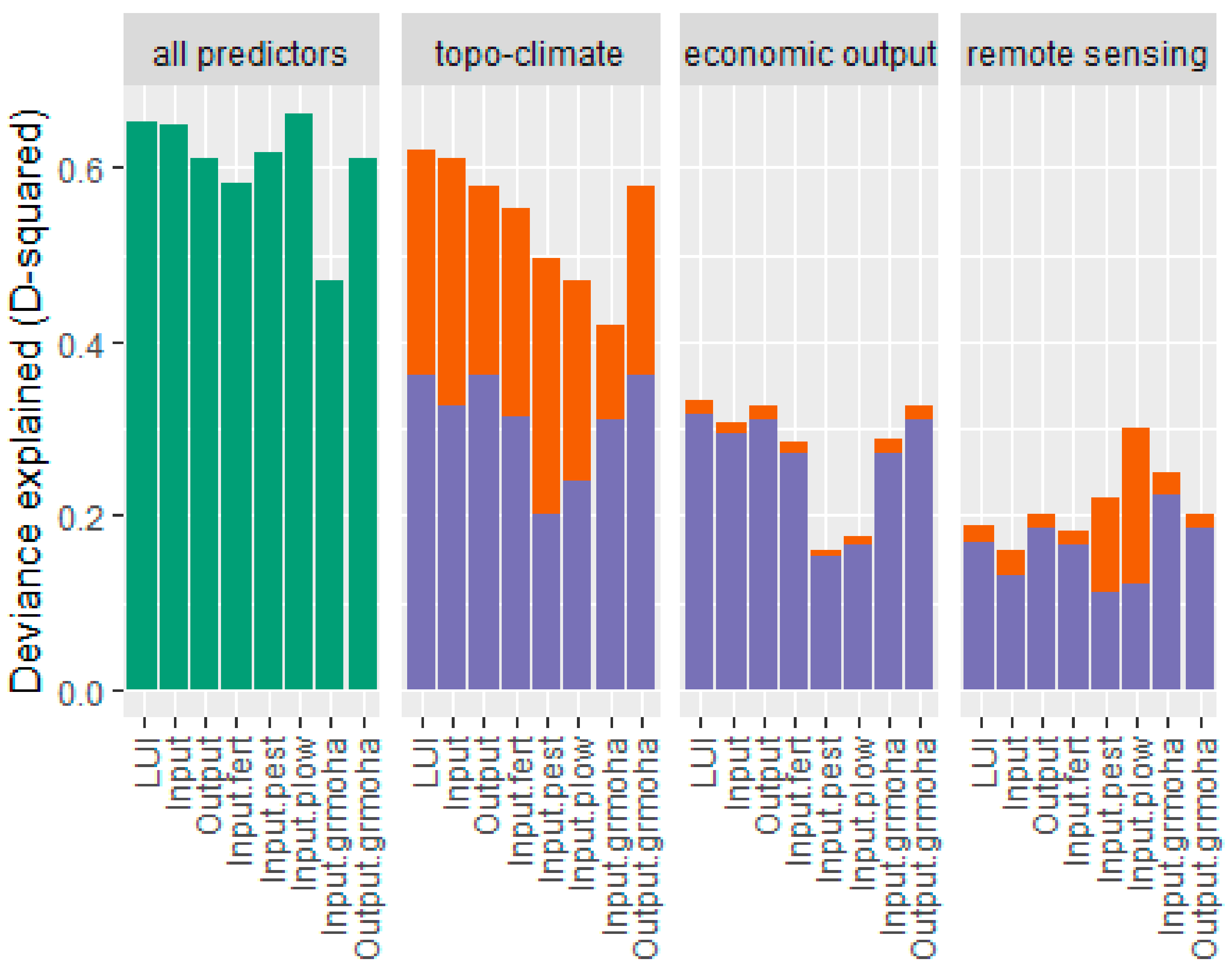
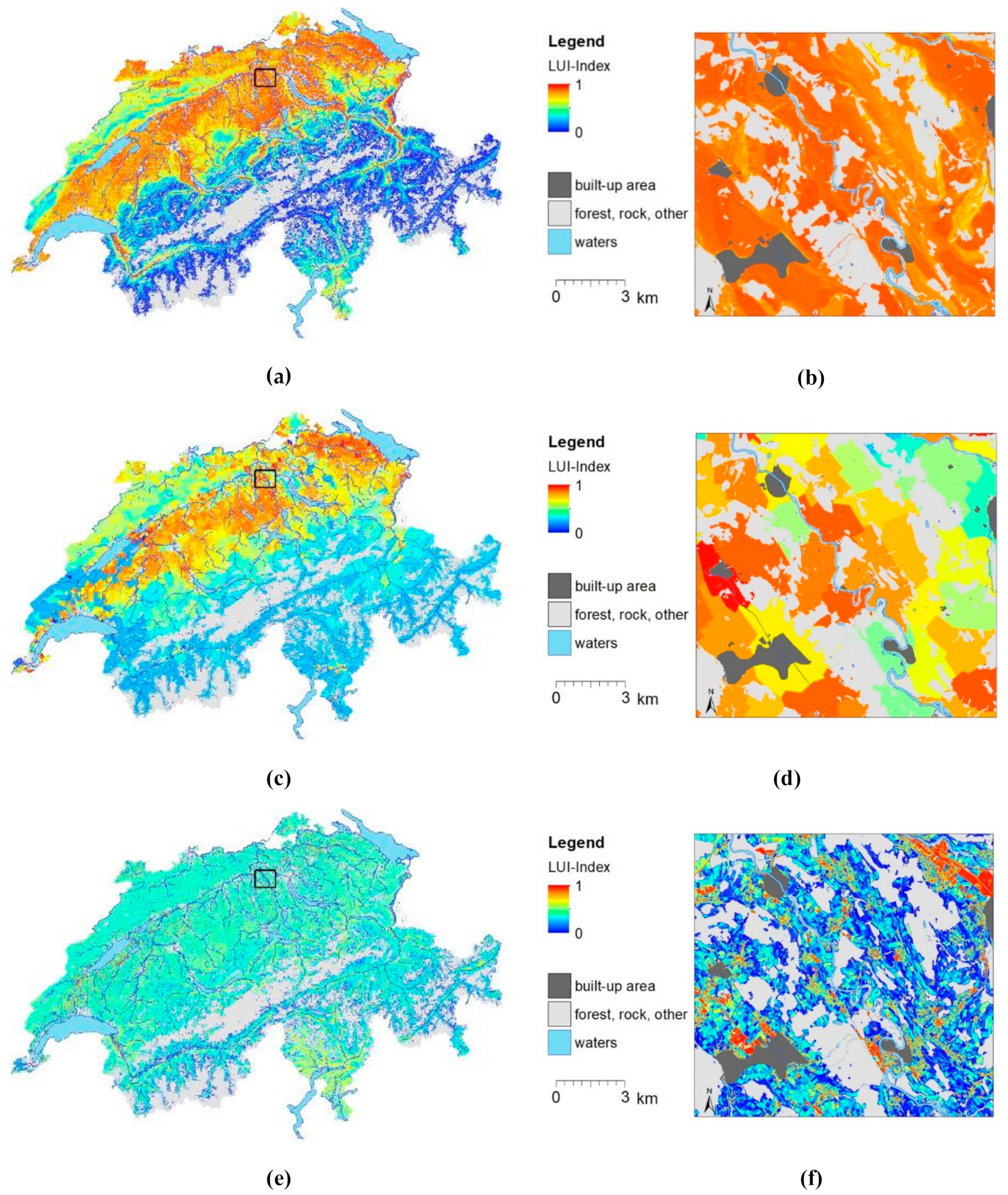
3.2. LUI Map and Variation Partitioning
4. Discussion
4.1. LUI Index Parametrisation and Evaluation
4.2. Spatial Predictions of LUI
4.3. Importance of Biophysical Factors for LUI
4.4. Suitability of Remote-Sensing Data for LUI Mapping
5. Conclusions
Author Contributions
Acknowledgments
Conflicts of Interest
Appendix A

| Habitat Type Code | Habitat Type Name | Fertiliser (Input) | Pesticide (Input) | Ploughing (Input) | Grazing, Mowing, Harvest (Input) | Grazing, Mowing, Harvest (Output) | LUI Index |
|---|---|---|---|---|---|---|---|
| 1 | Non-marine waters | ||||||
| 13 | Springs | ||||||
| 13X | Springs | 0 | 0 | 0 | 0 | 0 | 0 |
| 2 | Vegetation of banks and wetlands | ||||||
| 20 | Artificial banks | ||||||
| 20X | Artificial banks | 0 | 0 | 0 | 0 | 0 | 0 |
| 21 | Water fringe vegetation | ||||||
| 21X | Peatmoss-bladderwort bog pools, Northern perennial amphibious communities, Small reed beds of fast-flowing waters (221, 223, 224) | 0 | 0 | 0 | 0.2 | 1.6 | 0.017 |
| 212 | Reed beds | 0 | 0 | 0 | 0.4 | 3.2 | 0.033 |
| 22 | Fens and transition mires | ||||||
| 221 | Large sedge communities | 0 | 0 | 0 | 0.2 | 0.2 | 0.010 |
| 222 | Acidic fens | 0 | 0 | 0 | 0.5 | 1 | 0.028 |
| 223 | Rich fens | 0 | 0 | 0 | 0.5 | 1 | 0.028 |
| 224 | Transition mires | 0 | 0 | 0 | 0 | 0 | 0.000 |
| 225 | Arcto-alpine riverine swards | 0 | 0 | 0 | 0.2 | 0 | 0.009 |
| 23 | Humid grasslands | ||||||
| 231 | Purple moorgrass meadows and related communities | 0 | 0 | 0 | 0.8 | 8 | 0.073 |
| 232 | Atlantic and Sub-Atlantic humid meadows | 0.5 | 0.1 | 0 | 1.5 | 5 | 0.120 |
| 233 | Meadowsweet stands and related communities | 0.5 | 0 | 0 | 1 | 5 | 0.092 |
| 24 | Raised bogs | ||||||
| 241 | Bog hummocks, ridges, and lawns | 0 | 0 | 0 | 0 | 0 | 0.000 |
| 25 | Temporarily flooded annual vegetation | ||||||
| 25X | Temporarily flooded annual vegetation | 0.1 | 0 | 0 | 0.5 | 0 | 0.028 |
| 3 | Glaciers, rocks, screes, and gravel | ||||||
| 31 | Eternal snow and ice | ||||||
| 314 | Spring snow packs | 0 | 0 | 0 | 0 | 0 | 0 |
| 32 | Alluvial deposits and moraines | ||||||
| 32X | Alluvial deposits and moraines | 0 | 0 | 0 | 0 | 0 | 0.000 |
| 33 | Screes | ||||||
| 33X | Screes | 0 | 0 | 0 | 0 | 0 | 0 |
| 34 | Inland cliffs and exposed rocks | ||||||
| 34X | Inland cliffs and exposed rocks | 0 | 0 | 0 | 0 | 0 | 0 |
| 4 | Grasslands | ||||||
| 40 | Artificial grasslands and lawns | ||||||
| 401 | Temporarily grasslands in rotated crops | 5 | 0.5 | 0.3 | 5 | 110 | 1.000 |
| 403 | Lowland sowings after earthwork (road slopes...) | 0.2 | 0.1 | 0 | 1 | 30 | 0.197 |
| 404 | High altitude sowings after earthwork (ski slopes...) | 0.2 | 0.1 | 0 | 1 | 20 | 0.151 |
| 41 | Rocky flagstones and limestone pavements | ||||||
| 411 | Middle European rock debris swards | 0 | 0 | 0 | 0.1 | 0 | 0.005 |
| 412 | Stepped and garland grasslands | 0 | 0 | 0 | 0 | 0 | 0.000 |
| 413 | Middle European rock debris swards/Pavements | 0 | 0 | 0 | 0.1 | 0 | 0.005 |
| 414 | Alpine weathered rock and outcrop communities/Pavements | 0 | 0 | 0 | 0 | 0 | 0.000 |
| 42 | Thermophilus dry grasslands | ||||||
| 421 | Sub-Continental steppic grasslands | 0 | 0 | 0 | 0.8 | 2 | 0.048 |
| 422 | Sub-Atlantic very dry calcareous grasslands | 0.1 | 0 | 0 | 0.8 | 3 | 0.056 |
| 423 | Insubrian Mesobromion grasslands | 0 | 0 | 0 | 1 | 5 | 0.069 |
| 424 | Sub-Atlantic semi-dry calcareous grasslands | 0.1 | 0.1 | 0 | 2 | 15 | 0.170 |
| 43 | Unfertilised mountain grasslands and pastures | ||||||
| 431 | Blue moorgrass-evergreen sedge slopes | 0 | 0 | 0 | 0.5 | 4 | 0.041 |
| 432 | Cushion sedge carpets | 0 | 0 | 0 | 0.3 | 0 | 0.015 |
| 433 | Northern rusty sedge grasslands | 0 | 0 | 0 | 0.5 | 4 | 0.041 |
| 434 | Wind edge naked-rush swards | 0 | 0 | 0 | 0.2 | 0 | 0.009 |
| 435 | Mat-grass swards and related communities | 0.1 | 0 | 0 | 1 | 8 | 0.087 |
| 436 | Subalpine thermophile siliceous grasslands | 0 | 0 | 0 | 0 | 0 | 0.000 |
| 437 | Crooked-sedge swards and related communities | 0 | 0 | 0 | 0.5 | 1 | 0.025 |
| 44 | Snow-patches | ||||||
| 44X | Snow-patches | 0 | 0 | 0 | 0.1 | 0 | 0.005 |
| 45 | Fertilised grasslands | ||||||
| 451_LD | Medio-European lowland hay meadows (low diversity) | 4 | 0.5 | 0 | 4 | 100 | 0.848 |
| 451_MD | Medio-European lowland hay meadows (medium diversity) | 2 | 0.1 | 0 | 2.5 | 80 | 0.577 |
| 451_HD | Medio-European lowland hay meadows (high diversity) | 0.5 | 0.1 | 0 | 2 | 70 | 0.439 |
| 452_LD | Mountain and subalpine hay meadows (low diversity) | 2 | 0.1 | 0 | 2.7 | 60 | 0.495 |
| 452_MD | Mountain and subalpine hay meadows (medium diversity) | 1.5 | 0.1 | 0 | 1.8 | 35 | 0.316 |
| 452_HD | Mountain and subalpine hay meadows (high diversity) | 1 | 0.1 | 0 | 1.2 | 25 | 0.220 |
| 453_LD | Mesophilic pastures (low diversity) | 3 | 0.2 | 0 | 4 | 100 | 0.788 |
| 453_MD | Mesophilic pastures (medium diversity) | 2 | 0.5 | 0 | 2.5 | 85 | 0.618 |
| 453_HD | Mesophilic pastures (high diversity) | 0.5 | 0.1 | 0 | 1.5 | 50 | 0.324 |
| 454_LD | Rough hawkbit pastures (low diversity) | 0.5 | 0.1 | 0 | 2 | 75 | 0.461 |
| 454_MD | Rough hawkbit pastures (medium diversity) | 0.2 | 0 | 0 | 1 | 35 | 0.215 |
| 454_HD | Rough hawkbit pastures (high diversity) | 0.1 | 0 | 0 | 1 | 25 | 0.165 |
| 46 | Abandoned grasslands | ||||||
| 461 | Abandoned grasslands with Agropyron repens | 0 | 0.2 | 0 | 0.2 | 1 | 0.023 |
| 46X | Abandoned grasslands with Brachypodium pinnatum, Arrhenatherum elatius, Molinia arundinacea, or Calamagrostis varia | 0 | 0.2 | 0 | 0.5 | 2 | 0.041 |
| 5 | Woodland edges, tall herbs communities, scrubs | ||||||
| 51 | Fringes | ||||||
| 511 | Xero-thermophile fringes | 0.2 | 0.1 | 0 | 0.5 | 1 | 0.039 |
| 512 | Mesophilic fringes | 0.2 | 0.1 | 0 | 0.5 | 2 | 0.044 |
| 513 | Mixed riverine screens | 0.1 | 0.1 | 0 | 0.2 | 1 | 0.021 |
| 514 | Butterbur riverine communities | 0 | 0 | 0 | 0.1 | 0 | 0.006 |
| 515 | Shady woodland edge fringes | 0.1 | 0.1 | 0 | 1 | 3 | 0.069 |
| 52 | Clearings | ||||||
| 52X | Burdock and deadly nightshade clearings, Willowherb and foxglove clearings (521, 522) | 0 | 0 | 0 | 0.2 | 0 | 0.010 |
| 523 | Subalpine small reed meadows | 0 | 0 | 0 | 0.2 | 1 | 0.014 |
| 524 | Hercynio-alpine tall herb communities | 0 | 0 | 0 | 0.2 | 0 | 0.011 |
| 525 | Bracken fields | 0.1 | 0.1 | 0 | 0.2 | 2 | 0.026 |
| 53 | Scrubs, brushes, and clearings | ||||||
| 530 | Artificial hedgerows | 0.1 | 0.1 | 0 | 0 | 0 | 0.009 |
| 531 | Medio-European Cytisus scoparius fields | 0 | 0 | 0 | 0.5 | 2 | 0.032 |
| 532 | Blackthorn-privet scrub and box thickets | 0 | 0 | 0 | 0.5 | 1 | 0.028 |
| 533 | Blackthorn-bramble scrub | 0 | 0 | 0 | 0.1 | 0 | 0.006 |
| 534 | Bramble scrubs | 0.1 | 0.1 | 0 | 0.1 | 0 | 0.015 |
| 535 | Shrubby clearings | 0 | 0 | 0 | 0 | 0 | 0.000 |
| 536 | Pre-Alpine Willow brush | 0 | 0 | 0 | 0.5 | 0 | 0.023 |
| 537 | Mire Willow scrub | 0 | 0 | 0 | 0 | 0 | 0.000 |
| 538 | Willow brush | 0 | 0 | 0 | 0.1 | 0 | 0.005 |
| 539 | Alpine green alder scrub | 0 | 0 | 0 | 0.1 | 0 | 0.005 |
| 54 | Dry heaths | ||||||
| 541 | Sub-Atlantic acidophilous heaths | 0 | 0 | 0 | 0.5 | 1 | 0.025 |
| 542 | Juniperus sabina scrub | 0 | 0 | 0 | 0.2 | 0 | 0.010 |
| 543 | Bearberry and hairy alpenrose heaths | 0 | 0 | 0 | 0 | 0 | 0.000 |
| 544 | Juniperus nana scrub | 0 | 0 | 0 | 0.5 | 1 | 0.025 |
| 545 | Alpenrose heaths | 0 | 0 | 0 | 0.5 | 1 | 0.025 |
| 546 | Dwarf Azalea and Vaccinium heaths | 0 | 0 | 0 | 0.1 | 0 | 0.005 |
| 6 | Forests | ||||||
| 6X | Forests | ||||||
| 6XX | Forests | 0 | 0 | 0 | 0.5 | 1 | 0.028 |
| 7 | Pioneer vegetation of disturbed areas (ruderal vegetation) | ||||||
| 71 | Trampled and ruderal areas | ||||||
| 710 | Trampled ground and unvegetated ruins or debris | 1 | 0.1 | 0.1 | 0 | 0 | 0.056 |
| 711 | Flood swards and related communities | 1 | 0.1 | 0.1 | 3 | 2 | 0.204 |
| 712 | Lowland fallow fields | 1 | 0.1 | 0.1 | 3 | 2 | 0.204 |
| 713 | Subalpine and Alpine fallow fields | 1 | 0 | 0 | 2 | 30 | 0.275 |
| 714 | Annual ruderal vegetation | 0.2 | 0.1 | 0.5 | 0 | 0 | 0.037 |
| 715 | Pluriannual thermophilus ruderal vegetation | 0.1 | 0 | 0.2 | 0.2 | 0 | 0.025 |
| 716 | Pluriannual mesophilic ruderal vegetation | 0.1 | 0.1 | 0.2 | 0 | 0 | 0.019 |
| 717 | Alpine dock communities | 1 | 0.1 | 0 | 1 | 10 | 0.143 |
| 718 | Lowland dock communities | 0.1 | 0 | 0.1 | 0.2 | 0 | 0.020 |
| 72 | Anthropogenic rocky habitats | ||||||
| 720 | Unvegetated walls or paved areas | 0 | 0.2 | 0 | 0 | 0 | 0.009 |
| 721 | Vegetated ruins or old walls | 0 | 0.1 | 0 | 0 | 0 | 0.005 |
| 722 | Vegetated paved areas | 0 | 1 | 0 | 0 | 0 | 0.046 |
| 8 | Plantations, fields, and cropland | ||||||
| 81 | Cultivated ligneous formations | ||||||
| 81X | Deciduous seedbeds, Coniferous seedbeds, Chestnut groves (without undergrowth), High stem orchard | 0.1 | 4 | 0.1 | 1.1 | 5 | 0.268 |
| 815 | Low-stem orchard | 2 | 5 | 0.2 | 1.1 | 5 | 0.407 |
| 816 | Vineyards | 2 | 5 | 0.3 | 0.6 | 2 | 0.377 |
| 817 | Small fruits | 3 | 3 | 0.5 | 0.5 | 3 | 0.335 |
| 82 | Field crops | ||||||
| 82X_LD | Field crops (low diversity) | 3 | 3 | 1.5 | 2 | 100 | 0.894 |
| 82X_MD | Field crops (medium diversity) | 2 | 2 | 1.5 | 2 | 100 | 0.802 |
| 82X_HD | Field crops (high diversity) | 1.5 | 1.5 | 1.5 | 1.5 | 100 | 0.732 |
References
- Godfray, H.C.J.; Beddington, J.R.; Crute, I.R.; Haddad, L.; Lawrence, D.; Muir, J.F.; Pretty, J.; Robinson, S.; Thomas, S.M.; Toulmin, C. Food security: The challenge of feeding 9 billion people. Science 2010, 327, 812–818. [Google Scholar] [CrossRef] [PubMed] [Green Version]
- Meehan, T.D.; Werling, B.P.; Landis, D.A.; Gratton, C. Agricultural landscape simplification and insecticide use in the Midwestern United States. Proc. Natl. Acad. Sci. USA 2011, 108, 11500–11505. [Google Scholar] [CrossRef] [Green Version]
- Pe’er, G.; Dicks, L.V.; Visconti, P.; Arlettaz, R.; Báldi, A.; Benton, T.G.; Collins, S.; Dieterich, M.; Gregory, R.D.; Hartig, F.; et al. EU agricultural reform fails on biodiversity. Science 2014, 344, 1090–1092. [Google Scholar] [CrossRef] [PubMed]
- Titeux, N.; Henle, K.; Mihoub, J.-B.; Brotons, L. Climate change distracts us from equally important threats to biodiversity. Front. Ecol. Environ. 2016, 14, 291. [Google Scholar] [CrossRef]
- Newbold, T.; Hudson, L.N.; Hill, S.L.L.; Contu, S.; Lysenko, I.; Senior, R.A.; Borger, L.; Bennett, D.J.; Choimes, A.; Collen, B.; et al. Global effects of land use on local terrestrial biodiversity. Nature 2015, 520, 45–50. [Google Scholar] [CrossRef] [Green Version]
- Fahrig, L. Rethinking patch size and isolation effects: The habitat amount hypothesis. J. Biogeogr. 2013, 40, 1649–1663. [Google Scholar] [CrossRef]
- Gerstner, K.; Dormann, C.F.; Stein, A.; Manceur, A.M.; Seppelt, R. Effects of land use on plant diversity—A global meta-analysis. J. Appl. Ecol. 2014, 51, 1690–1700. [Google Scholar] [CrossRef]
- Seppelt, R.; Beckmann, M.; Ceauşu, S.; Cord, A.F.; Gerstner, K.; Gurevitch, J.; Kambach, S.; Klotz, S.; Mendenhall, C.; Phillips, H.R.P.; et al. Harmonizing biodiversity conservation and productivity in the context of increasing demands on landscapes. Bioscience 2016, 66, 890–896. [Google Scholar] [CrossRef]
- Foley, J.A.; Ramankutty, N.; Brauman, K.A.; Cassidy, E.S.; Gerber, J.S.; Johnston, M.; Mueller, N.D.; O’Connell, C.; Ray, D.K.; West, P.C.; et al. Solutions for a cultivated planet. Nature 2011, 478, 337–342. [Google Scholar] [CrossRef] [Green Version]
- MacDonald, D.; Crabtree, J.R.; Wiesinger, G.; Dax, T.; Stamou, N.; Fleury, P.; Gutierrez Lazpita, J.; Gibon, A. Agricultural abandonment in mountain areas of Europe: Environmental consequences and policy response. J. Environ. Manag. 2000, 59, 47–69. [Google Scholar] [CrossRef]
- Stoate, C.; Boatman, N.D.; Borralho, R.J.; Carvalho, C.R.; De Snoo, G.R.; Eden, P. Ecological impacts of arable intensification in Europe. J. Environ. Manag. 2001, 63, 337–365. [Google Scholar] [CrossRef] [PubMed]
- Benton, T.G.; Vickery, J.A.; Wilson, J.D. Farmland biodiversity: Is habitat heterogeneity the key? Trends Ecol. Evol. 2003, 18, 182–188. [Google Scholar] [CrossRef]
- Pereira, H.M.; Navarro, L.M.; Martins, I.S. Global Biodiversity Change: The Bad, the Good, and the Unknown. Annu. Rev. Environ. Resour. 2012, 37, 25–50. [Google Scholar] [CrossRef] [Green Version]
- Tasser, E.; Walde, J.; Tappeiner, U.; Teutsch, A.; Noggler, W. Land-use changes and natural reforestation in the Eastern Central Alps. Agric. Ecosyst. Environ. 2007, 118, 115–129. [Google Scholar] [CrossRef]
- Kolecka, N.; Kozak, J.; Kaim, D.; Dobosz, M.; Ginzler, C.; Psomas, A. Mapping secondary forest succession on abandoned agricultural land with LiDAR point clouds and terrestrial photography. Remote Sens. 2015, 7, 8300–8322. [Google Scholar] [CrossRef] [Green Version]
- Kuemmerle, T.; Erb, K.; Meyfroidt, P.; Müller, D.; Verburg, P.H.; Estel, S.; Haberl, H.; Hostert, P.; Jepsen, M.R.; Kastner, T.; et al. Challenges and opportunities in mapping land use intensity globally. Curr. Opin. Environ. Sustain. 2013, 5, 484–493. [Google Scholar] [CrossRef]
- De Chazal, J.; Rounsevell, M.D.A. Land-use and climate change within assessments of biodiversity change: A review. Glob. Environ. Chang. 2009, 19, 306–315. [Google Scholar] [CrossRef]
- Stürck, J.; Levers, C.; Van der Zanden, E.H.; Schulp, C.J.E.; Verkerk, P.J.; Kuemmerle, T.; Helming, J.; Lotze-Campen, H.; Tabeau, A.; Popp, A.; et al. Simulating and delineating future land change trajectories across Europe. Reg. Environ. Chang. 2018, 18, 733–749. [Google Scholar] [CrossRef] [Green Version]
- Moser, D.; Dullinger, S.; Mang, T.; Hülber, K.; Essl, F.; Frank, T.; Hulme, P.E.; Grabherr, G.; Pascher, K. Changes in plant life-form, pollination syndrome and breeding system at a regional scale promoted by land use intensity. Divers. Distrib. 2015, 21, 1319–1328. [Google Scholar] [CrossRef]
- Rüdisser, J.; Tasser, E.; Tappeiner, U. Distance to nature—A new biodiversity relevant environmental indicator set at the landscape level. Ecol. Indic. 2012, 15, 208–216. [Google Scholar] [CrossRef]
- Rüdisser, J.; Walde, J.; Tasser, E.; Frühauf, J.; Teufelbauer, N.; Tappeiner, U. Biodiversity in cultural landscapes: Influence of land use intensity on bird assemblages. Landsc. Ecol. 2015, 30, 1851–1863. [Google Scholar] [CrossRef]
- Kovács-Hostyánszki, A.; Földesi, R.; Mózes, E.; Szirák, Á.; Fischer, J.; Hanspach, J.; Báldi, A. Conservation of pollinators in traditional agricultural landscapes—New challenges in Transylvania (Romania) posed by EU accession and recommendations for future research. PLoS ONE 2016, 11, e0151650. [Google Scholar] [CrossRef] [PubMed] [Green Version]
- Herzog, F.; Steiner, B.; Bailey, D.; Baudry, J.; Billeter, R.; Bukácek, R.; De Blust, G.; De Cock, R.; Dirksen, J.; Dormann, C.F.; et al. Assessing the intensity of temperate European agriculture at the landscape scale. Eur. J. Agron. 2006, 24, 165–181. [Google Scholar] [CrossRef]
- Tuck, S.L.; Winqvist, C.; Mota, F.; Ahnström, J.; Turnbull, L.A.; Bengtsson, J. Land-use intensity and the effects of organic farming on biodiversity: A hierarchical meta-analysis. J. Appl. Ecol. 2014, 51, 746–755. [Google Scholar] [CrossRef]
- Rhodes, C.J.; Henrys, P.; Siriwardena, G.M.; Whittingham, M.J.; Norton, L.R. The relative value of field survey and remote sensing for biodiversity assessment. Methods Ecol. Evol. 2015, 6, 772–781. [Google Scholar] [CrossRef]
- Pereira, H.M.; Daily, G.C. Modeling biodiversity dynamics in countryside landscapes. Ecology 2006, 87, 1877–1885. [Google Scholar] [CrossRef]
- Koh, L.P.; Ghazoul, J. A matrix-calibrated species-area model for predicting biodiversity losses due to land-use change. Conserv. Biol. 2010, 24, 994–1001. [Google Scholar] [CrossRef]
- Prugh, L.R.; Hodges, K.E.; Sinclair, A.R.E.; Brashares, J.S. Effect of habitat area and isolation on fragmented animal populations. Proc. Natl. Acad. Sci. USA 2008, 105, 20770–20775. [Google Scholar] [CrossRef] [Green Version]
- Revilla, E.; Wiegand, T.; Palomares, F.; Ferreras, P.; Delibes, M. Effects of matrix heterogeneity on animal dispersal: From individual behavior to metapopulation-level parameters. Am. Nat. 2004, 164, E130–E153. [Google Scholar] [CrossRef] [Green Version]
- Bender, D.J.; Fahrig, L. Matrix structure obscures the relationship between interpatch movement and patch size and isolation. Ecology 2005, 86, 1023–1033. [Google Scholar] [CrossRef] [Green Version]
- Tubelis, D.P.; Lindenmayer, D.B.; Cowling, A. Bird populations in native forest patches in south-eastern Australia: The roles of patch width, matrix type (age) and matrix use. Landsc. Ecol. 2007, 22, 1045–1058. [Google Scholar] [CrossRef]
- Harfoot, M.B.J.J.; Newbold, T.; Tittensor, D.P.; Emmott, S.; Hutton, J.; Lyutsarev, V.; Smith, M.J.; Scharlemann, J.P.W.W.; Purves, D.W. Emergent global patterns of ecosystem structure and function from a mechanistic general ecosystem model. PLoS Biol. 2014, 12, 1–24. [Google Scholar] [CrossRef] [PubMed] [Green Version]
- Erb, K.-H.; Haberl, H.; Jepsen, M.R.; Kuemmerle, T.; Lindner, M.; Müller, D.; Verburg, P.H.; Reenberg, A. A conceptual framework for analysing and measuring land-use intensity. Curr. Opin. Environ. Sustain. 2013, 5, 464–470. [Google Scholar] [CrossRef] [Green Version]
- Busch, V.; Klaus, V.H.; Schäfer, D.; Prati, D.; Boch, S.; Müller, J.; Chisté, M.; Mody, K.; Blüthgen, N.; Fischer, M.; et al. Will I stay or will I go? Plant species-specific response and tolerance to high land-use intensity in temperate grassland ecosystems. J. Veg. Sci. 2019, 30, 674–686. [Google Scholar] [CrossRef]
- Estel, S.; Kuemmerle, T.; Levers, C.; Baumann, M.; Hostert, P. Mapping cropland-use intensity across Europe using MODIS NDVI time series. Environ. Res. Lett. 2016, 11, 024015. [Google Scholar] [CrossRef] [Green Version]
- Gómez Giménez, M.; De Jong, R.; Della Peruta, R.; Keller, A.; Schaepman, M.E. Determination of grassland use intensity based on multi-temporal remote sensing data and ecological indicators. Remote Sens. Environ. 2017, 198, 126–139. [Google Scholar] [CrossRef]
- Estel, S.; Kuemmerle, T.; Alcántara, C.; Levers, C.; Prishchepov, A.; Hostert, P. Mapping farmland abandonment and recultivation across Europe using MODIS NDVI time series. Remote Sens. Environ. 2015, 163, 312–325. [Google Scholar] [CrossRef]
- Griffiths, P.; Nendel, C.; Pickert, J.; Hostert, P. Towards national-scale characterization of grassland use intensity from integrated Sentinel-2 and Landsat time series. Remote Sens. Environ. 2020, 238, 111124. [Google Scholar] [CrossRef]
- Kolecka, N.; Ginzler, C.; Pazur, R.; Price, B.; Verburg, P.H. Regional scale mapping of grassland mowing frequency with Sentinel-2 time series. Remote Sens. 2018, 10, 1221. [Google Scholar] [CrossRef] [Green Version]
- Veloso, A.; Mermoz, S.; Bouvet, A.; Le Toan, T.; Planells, M.; Dejoux, J.F.; Ceschia, E. Understanding the temporal behavior of crops using Sentinel-1 and Sentinel-2-like data for agricultural applications. Remote Sens. Environ. 2017, 199, 415–426. [Google Scholar] [CrossRef]
- Denize, J.; Hubert-Moy, L.; Betbeder, J.; Corgne, S.; Baudry, J.; Pottier, E. Evaluation of using sentinel-1 and -2 time-series to identify winter land use in agricultural landscapes. Remote Sens. 2019, 11, 37. [Google Scholar] [CrossRef] [Green Version]
- Howison, R.A.; Piersma, T.; Kentie, R.; Hooijmeijer, J.C.E.W.; Olff, H. Quantifying landscape-level land-use intensity patterns through radar-based remote sensing. J. Appl. Ecol. 2018, 55, 1276–1287. [Google Scholar] [CrossRef] [Green Version]
- Verburg, P.H.; Overmars, K.P. Combining top-down and bottom-up dynamics in land use modeling: Exploring the future of abandoned farmlands in Europe with the Dyna-CLUE model. Landsc. Ecol. 2009, 24, 1167. [Google Scholar] [CrossRef]
- Allan, E.; Manning, P.; Alt, F.; Binkenstein, J.; Blaser, S.; Blüthgen, N.; Böhm, S.; Grassein, F.; Hölzel, N.; Klaus, V.H.; et al. Land use intensification alters ecosystem multifunctionality via loss of biodiversity and changes to functional composition. Ecol. Lett. 2015, 18, 834–843. [Google Scholar] [CrossRef]
- Allan, E.; Bossdorf, O.; Dormann, C.F.; Prati, D.; Gossner, M.M.; Tscharntke, T.; Bluthgen, N.; Bellach, M.; Birkhofer, K.; Boch, S.; et al. Interannual variation in land-use intensity enhances grassland multidiversity. Proc. Natl. Acad. Sci. USA 2014, 111, 308–313. [Google Scholar] [CrossRef] [Green Version]
- Bernhardt-Römermann, M.; Römermann, C.; Sperlich, S.; Schmidt, W. Explaining grassland biomass—The contribution of climate, species and functional diversity depends on fertilization and mowing frequency. J. Appl. Ecol. 2011, 48, 1088–1097. [Google Scholar] [CrossRef] [Green Version]
- Landolt, E.; Bäumler, B.; Erhardt, A.; Hegg, O.; Klötzli, F.; Lämmler, W.; Nobis, M.; Rudmann-Maurer, K.; Schweingruber, F.H.; Theurillat, J.P. Flora Indicativa—Ökologische Zeigerwerte und Biologische Kennzeichen zur Flora der Schweiz und der Alpen; Haupt: Bern, Switzerland, 2010. [Google Scholar]
- Braun-Blanquet, J. Pflanzensoziologie, Grundzüge der Vegetationskunde; Springer: Wien, Austria, 1964. [Google Scholar]
- Naimi, B.; Araújo, M.B. Sdm: A reproducible and extensible R platform for species distribution modelling. Ecography 2016, 39, 368–375. [Google Scholar] [CrossRef] [Green Version]
- Neter, J.; Wasserman, W.; Kutner, M. Applied Linear Regression Models; Irwin, Inc.: Homewood, IL, USA, 1983. [Google Scholar]
- Chatterjee, S.; Hadi, A.S. Regression Analysis by Example; John Wiley & Sons: Hoboken, NJ, USA, 2006. [Google Scholar]
- R Core Team. R: A language and environment for statistical computing. R Foundation for Statistical Computing, Vienna, Austria. Available online: https://www.R-project.org/ (accessed on 1 July 2019).
- ESRI. ArcGIS Desctop: Release 10.7.1; Environmental Systems Research Institute: Redlands, CA, USA, 2019. [Google Scholar]
- Swisstopo. DHM25—Das Digitale Hoehenmodell der Schweiz [DHM25—Digital Terrain Model of Switzerland]. 2005. Available online: https://shop.swisstopo.admin.ch/en/products/height_models/dhm25 (accessed on 30 January 2019).
- Hijmans, R.J.; Cameron, S.E.; Parra, J.L.; Jones, P.G.; Jarvis, A. Very high resolution interpolated climate surfaces for global land areas. Int. J. Climatol. 2005, 25, 1965–1978. [Google Scholar] [CrossRef]
- Zimmermann, N.E.; Kienast, F. Predictive mapping of alpine grasslands in Switzerland: Species versus community approach. J. Veg. Sci. 1999, 10, 469–482. [Google Scholar] [CrossRef]
- Guisan, A.; Zimmermann, N.E.N.E.; Elith, J.; Graham, C.H.; Phillips, S.; Peterson, A.T. What matters for predicting the occurrences of trees: Techniques, data, or species’ characteristics? Ecol. Monogr. 2007, 77, 615–630. [Google Scholar] [CrossRef] [Green Version]
- BFS and BLW. BEK200: Bodeneignungskarte der Schweiz 1:200′000 [BEK200: Soil suitability map of Switzerland]. 2000. Available online: https://www.blw.admin.ch/blw/de/home/politik/datenmanagement/geografisches-informationssystem-gis/download-geodaten.html (accessed on 30 January 2019).
- BLW. Agrarpolitisches Informationssystem AGIS. Available online: https://www.blw.admin.ch/blw/de/home/politik/datenmanagement/agate/agis.html (accessed on 30 January 2019).
- Alcaraz-Segura, D.; Lomba, A.; Sousa-Silva, R.; Nieto-Lugilde, D.; Alves, P.; Georges, D.; Vicente, J.R.; Honrado, J.P. Potential of satellite-derived ecosystem functional attributes to anticipate species range shifts. Int. J. Appl. Earth Obs. Geoinf. 2017, 57, 86–92. [Google Scholar] [CrossRef]
- Pettorelli, N.; Vik, J.O.; Mysterud, A.; Gaillard, J.M.; Tucker, C.J.; Stenseth, N.C. Using the satellite-derived NDVI to assess ecological responses to environmental change. Trends Ecol. Evol. 2005, 20, 503–510. [Google Scholar] [CrossRef] [PubMed]
- Pettorelli, N.; Wegmann, M.; Skidmore, A.; Mücher, S.; Dawson, T.P.; Fernandez, M.; Lucas, R.; Schaepman, M.E.; Wang, T.; O’Connor, B.; et al. Framing the concept of satellite remote sensing essential biodiversity variables: Challenges and future directions. Remote Sens. Ecol. Conserv. 2016, 2, 122–131. [Google Scholar] [CrossRef]
- Rihm, B.; Achermann, B. Critical loads of nitrogen and their exceedances. Swiss contribution to the effects-oriented work under the convention on long-range transboundary air pollution (UNECE). FOEN Environ. Stud. 2016, 1642, 78. [Google Scholar]
- Thornton, P.E.; Running, S.W.; White, M.A. Generating surfaces of daily meteorological variables over large regions of complex terrain. J. Hydrol. 1997, 190, 214–251. [Google Scholar] [CrossRef] [Green Version]
- Delarze, R.; Gonseth, Y. Lebensräume der Schweiz: Ökologie, Gefährdung, Kennarten; Ott Verlag: Thun, Switzerland, 2008; Volume 2. [Google Scholar]
- Blüthgen, N.; Dormann, C.F.; Prati, D.; Klaus, V.H.; Kleinebecker, T.; Hölzel, N.; Alt, F.; Boch, S.; Gockel, S.; Hemp, A.; et al. A quantitative index of land-use intensity in grasslands: Integrating mowing, grazing and fertilization. Basic Appl. Ecol. 2012, 13, 207–220. [Google Scholar] [CrossRef]
- Weisberg, S. Applied Linear Regression; Wiley: New York, NY, USA, 1980; ISBN 0-471-04419-9. [Google Scholar]
- Guisan, A.; Zimmermann, N.E. Predictive habitat distribution models in ecology. Ecol. Modell. 2000, 135, 147–186. [Google Scholar] [CrossRef]
- Zhang, D. A coefficient of determination for generalized linear models. Am. Stat. 2017, 71, 310–316. [Google Scholar] [CrossRef]
- Voltz, M.; Webster, R. A comparison of kriging, cubic splines and classification for predicting soil properties from sample information. J. Soil Sci. 1990, 41, 473–490. [Google Scholar] [CrossRef]
- Venables, W.N.; Ripley, B.D.; William, N.V. Modern Applied Statistics with S-Plus; Springer: New York, NY, USA, 2002. [Google Scholar]
- Borcard, D.; Legendre, P.; Drapeau, P. Partialling out the spatial component of ecological variation. Ecology 1992, 73, 1045–1055. [Google Scholar] [CrossRef] [Green Version]
- Real, R.; Barbosa, A.M.; Porras, D.; Kin, M.S.; Márquez, A.L.; Guerrero, J.C.; Palomo, L.J.; Justo, E.R.; Vargas, J.M. Relative importance of environment, human activity and spatial situation in determining the distribution of terrestrial mammal diversity in Argentina. J. Biogeogr. 2003, 30, 939–947. [Google Scholar] [CrossRef]
- Blüthgen, N.; Simons, N.K.; Jung, K.; Prati, D.; Renner, S.C.; Boch, S.; Fischer, M.; Hölzel, N.; Klaus, V.H.; Kleinebecker, T.; et al. Land use imperils plant and animal community stability through changes in asynchrony rather than diversity. Nat. Commun. 2016, 7, 1–7. [Google Scholar] [CrossRef] [PubMed] [Green Version]
- Verburg, P.H.; Crossman, N.; Ellis, E.C.; Heinimann, A.; Hostert, P.; Mertz, O.; Nagendra, H.; Sikor, T.; Erb, K.H.; Golubiewski, N.; et al. Land system science and sustainable development of the earth system: A global land project perspective. Anthropocene 2015, 12, 29–41. [Google Scholar] [CrossRef] [Green Version]
- Holzkämper, A.; Fossati, D.; Hiltbrunner, J.; Fuhrer, J. Spatial and temporal trends in agro-climatic limitations to production potentials for grain maize and winter wheat in Switzerland. Reg. Environ. Chang. 2014, 15, 109–122. [Google Scholar] [CrossRef]
- Tuanmu, M.N.; Jetz, W. A global, remote sensing-based characterization of terrestrial habitat heterogeneity for biodiversity and ecosystem modelling. Glob. Ecol. Biogeogr. 2015, 24, 1329–1339. [Google Scholar] [CrossRef]
- Skowronek, S.; Ewald, M.; Isermann, M.; Van De Kerchove, R.; Lenoir, J.; Aerts, R.; Warrie, J.; Hattab, T.; Honnay, O.; Schmidtlein, S.; et al. Mapping an invasive bryophyte species using hyperspectral remote sensing data. Biol. Invasions 2017, 19, 239–254. [Google Scholar] [CrossRef]
- Lausch, A.; Bannehr, L.; Beckmann, M.; Boehm, C.; Feilhauer, H.; Hacker, J.M.; Heurich, M.; Jung, A.; Klenke, R.; Neumann, C.; et al. Linking Earth Observation and taxonomic, structural and functional biodiversity: Local to ecosystem perspectives. Indic. Ecol. 2016, 70, 317–339. [Google Scholar] [CrossRef]
- Rocchini, D.; Luque, S.; Pettorelli, N.; Bastin, L.; Doktor, D.; Faedi, N.; Feilhauer, H.; Féret, J.B.; Foody, G.M.; Gavish, Y.; et al. Measuring β-diversity by remote sensing: A challenge for biodiversity monitoring. Methods Ecol. Evol. 2018, 9, 1787–1798. [Google Scholar] [CrossRef] [Green Version]
- Siebert, S.; Portmann, F.T.; Döll, P. Global patterns of cropland use intensity. Remote Sens. 2010, 2, 1625–1643. [Google Scholar] [CrossRef] [Green Version]
- He, K.S.; Bradley, B.A.; Cord, A.F.; Rocchini, D.; Tuanmu, M.N.; Schmidtlein, S.; Turner, W.; Wegmann, M.; Pettorelli, N. Will remote sensing shape the next generation of species distribution models? Remote Sens. Ecol. Conserv. 2015, 1, 4–18. [Google Scholar] [CrossRef] [Green Version]
- Zimmermann, N.E.; Edwards, T.C.; Moisen, G.G.; Frescino, T.S.; Blackard, J.A. Remote sensing-based predictors improve distribution models of rare, early successional and broadleaf tree species in Utah. J. Appl. Ecol. 2007, 44, 1057–1067. [Google Scholar] [CrossRef] [PubMed] [Green Version]
- Fahrig, L. Effects of habitat fragmentation on biodiversity. Annu. Rev. Ecol. Evol. Syst. 2003, 34, 487–515. [Google Scholar] [CrossRef] [Green Version]

| Predictor Set | Variable Name/Description | Range (min, max) | Unit | Source |
|---|---|---|---|---|
| Topo-climatic | Degree-days with a 0 °C threshold | 0–45,832 | °C d | Wordclim data of 1950–2000 [55] downscaled with Daymet following Thornton et al. [64] according to Zimmermann and Kienast [56]. |
| Topo-climatic | Yearly precipitation days | 20–59 | d | Wordclim data of 1950–2000 [55] downscaled with Daymet following Thornton et al. [64] according to Zimmermann and Kienast [56]. |
| Topo-climatic | Slope | 0–88 | ° | Calculated with ArcGIS from DHM25 [54]. |
| Topo-climatic | Potential yearly global radiation | 2,180–23,443 | kJ m−2 d−1 | Calculated according to Zimmermann and Kienast [56] from DHM25 [54]. |
| Topo-climatic | Topographic position index | 616–1589 | m | Calculated according to Zimmermann and Kienast [56] from DHM25 [54]. |
| Topo-climatic | Summer frost days | 0–8,8154 | d | Wordclim data of 1950–2000 [55] downscaled with Daymet following Thornton et al. [64] according to Zimmermann and Kienast [56]. |
| Topo-climatic | Soil suitability for agricultural land-use | 1–18 | - | Soil suitability map of Switzerland [58]. |
| Remote sensing | Mean NDVI | −1–1 | - | Sentinel-2 (ESA) |
| Remote sensing | SD NDVI | 0–0.3 | - | Sentinel-2 (ESA) |
| Economic output | Agricultural standard output coefficient of cattle, sheep, and goats (AGIS-codes 1110–1586 and 1882) | 0–79,603 | CHF km−2 | AGIS database for the years 2005–2009 [59]. |
| Economic output | Agricultural standard output coefficient of pigs and poultry (AGIS-codes 1611–1881) | 0–38,202 | CHF km−2 | AGIS database for the years 2005–2009 [59]. |
| Economic output | Agricultural standard output coefficient crop area (AGIS-codes 501–598) | 0–114,802 | CHF km−2 | AGIS database for the years 2005–2009 [59]. |
| Economic output | Agricultural standard output coefficient of permanent crops (AGIS-codes 701–798) | 0–184,619 | CHF km−2 | AGIS database for the years 2005–2009 [59]. |
| Economic output | Agricultural standard output coefficient of protected crops (AGIS-codes 801–898) | 0–178,432 | CHF km−2 | AGIS database for the years 2005–2009 [59]. |
| Aerial nitrogen deposition | Aerial nitrogen deposition (critical loads) | 2–50 | kg ha−1 y−1 | Rihm and Achermann [63]. |
| Dimension of LUI | LUI Factors | Rating |
|---|---|---|
| Input | Fertiliser | frequency*proportion of areaa |
| Input | Pesticide | frequency*proportion of areaa |
| Input | Ploughing | frequency*proportion of areaa |
| Input | Grazing, mowing, harvesting | frequency*proportion of areaa |
| Output | Grazing, mowing, harvesting | Biomass output in dt dry matter/ha |
© 2020 by the authors. Licensee MDPI, Basel, Switzerland. This article is an open access article distributed under the terms and conditions of the Creative Commons Attribution (CC BY) license (http://creativecommons.org/licenses/by/4.0/).
Share and Cite
Meier, E.S.; Indermaur, A.; Ginzler, C.; Psomas, A. An Effective Way to Map Land-Use Intensity with a High Spatial Resolution Based on Habitat Type and Environmental Data. Remote Sens. 2020, 12, 969. https://doi.org/10.3390/rs12060969
Meier ES, Indermaur A, Ginzler C, Psomas A. An Effective Way to Map Land-Use Intensity with a High Spatial Resolution Based on Habitat Type and Environmental Data. Remote Sensing. 2020; 12(6):969. https://doi.org/10.3390/rs12060969
Chicago/Turabian StyleMeier, Eliane Seraina, Alexander Indermaur, Christian Ginzler, and Achilleas Psomas. 2020. "An Effective Way to Map Land-Use Intensity with a High Spatial Resolution Based on Habitat Type and Environmental Data" Remote Sensing 12, no. 6: 969. https://doi.org/10.3390/rs12060969