A Two-stage Deep Domain Adaptation Method for Hyperspectral Image Classification

Abstract

Deep learning has attracted extensive attention in the field of hyperspectral images (HSIs) classification. However, supervised deep learning methods heavily rely on a large amount of label information. To address this problem, in this paper, we propose a two-stage deep domain adaptation method for hyperspectral image classification, which can minimize the data shift between two domains and learn a more discriminative deep embedding space with very few labeled target samples. A deep embedding space is first learned by minimizing the distance between the source domain and the target domain based on Maximum Mean Discrepancy (MMD) criterion. The Spatial–Spectral Siamese Network is then exploited to reduce the data shift and learn a more discriminative deep embedding space by minimizing the distance between samples from different domains but the same class label and maximizes the distance between samples from different domains and class labels based on pairwise loss. For the classification task, the softmax layer is replaced with a linear support vector machine, in which learning minimizes a margin-based loss instead of the cross-entropy loss. The experimental results on two sets of hyperspectral remote sensing images show that the proposed method can outperform several state-of-the-art methods.

1. Introduction

Hyperspectral images (HSIs) contain rich spectral and spatial information, which is helpful to identify different materials in the observed scene. HSIs have been widely applied in many fields such as agriculture [1], environment sciences [2], mineral exploitation [3], scene recognition [4], and defense [5]. Recently, supervised deep learning methods have attracted extensive attention in the field of hyperspectral image classification [6,7,8,9,10,11]. Although such methods of supervised learning work well, they heavily rely on a large number of label information. However, it is very time-consuming and expensive to collect the labeled data on hyperspectral images. To solve this problem, semi-supervised learning [12] and active learning [13] are widely used in HSI classification. These methods all assume that pixels of the same surface coverage class have the same distribution in the feature space.

In real remote sensing applications, due to high labor costs of labeling or some nature limitations, the HIS scene (called target domain) has only a few labeled samples or even no labeled sample. Another similar scene (source domain) may have sufficient labeled samples. To better classify the target domain, a natural idea is to the class-specific information in the source domain to help target domain classification. However, when the source and target domains are spatially or temporally different, the data shift (or spectral shift) phenomenon often occurs. The data shift, i.e., pixels belonging to the same land cover class, may vary in spectral distribution from two different HSI domains, which is caused by many factors, including different atmospheric and light conditions at the image acquisition stage, the different substance compositions of the same land cover class in different sizes and times, and so on [14]. Therefore, even if there are enough training samples available for the source domain, the classifier trained from these samples or a combination of source domain and target domain samples may not perform well on the target domain samples. In order to better train the classification mode, the data shift between the source domain and the target domain should be reduced.

To meet this challenge, some methods based on transferring pretrained convolutional neural network (CNN) have been introduced for hyperspectral images classification [15,16,17]. Jiao et al. [15] used a deep fully convolutional network based on Visual Geometry Group (VGG) network (VGG-verydeep-16) to excavate the potential deep multiscale spatial structural information. Therefore, the successfully pretrained fully convolutional network by natural image data sets is transferred to excavate spatial structural information in this paper.

Mei et al. [16] first trained a five-layer CNN for classification (C-CNN) in the source domain, then a companion feature-learning CNN (FL-CNN) was constructed by extracting fully connected feature layers in this C-CNN. Both supervised and unsupervised modes were designed for the proposed FL-CNN to learn sensor-specific spatial–spectral features, which fully exploit the ability of feature learning by deep learning for hyperspectral sensors, including feature extraction ability, transfer ability to other images by the same sensor, and fine-tune ability to other images taken by the same sensor. In supervised modes, the method is actually fine-tuned twice. The first fine-tuning extract has discriminative features for the target domain, where the low, mid and top-layers of the network are retrained using training samples from the target domain. In the second fine-tuning, only top layers are trained using the discriminative features of training samples from the target domain.

Yang et al. [17] proposed a deep convolutional neural network with two-branch architecture to extract the joint spectral–spatial features from HSIs. In order to improve the performance in small sample cases, they also proposed to train the model based on transfer learning. Low and mid-layers of the network are pretrained and transferred from other data sources; only the top layers are trained with limited training samples extracted from the target domain.

The above developments show that transferring pretrained CNN is undoubtedly a valuable method for knowledge transfer. These models extracted features by fine tuning the entire CNN network on the new labeled data, or directly extracted features from the fully connected or convolutional layers. These features were then fed into the softmax layer or SVM classifiers for training to adapt to the target domain classification. However, there is a serious data shift between the source domain and the target domain, simple fine-tuning that does not handle data shift problems better.

In order to better solve the data shift problem, domain adaptation technology has been introduced in the HSIs classification [18]. Maximum Mean Discrepancy (MMD) [19,20] is a widely used technique for domain adaptation to minimize the distribution distance between two domains. Some methods based on MMD have been used to implement cross-domain HSIs classification [21,22]. To address a domain adaptation problem in the classification of hyperspectral data, Sun et al. [21] introduced the domain transfer multiple-kernel learning to simultaneously minimize the MMD criterion and the structural risk function of support vector machines. Deng et al. [22] proposed a domain adaptation method combined with active learning, which trains the multi-kernel classifier by minimizing MMD criterion and structural risk. However, the related solutions are mainly based on shallow architecture.

Deep domain adaptation technique has achieved promising results in remote sensing for domain adaptation tasks [23,24,25,26]. MMD is a widely used technique for deep domain adaptation to minimize the distribution distance between two domains. H. Yang et al. [23] used the similar data geometry of the image to replace the decision boundary and preserved the necessary general data features in the joint manifold space of similar samples. E. Othman et al. [24] proposed a domain adaptation network to deal with classification scenarios subjected to the data shift problem and learned the weights of this network by jointly minimizing the cross-entropy error, MMD criterion and the geometrical structure of the target data.

Wang et al. [25] proposed a domain adaptation method based on a neural network to learn manifold embedding and matching source domain discriminant distribution. They matched the distribution of the target domain with the MMD to match the class distribution in the source domain. At the same time, the manifold regularization was added to the target domain to avoid the mapping distortion. Although the deep domain adaptation method considering MMD can reduce data shift, it cannot learn more discriminative embedding space.

In order to better solve the problems mentioned above, in this paper, we propose a two-stage deep domain adaptation method (TDDA) for hyperspectral image classification. In the first stage, according to the MMD criterion, the distribution distance between the source domain and the target domain is first minimized to learn a deep embedding space, so as to reduce the distribution shift between domains. In the second stage, the Siamese architecture is exploited to reduce the distribution shift and learn a more discriminative deep embedding space. In training, the pairwise loss minimizes the distance between samples from different domains but the same class label and maximizes the distance between samples from different domains and class labels. In addition, a margin-based loss is simultaneously minimized instead of the cross-entropy loss in the second stage. Softmax layer minimizes cross-entropy, while supporter vector machines (SVMs) simply try to find the maximum margin between data points of different classes. In [27], Tang demonstrated a small but consistent advantage of replacing the softmax layer with a linear support vector machine. Learning minimizes a margin-based loss instead of the cross-entropy loss. While there have been various combinations of neural nets and SVMs in prior art, their results using L2-SVMs show that by simply replacing softmax with linear SVMs gives significant gains on popular deep learning datasets MNIST, CIFAR-10. Inspired by reference [27], we replaced cross-entropy loss with margin-based loss.

The three major contributions of this paper are listed as follows:

(1) A two-stage deep domain adaptation method for hyperspectral image classification is proposed, and this method only needs very few labeled target samples per class to obtain better classification performance.

(2) Three criteria including MMD, pairwise loss and margin-based loss are minimized at different stages, which can minimize the distribution shift between two domains and learn a more discriminative feature embedding space to the target domain.

(3) The Spatial–Spectral Siamese Network is exploited to learn deep spatial–spectral features, which tend to be more discriminative and reliable.

The rest of this paper is organized as follows. Section 2 presents the details of the proposed TDDA method. Section 3 evaluates the performances of TDDA compared with those of other hyperspectral image classifiers. A discussion of the results is provided in Section 4. Finally, the conclusions are drawn in Section 5.

2. Proposed Method

First, we introduce the symbols used throughout this paper. The symbols and meanings are described in

Table 1. Symbols and meanings.

Symbol	Meanings
$D_l^s=(X^s,Y^s)={\left\{x_i^s,y_i^s\right\}}_{i=1}^N$	$N$ labeled samples in source domain $D_l^s$
$D_l^t=(X^t,Y^t)={\left\{x_k^t,y_k^t\right\}}_{k=1}^Q$	$Q$ labeled samples in source domain $D_l^t$
$D_u^t=X^t={\left\{x_j^t\right\}}_{j=1}^M$	$M$ unlabeled samples in target domain $D_u^t$
$x_i^s,x_j^t,x_k^t\in R^{chn}$	$x_i^s,x_j^t,x_k^t$ be pixels in $D_l^s$, $D_u^t$ and $D_l^t$ with chn-bands
$y_i^s,y_k^t\in \left\{1,2,\dots ,L\right\}$	$y_i^s$, $y_k^t$ be the corresponding labels with $\left\{1,2,\dots ,L\right\}$
$L$	$L$ is the number of classes

. Let $D_l^s=(X^s,Y^s)={\left\{x_i^s,y_i^s\right\}}_{i=1}^N$ be the $N$ labeled samples in the source domain, $D_u^t=X^t={\left\{x_j^t\right\}}_{j=1}^M$ be the $M$ unlabeled samples in the target domain, and $D_l^t=(X^t,Y^t)={\left\{x_k^t,y_k^t\right\}}_{k=1}^Q$ be the $Q$ labeled samples in the target domain (the few samples). $x_i^s,x_j^t,x_k^t\in R^{chn}$ be the pixels in $D_l^s$, $D_u^t$ and $D_l^t$ with chn-bands, respectively. $y_i^s$, $y_k^t$ be the corresponding labels {1,2, ..., L}, where L is the number of classes.

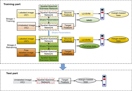
2.1. A Two-Stage Deep Domain Adaptation Framework

The framework of the TDDA method is shown in Figure 1. Figure 1 consists of training and testing parts. In the training part, we divide the training process of TDDA into two stages to train the spatial spectral network. In the testing part, a large number of unlabeled images in the target domain are classified based on the spatial spectral network. The two training stages are detailed below.

In the first stage, the inputs are the labeled samples of the source domain and unlabeled samples of the target domain. The classification Loss (margin-based loss) and domain alignment Loss (MMD) are minimized. The sample features of the source and target domains are extracted by Spatial–Spectral Siamese Network (weight sharing) [28]. Then, the distribution shift between the source domain and the target domain is minimized based on MMD. For the classification function, we use linear support vector machines instead of the softmax layer and learn to minimize margin-based loss rather than cross-entropy loss. After the training task of the first stage is completed, the weights learned are used as the initial weights of the second stage.

In the second stage, the inputs are the labeled samples of the source domain and few labeled samples of the target domain. The classification loss (margin-based loss) and domain discriminative loss (Pairwise loss) are minimized. Based on the pairwise loss, the distance between samples from different domains but the same class is minimized and the distance between samples from different classes in different domains is maximized. For the test part, the inputs are the unlabeled samples of the target domain, and the outputs are the predicted labels.

2.2. The Spatial–Spectral Network

The CNN architecture generally consists of a convolutional layer, pooling layer, and fully connected layer, and each layer is connected to its previous layer, so that abstract features of higher layers can be extracted from lower layers. Generally, deeper networks can extract more discriminative information [29], which is helpful for image classification. Neural networks usually have several fully connected layers that can learn the abstract features and output the network’s final predictions. We assume the given training data is $\left(X,Y\right)={\left\{\left(x_i,y_i\right)\right\}}_{i=1}^N$, so the feature output of the kth layer is:

$${\phi }^k\left(x_i\right)=g\left(W^k·{\phi }^{\left(k-1\right)}\left(x_i\right)+B^k\right),$$

(1)

where $W^k$ represents the weight matrix, ${\phi }^{\left(k-1\right)}$ is the feature output in the $\left(k-1\right)$th layer, $B^k$ is the bias of the kth layer, and $g(\cdot )$ is a non-linear activation function, for example, a linear unit function of rectification is $\mathrm{g}\left(x\right)=max\left(0,x\right)$ [30].

Hyperspectral images have abundant spatial and spectral information. Extracting advanced features from spatial and spectral branches respectively and fusing them can improve classification accuracy [31,32]. Therefore, in this section, the joint spatial–spectral features are extracted through the Spatial–Spectral Network.

As shown in Figure 2, the Spatial–Spectral Network has two CNN branches, which are used to extract spatial and spectral features, respectively. In the spatial branch, we first reduce the dimensionality of the input hyperspectral image with Principal Component Analysis (PCA) [33,34], and then take a pixel and its neighborhood (the neighborhood size is r = 4) as input (9 × 9 × 10); the spatial output of this branch is ${\phi }_{spa}^k\left(x_i\right)$. In the spectral branch, we take the spectral of this pixel and its neighborhood (r = 1) as input (3 × 3 × chn); the spectral output of this branch is ${\phi }_{spe}^k\left(x_i\right)$. We simultaneously feed the output of the two branches to the fully connected layer, and the joint spatial–spectral feature output is:

$${\phi }^{\left(k+1\right)}\left(x_i\right)=g\left(W^{\left(k+1\right)}·\left[{\phi }_{spa}^k\left(x_i\right)\oplus {\phi }_{spe}^k\left(x_i\right)\right]+B^{\left(k+1\right)}\right)$$

(2)

where $\oplus$ indicates that the spatial output and spectral output are connected in series, and the output ($\phi \left(x_i\right)$) can be regarded as the final joint spatial–spectral feature output.

2.3. The First Stage of TDDA

In [27], Tang demonstrated a small but consistent advantage of replacing the softmax layer with a linear support vector machine. Inspired by [27], we replaced softmax layer with SVM in our paper. SVM is generally used for binary classification. We assume that the label of a given training data is $p_i\in \left\{-1,1\right\}$. Owing to the fact that L1-SVM is not differentiable, its variant L2-SVM is adopted to minimize the square hinge loss:

$$\underset{w}{\min }\frac{1}{2}{w}^{T}w+C{\sum }_{i=1}^{N}max{\left(0,1-p_{i}f\left(\phi \left(x_i\right)\right)\right)}^2,$$

(3)

where $w$ is the normal vector of the hyperplane in space, C is the penalty coefficient, and $f(\cdot )$ is the prediction of the training data. In order to solve the classification problem of multiple classes, we adopt the one-versus-rest approach. This method constructs L SVMs to solve the classification problem where the number of classes is L. Each SVM only needs to distinguish the data of this class from the data of other classes.

In measuring the differences between domains, we consider that the source and target domains have similar distributions. Therefore, in the first stage, we use MMD to measure the distance between two different but related distributions, which can be defined as:

$${ℒ}_{MMD}=\Vert \frac{1}{N}{\sum }_{i=1}^N\phi \left(x_i^s\right)-\frac{1}{M}{\sum }_{j=1}^M\phi \left(x_j^t\right){\Vert }_2^2,$$

(4)

A common embedding can be obtained by minimizing the distribution distance with MMD, and the main statistical properties of the data in the two domains are preserved.

Therefore, the weighted training standards in the first stage can be denoted as:

$${ℒ}_{st1}=\left(1-\alpha \right){ℒ}_{lsvm}+\alpha {ℒ}_{MMD},$$

(5)

Finally, to balance the classification versus the domain alignment portion (MMD) of the loss, the classification portion is normalized and weighted by 1 − α and MMD portion by α.

2.4. The Second Stage of TDDA

In the second stage, we obtained the label information of a few target domain samples. In this stage, the network parameters in the first stage are used as initialization parameters to retrain the network. In this stage, we use pairwise loss to minimize the distribution distance between samples from different domains but with the same class and maximize the distribution distance between samples from different classes between different domains to reduce the distribution shift and learn a more discriminative deep embedding space. In this stage, the Euclidean distance between samples in different domains is:

$$d=\Vert \phi \left(x_i^s\right)-\phi \left(x_j^t\right){\Vert }_2,$$

(6)

where $\Vert \cdot {\Vert }_2$ represents the Euclidean norm.

Therefore, the Pairwise loss of samples between domains is:

$${ℒ}_{PW}=\left(1-\ell \right)\frac{1}{2}{d}^2+\ell \frac{1}{2}max{\left(0,\gamma -d\right)}^2,$$

(7)

when $\ell =0$ means that the sample classes of the source domain and the target domain are the same ($y_i^s=y_j^t$), and when $\ell =1$ means that the sample classes of the source domain and the target domain are different ($y_i^s\ne y_j^t$). $\gamma$ represents the threshold.

Therefore, the weighted training standards for the second stage can be expressed as:

$${ℒ}_{st2}=\left(1-\alpha \right){ℒ}_{lsvm}+\alpha {ℒ}_{PW},$$

(8)

Finally, to balance the classification versus the domain discriminative portion (Pairwise) of the loss, the classification portion is normalized and weighted by 1 − α and Pairwise portion by α.

3. Experiments

3.1. Data Sets Description

In this experiment, we conducted experiments on two sets of real-world hyperspectral remote sensing images, including Pavia University–Pavia Center dataset and the Shanghai–Hangzhou dataset.

First, Pavia University and Pavia Center datasets were obtained by ROSIS sensors during the air battle in Pavia in northern Italy [16]. The number of spectral bands obtained by the sensor on the datasets of the Pavia University and Pavia Center is 103 and 102, respectively. By reducing one band of the Pavia University Dataset, the spectral bands of both datasets are 102. Pavia University is a 610 × 610 pixels image, while Pavia Centre is a 1096 × 1096 pixels image, but some samples in both images do not contain any information, so they must be discarded before analysis. Therefore, the image of Pavia University is 610 × 315 pixels, and the image of Pavia Center is 1096 × 715 pixels, as shown in Figure 3a and Figure 4a, respectively. We select seven classes that they both have, including trees, asphalt, self-blocking bricks, bitumen, shadows, meadows, and bare soil, as shown in Figure 3b and Figure 4b, respectively. The names of land cover classes and number of samples for Pavia University–Pavia Center Dataset pair are listed in

Table 2. Land cover classes and the number of samples for Pavia University–Pavia Center.

Class		Number of Samples
No.	Name	Pavia University	Pavia Center
1	Trees	3064	7598
2	Asphalt	6631	3090
3	Bricks	3682	2685
4	Bitumen	1330	6584
5	Shadows	947	7287
6	Meadows	18,649	42,816
7	Bare Soil	5029	2863
	Total	39,332	72,923

.

Second, Shanghai and Hangzhou datasets were both captured by EO-1 Hyperion hyperspectral sensor in in Shanghai and Hangzhou [14]. The sensor obtained a number of spectral bands of 220 in both scenes, leaving 198 spectral bands after removing bad bands. Shanghai is 1600 × 230 pixels, and Hangzhou is 590 × 230 pixels, as shown in Figure 5a. In this experiment, we selected three classes, including water, ground/buildings and plants, as shown in Figure 5b. The names of land cover classes and number of samples for the Shanghai–Hangzhou Dataset are listed in

Table 3. Land cover classes and the number of samples for Shanghai–Hangzhou.

Class		Number of Samples
No.	Name	Shanghai	Hangzhou
1	Water	123,123	18,043
2	Ground/Building	161,689	77,450
3	Plants	83,188	40,207
	Total	368,000	135,700

.

3.2. Experimental Settings

For the source domain, 200 labeled samples per class for the source domain and 5 labeled samples per class for the target domain are randomly selected for training for each split. The remaining labeled samples in the target domain are used as test samples to evaluate the classification performance.

In the Spatial–Spectral Network, each branch of the model consists of two convolutional layers, one pooling layer and one dropout layer. The spatial and spectral features obtained from the two branches are combined to obtain a joint spatial–spectral feature, and the final joint spatial–spectral feature is obtained through three fully connected layers. We get the parameters of all network layers except the last layer, and transfer them to the second stage to retrain the network.

In the TDDA method, the first and second training stages are optimized using Adam optimization algorithm [35]. In the first stage, the training epoch is set to 100, the batch size is set to 128, and the learning rate is set to 0.001. In the second stage, the training epoch is set to 80, the batch size is set to 80, and the learning rates of the Pavia University–Pavia Center Datasets and the Shanghai–Hangzhou Datasets are set to 0.0001 and 0.00001, respectively. The specific parameters of the network are shown in

Table 4. Network parameters of TDDA.

	Spectral Branch	Spatial Branch
Number of conv. layers	2	2
Number of filters	16,32	32,128
Filters size of conv. layer	1 × 1 × 16	3 × 3
Number of pooling layers	1	1
Filters size of pooling layer	1 × 1 × 5	3 × 3
Dropout	0.25
Fully Connected layer1	1000
Fully Connected layer2	100
Output	L

. In addition, we performed a comparative experiment on the choice of the equilibrium parameter α on the Pavia University → Pavia Center dataset. As shown in

Table 5. Equilibrium parameter α of TDDA method.

α	Overall Accuracy (OA)	Average Accuracy (AA)
0.25	94.19 ± 0.64	93.96 ± 0.27
0. 5	90.53 ± 0.67	92.35 ± 0.26
0.75	92.64 ± 0.70	93.03 ± 0.29

, when the value of the equilibrium parameter α is 0.25, both the OA and AA of the experiment achieve the best value, and the result has the smallest degree of dispersion. Therefore, we take α = 0.25 as the equilibrium parameter of the experiment.

In order to verify the effectiveness of our method, we compared the TDDA method with some of the latest methods such as Mei et al. [16], Yang et al. [17], Wang et al. + fine-tuning (FT) [25]. In addition, the first stage + fine-tuning (First-Stage + FT) is also compared. In order to ensure the fairness of the experiment, we select one to five labeled target domain samples per class in all experiments. For Mei et al, Yang et al, Wang et al. +FT and First-Stage +FT methods, the labeled target domain samples are mainly used to fine-tune the network model. For TDDA, the labeled target domain samples are used to train the network model based on pairwise loss and margin-based loss.

For the classification results of different datasets, we consider the following four cases: Pavia University → Pavia Center, Pavia Center → Pavia University, Shanghai → Hangzhou and Hangzhou → Shanghai, which respectively represent the source dataset → the target dataset. All of the above experiments were performed on a workstation equipped with an AMD Ryzen 5 4000 Quad-Core Processor 3.2 GHZ and 8 GB RAM.

For a fair comparison, the same training and test data sets are utilized in all methods. The overall accuracy (OA), average accuracy (AA), and kappa coefficients are used to evaluate the classification performance of all methods. All methods are performed 10 times, and the average result which adds the standard deviation obtained from 10 runs, was used to reduce the impact of random selection.

3.3. Experimental Results

To prove the superiority of the proposed TDDA method, we compared our method with other methods on two sets of datasets. In these experiments, the training set consists of two parts, one part randomly selects 200 labeled samples from the source domain, and the other part randomly selects 5 labeled samples from the target domain. The remaining samples in the target domain are used as the test set. In

Table 6. Classification accuracy and kappa (%) on Pavia University → Pavia Center dataset.

Class	Mei et al.	Yang et al.	Wang et al. +FT	First-Stage + FT	TDDA
Trees	71.49	80.41	88.20	84.46	92.81
Asphalt	95.23	70.26	94.34	84.21	93.56
Bricks	89.22	55.25	69.99	91.56	98.56
Bitumen	68.30	78.81	80.52	73.51	88.27
Shadows	88.88	77.88	88.28	89.49	89.18
Meadows	97.36	73.90	97.99	98.08	95.59
Bare soil	99.97	73.90	99.58	99.70	99.90
OA	90.91 ±0.97	75.51 ±1.56	93.10 ±0.61	92.83 ±0.79	94.19 ±0.64
AA	87.20 ±0.90	76.28 ±1.00	88.42 ±0. 86	88.11 ±0.78	93.96 ±0.27
Kappa	85.59 ±1.47	64.63 ±1.82	89.21 ±1.16	88.19 ±0.97	90.89 ±0.95

,

Table 7. Classification accuracy and kappa (%) on Pavia Center → Pavia University dataset.

Class	Mei et al.	Yang et al.	Wang et al. +FT	First-Stage + FT	TDDA
Trees	94.40	94.72	97.47	94.45	98.33
Asphalt	74.06	87.77	63.58	57.93	84.49
Bricks	88.74	73.39	96.92	81.65	95.07
Bitumen	77.24	23.05	96.75	95.14	94.87
Shadows	99.68	99.47	99.42	98.63	99.98
Meadows	63.33	59.91	81.33	73.51	86.74
Bare soil	50.16	22.65	39.10	73.53	27.27
OA	69.54 ±1.50	63.59 ±1.37	76.61 ±1.39	75.22 ±1.41	81.03 ±0.77
AA	78.24 ±1.98	65.85 ±0.86	82.08 ±0.89	82.13 ±1.16	83.82 ±0.78
Kappa	60.12 ±1.83	52.60 ±1.42	67.74 ±1.82	67.17 ±1.71	73.26 ±1.05

,

Table 8. Classification accuracy and kappa (%) on Shanghai → Hangzhou dataset.

Class	Mei et al.	Yang et al.	Wang et al. +FT	First-Stage + FT	TDDA
Water	89.80	99.40	93.56	92.56	99.59
Ground/Building	92.68	87.10	83.80	83.87	95.13
Plant	95.86	54.92	96.33	85.07	95.04
OA	93.24 ±0.91	79.20 ±1.26	88.81 ±1.55	85.66 ±1.04	95.65 ±0.24
AA	92.78 ±0.59	80.48 ±0.92	91.23 ±0.60	87.86 ±1.36	96.52 ±0.27
Kappa	88.17 ±1.52	62.98 ±2.04	81.02 ±2.38	75.34 ±1.17	92.42 ±0.41

and

Table 9. Classification accuracy and kappa (%) on Hangzhou → Shanghai dataset.

Class	Mei et al.	Yang et al.	Wang et al. +FT	First-Stage + FT	TDDA
Water	98.08	92.99	98.76	95.30	95.27
Ground/Building	98.65	87.17	84.43	88.29	93.76
Plant	80.90	99.98	99.56	94.36	99.78
OA	94.45 ±0.42	92.02 ±0.35	92.64 ±0.89	92.23 ±1.17	95.62 ±0.25
AA	92.54 ±0.32	93.38 ±0.27	94.25 ±0.63	93.00 ±0.48	96.27 ±0.20
Kappa	91.46 ±0.56	87.79 ±0.52	88.79 ±1.32	88.09 ±1.69	93.25 ±0.38

, overall accuracy (OA), average accuracy (AA), and kappa coefficient are utilized as performance criteria. Table 6, Table 7, Table 8 and Table 9 list the experimental results of different methods on Pavia University → Pavia Center, Pavia Center → Pavia University, Shanghai → Hangzhou and Hangzhou → Shanghai datasets. Figure 6, Figure 7, Figure 8 and Figure 9 show the corresponding classification maps of all methods. As can be seen from the bold classification accuracy in Table 5, Table 6, Table 7 and Table 8, TDDA performs better in OA and AA than other methods in all cases and has a smaller standard deviation in most cases, which proves the effectiveness and stability of the TDDA method. In addition, as can be seen from the classification maps in Figure 6, Figure 7, Figure 8 and Figure 9, compared with other methods, the classification map obtained by TDDA method proposed in this paper is the most accurate. The detailed analysis of Table 6, Table 7, Table 8 and Table 9 is as follows.

Table 6 shows the classification performance from Pavia University to Pavia Center dataset. It can be seen from Table 6 that compared with the fine-tuning strategy (Mei et al. and Yang et al.), the domain shift reduction + fine-tuning strategy (Wang et al. +FT and First-Stage +FT) achieves better classification performance. Compared with Mei et al. and Yang et al. methods, Wang et al. +FT increases OA by 2.19% and 17.5% respectively, and First-Stage +FT increases OA by 1.92% and 17.32% respectively. These results show that domain shift reduction + fine-tuning strategy can better handle data shift problem. It is worth noting that compared with the Yang et al. method, the Mei et al. method increases OA by 15.4%. The main reason is that Mei et al.’ method fine-tuned the weights of the low, mid and top-layers of the network, which can extract discriminative features for the target domain. Since First-Stage +FT only adopts MMD metric criteria, the classification performance is slightly lower than the method of Wang et al. +FT. Compared with the First-Stage +FT method, TDDA increases OA by 1.36%, which shows that the second stage plays an important role. Compared with the second-ranked method (Wang et al. + FT), our proposed TDDA increases OA by 1.09%, which shows that TDDA not only reduces the domain shift, but also obtains a more discriminative feature space.

Table 7 shows the classification performance from Pavia Center to Pavia University dataset. As can be seen from Table 7, the method with the domain shift reduction + fine-tuning strategy is better than the method with the fine-tuning strategy. Compared with Mei et al. and Yang et al. methods, Wang et al. +FT increases OA by 7.07% and 13.02% respectively, and First-Stage +FT increases OA by 5.68% and 12.63% respectively. The proposed TDDA achieves the best classification performance. Compared with the fine-tuning strategy (Mei et al. and Yang et al.), TDDA increases OA by 11.49% and 17.44% respectively. Compared with the domain shift reduction + fine-tuning strategy (Wang et al. +FT and First-Stage +FT), TDDA increases OA by 4.42% and 5.81% respectively. It is worth noting that TDDA increases OA by 5.81% more than First-Stage +FT, which fully demonstrates the role of the second stage of TDDA. Compared with the second-ranked method (Wang et al. + FT), TDDA increases OA by 4.42%.

Table 8 shows the classification performance from the Shanghai to Hangzhou dataset. It can be seen from Table 8 that compared with the fine-tuning strategy (Yang et al.), the domain shift reduction + fine-tuning strategy (Wang et al. +FT and First-Stage +FT) achieve better classification performance. It is worth noting that the Mei et al. method with fine-tuning strategy is superior to the Wang et al. +FT and First-Stage +FT. The reason is that two fine-tunings were used in the method of Mei et al. The first fine-tuning can extract discriminative features for the target domain. In the second fine-tuning, only top layers are trained using the discriminative features from the target domain, which can better perform knowledge transfer. However, our proposed TDDA still achieves the best classification performance. Compared with the second-ranked method (Mei et al.), TDDA increases OA by 2.41%, which demonstrates the stability and superiority of TDDA.

Table 9 shows the classification performance from the Hangzhou to Shanghai dataset. As can be seen from Table 9, Wang et al. +FT and First-Stage +FT methods increase OA by 0.62% and 0.21%. Compared with Yang et al, Wang et al. +FT and First-Stage +FT methods, Mei et al. method increases OA by 2.43%, 1.81% and 2.22%. However, the proposed TDDA is still the best to obtain classification performance. Compared with the domain shift reduction + fine-tuning strategy (Wang et al. +FT and First-Stage +FT), TDDA increases OA by 2.98% and 3.39% respectively. Compared with the fine-tuning strategy (Mei et al. and Yang et al.), TDDA increases OA by 1.17% and 3.6% respectively, which further demonstrates the stability and superiority of TDDA.

The training and testing times provide a direct measure of computational efficiency for TDDA. All experiments were carried out on a workstation equipped with an AMD Ryzen 5 4000 Quad-Core Processor 3.2 GHZ and 8 GB RAM.

Table 10. Training and test time for each method in four cases.

		Mei et al.	Yang et al.	Wang et al. + FT	First-Stage + FT	TDDA
Pavia university → Pavia center	Train (s)	83.82	91.42	108.10	76.08	883.69
	Test (s)	1.47	3.61	13.91	11.76	15.04
Pavia center → Pavia university	Train (s)	74.30	75.98	102.97	71.39	889.25
	Test (s)	0.85	1.80	6.02	5.54	7.32
Shanghai → Hangzhou	Train (s)	37.26	39.00	78.92	48.05	526.90
	Test (s)	2.55	5.98	33.06	21.36	42.97
Hangzhou → Shanghai	Train (s)	38.64	43.88	106.65	54.65	516.87
	Test (s)	3.69	15.77	69.66	44.52	127.64

shows the training and testing time of different methods in different situations. It can be seen that the training of the TDDA method takes the longest time. This is because the training of TDDA is divided into two stages, and especially in the second stage, samples with the same label between domains and samples with different labels between domains are fed into the network in pairs, which increases the computational time. Although TDDA is longer than the training time of other methods, the classification accuracies of TDDA are better than all other methods.

In addition, in order to better verify the effectiveness of the proposed method, we extend the above experiment, where one to five labeled samples are randomly selected from the target domain. In these experiments, the training set consists of 200 labeled samples from the source domain and one to five labeled samples from the target domain. The remaining samples in the target domain are used as the test set. The classification results are shown in Figure 10, Figure 11, Figure 12 and Figure 13. The training samples of each class in the source domain are maintained at 200, while the number of training samples of each class in the target domain varies from 1 to 5.

Figure 10 shows the classification performance of each method on Pavia University → Pavia Center. It can be seen from Figure 10 that the classification performance of the TDDA method is better than other methods regardless of the number of labeled samples in the target domain, which indicates that when the number of labeled samples in the target domain is small, TDDA can also learn more discriminative features to achieve better classification performance of hyperspectral images. Figure 11 shows the classification performance of all methods on Pavia Center → Pavia University dataset. As can be seen from Figure 11, TDDA has obvious advantages over other methods.

Figure 12 and Figure 13 show the classification performance of all methods on Shanghai → Hangzhou and Hangzhou → Shanghai datasets. As can be seen from Figure 12 and Figure 13, with the increase of the number of labeled target samples per category, the OAs and AAs of TDDA do not change significantly. However, overall there is still a slight upward trend. This result is due to the pairwise loss and margin-based loss in the second stage, which can extract more discriminative features. In addition, the classification performance of the model is better when there is only one labeled sample per class in the target domain, possibly because of the small number of categories in the Shanghai–Hangzhou dataset (only three categories).

As can be seen from Figure 10, Figure 11, Figure 12 and Figure 13, the methods using the fine-tuning strategy are not stable compared with the methods using the domain shift reduction + fine-tuning strategy in different experiments. From the results of Figure 10, Figure 11, Figure 12 and Figure 13, it can be concluded that when the source domain has sufficient labeled samples and the target domain has only a small number of labeled samples, compared with other methods, TDDA is the most effective and stable classification method.

4. Discussion

Firstly, Mei et al. and Yang et al. methods directly use fine-tuning strategy to perform knowledge transfer, and the labeled samples in target domain are mainly used to fine-tune the corresponding network model. However, Mei et al. method is different from Yang et al. method. Mei et al. method is actually fine-tuned twice. The first fine-tuning extracts discriminative features for the target domain, where the low, mid and top-layers of the network are retrained using training samples from the target domain. In the second fine-tuning, only top layers are trained using the discriminative features of training samples from the target domain. However, in Yang et al. method, low and mid-layers of the network are pretrained and transferred from other data sources; only the weights of top layers are fine-tuned with limited training samples extracted from the target domain. As can be seen from Table 5, Table 6, Table 7 and Table 8 and Figure 10, Figure 11, Figure 12 and Figure 13, Mei et al. method is superior to Yang et al. method in most cases, which shows that only fine-tuning the weight of the top layer is not as good as fine-tuning the weight of the lower, middle, and top layers.

Secondly, Wang et al. +FT and First-Stage +FT methods use domain shift reduction strategy to minimize the distribution distance between domains, and then the fine-tuning strategy is used to perform knowledge transfer. As can be seen from Table 5, Table 6, Table 7 and Table 8 and Figure 10, Figure 11, Figure 12 and Figure 13, the methods using the domain shift reduction + fine-tuning strategy are more stable compared with the methods only using the fine-tuning strategy in different experiments, which indicates that a more suitable common feature space for the source and target domain can be obtained by minimizing the distribution distance between domains, and more stable classification results can be achieved by fine-tuning on the common feature space.

Thirdly, TDDA uses domain shift reduction strategy to minimize the distribution distance between two domains at different stages, where labeled samples from the target domain are used to learn more discriminative feature spaces rather than fine-tuning the corresponding network model. The above experimental results show that in the case of very few labeled samples for the target domain, for the method based on deep learning, the proposed TDDA method has a very obvious advantage in classification accuracy compared to other methods. As can be seen from Table 5, Table 6, Table 7 and Table 8, compared with the First-Stage +FT method, TTDA increases OA by 1.36%, 6.08%, 9.99%, and 3.39% respectively, which fully demonstrates the effectiveness of the second stage. Compared with Wang et al. +FT method, TTDA increases OA by 1.09%, 4.42%, 6.84%, and 2.98% respectively. It can be seen from these experiments that TTDA not only reduces the domain shift between the source and target domains, but also learns a discriminative embedded feature space that is more suitable for the target domain. As can be seen from Table 5, Table 6, Table 7 and Table 8, compared with only the fine-tuning strategy (Mei et al. and Yang et al. methods), TTDA also achieve better classification performance. The OA of TTDA is 3.28%, 11.49%, 1.17%, and 1.17% higher than Mei et al. method respectively. The OA of TTDA is 18.68%, 17.44%, 16.45%, and 3.6% higher than Yang et al. method respectively. In addition, it can be seen from Figure 10, Figure 11, Figure 12 and Figure 13 that even with fewer labeled samples from the target domain, TDDA still has better classification performance than other methods, which demonstrates the effectiveness and stability of TTDA.

Finally, the proposed TDDA method is divided into two training stages, which leads to its relatively long training time and means that TDDA is more computationally expensive than other methods. Fortunately, the adoption of GPU has greatly alleviated the extra computational costs.

5. Conclusions

In this paper, we propose a novel two-stage deep domain adaptation method for hyperspectral images classification. Compared with the previous networks, TDDA consists of two training stages and designs a Spatial–Spectral Siamese network for extracting spatial–spectral feature. The first stage is to obtain a deep common embedding feature space by minimizing MMD and margin-based loss, which can reduce the domain shift between the source and target domains. In the second stage, based on pair loss and margin-based loss, the few labeled samples from the target domain are used to learn a deep common embedding feature space that is more discriminative to the target domain. Compared with other methods, this method can simultaneously extract the abundant joint spatial–spectral information in the source domain and the target domain through the Spatial–Spectral Siamese network; minimize three criteria (including MMD, pairwise loss, and margin-based loss) to reduce the distribution shift between the two domains; and use a few labeled target domain samples to learn a more discriminative deep common embedding space, thereby improving the classification performance of the target domain. Analysis of experimental results on two sets of hyperspectral remote sensing images demonstrates that our method not only performs better than the other methods, but also extracts more discriminative feature representations to the target domain. In the future, we will further research the classification of hyperspectral images based on heterogeneous transfer learning.

References

1. Liang, L.; Di, L.; Zhang, L.; Deng, M.; Qin, Z.; Zhao, S.; Lin, H. Estimation of crop LAI using hyperspectral vegetation indices and a hybrid inversion method. Remote Sens. Environ. 2015, 165, 123–134. [Google Scholar] [CrossRef]
2. Laurin, G.V.; Chan, J.C.W.; Chen, Q.; Lindsell, J.A.; Coomes, D.A.; Guerriero, L.; Del Frate, F.; Miglietta, F.; Valentini, R. Biodiversity mapping in a tropical West African forest with airborne hyperspectral data. PLoS ONE 2014, 9, e97910. [Google Scholar]
3. Yokoya, N.; Chan, J.C.W.; Segl, K. Potential of Resolution-Enhanced Hyperspectral Data for Mineral Mapping Using Simulated EnMAP and Sentinel-2 Images. Remote Sens. 2016, 8, 172. [Google Scholar] [CrossRef] [Green Version]
4. Lu, X.; Li, X.; Mou, L. Semi-Supervised Multitask Learning for Scene Recognition. IEEE Trans. Cybern. 2015, 45, 1967–1976. [Google Scholar] [PubMed]
5. Yuen, P.W.T.; Richardson, M. An introduction to hyperspectral imaging and its application for security, surveillance and target acquisition. Imaging Sci. J. 2010, 58, 241–253. [Google Scholar] [CrossRef]
6. Li, W.; Wu, G.; Zhang, F.; Du, Q. Hyperspectral image classification using deep pixel-pair features. IEEE Trans. Geosci. Remote Sens. 2017, 55, 844–853. [Google Scholar] [CrossRef]
7. Chen, Y.; Jiang, H.; Li, C.; Jia, X.; Ghamisi, P. Deep feature extraction and classification of hyperspectral images based on convolutional neural networks. IEEE Trans. Geosci. Remote Sens. 2016, 54, 6232–6251. [Google Scholar] [CrossRef] [Green Version]
8. Li, Z.; Huang, L.; He, J. A Multiscale Deep Middle-level Feature Fusion Network for Hyperspectral Classification. Remote Sens. 2019, 11, 695. [Google Scholar] [CrossRef] [Green Version]
9. Li, Y.; Zhang, H.; Shen, Q. Spectral–spatial classification of hyperspectral imagery with 3D convolutional neural network. Remote Sens. 2017, 9, 67. [Google Scholar] [CrossRef] [Green Version]
10. Zhong, Z.; Li, J.; Luo, Z.; Chapman, M. Spectral-Spatial Residual Network for Hyperspectral Image Classification: A 3-D Deep Learning Framework. IEEE Trans. Geosci. Remote Sens. 2017, 56, 847–858. [Google Scholar] [CrossRef]
11. Zhao, W.; Du, S. Learning multiscale and deep representations for classifying remotely sensed imagery. ISPRS J. Photogramm. Remote Sens. 2016, 113, 155–165. [Google Scholar] [CrossRef]
12. Camps-Valls, G.; Marsheva, T.V.B.; Zhou, D. Semi-supervised graph-based hyperspectral image classification. IEEE Trans. Geosci. Remote Sens. 2007, 45, 3044–3054. [Google Scholar] [CrossRef]
13. Zhou, X.; Prasad, S. Active and semisupervised learning with morphological component analysis for hyperspectral image classification. IEEE Geosci. Remote Sens. Lett. 2017, 14, 1348–1352. [Google Scholar] [CrossRef]
14. Ye, M.C.; Qian, Y.T.; Zhou, J.; Tang, Y.Y. Dictionary learning-based feature-level domain adaptation for cross-scene hyperspectral image classification. IEEE Trans. Geosci. Remote Sens. 2017, 55, 1544–1562. [Google Scholar] [CrossRef] [Green Version]
15. Jiao, L.; Liang, M.; Chen, H.; Yang, S.; Liu, H.; Cao, X. Deep Fully Convolutional Network-Based Spatial Distribution Prediction for Hyperspectral Image Classification. IEEE Trans. Geosci. Remote Sens. 2017, 55, 5585–5599. [Google Scholar] [CrossRef]
16. Mei, S.; Ji, J.; Hou, J.; Li, X.; Du, Q. Learning Sensor-Specific Spatial-Spectral Features of Hyperspectral Images via Convolutional Neural Networks. IEEE Trans. Geosci. Remote Sens. 2017, 55, 4520–4533. [Google Scholar] [CrossRef]
17. Yang, J.; Zhao, Y.Q.; Chan, J.C.W. Learning and Transferring Deep Joint Spectral–Spatial Features for Hyperspectral Classification. IEEE Trans. Geosci. Remote Sens. 2017, 55, 4729–4742. [Google Scholar] [CrossRef]
18. Tuia, D.; Persello, C.; Bruzzone, L. Domain adaptation for the classification of remote sensing data: An overview of recent advances. IEEE Geosci. Remote Sens. Mag. 2016, 4, 41–57. [Google Scholar] [CrossRef]
19. Long, M.; Zhu, H.; Wang, J.; Jordan, M.I. Deep Transfer Learning with Joint Adaptation Networks. In Proceedings of the 2017 International Conference on Machine Learning (ICML), Sydney, NSW, Australia, 6–11 August 2017; pp. 2208–2217. [Google Scholar]
20. Yan, H.; Ding, Y.; Li, P.; Wang, Q.; Xu, Y.; Zuo, W. Mind the Class Weight Bias: Weighted Maximum Mean Discrepancy for Unsupervised Domain Adaptation. In Proceedings of the 2017 IEEE Conference on Computer Vision and Pattern Recognition (CVPR), Honolulu, HI, USA, 21–26 July 2017; IEEE: Piscataway, NJ, USA, 2017; pp. 945–954. [Google Scholar]
21. Sun, Z.; Wang, C.; Wang, H.; Li, J. Learn multiple-kernel SVMs for domain adaptation in hyperspectral data. IEEE Geosci. Remote Sens. Lett. 2013, 10, 1224–1228. [Google Scholar]
22. Deng, C.; Liu, X.; Li, C.; Tao, D. Active multi-kernel domain adaptation for hyperspectral image classification. Pattern Recognit. 2018, 77, 306–315. [Google Scholar] [CrossRef] [Green Version]
23. Yang, H.; Crawford, M. Domain adaptation with preservation of manifold geometry for hyperspectral image classification. IEEE J. Sel. Top. Appl. Earth Obs. Remote Sens. 2015, 9, 543–555. [Google Scholar] [CrossRef]
24. Othman, E.; Bazi, Y.; Melgani, F.; Alhichri, H.; Alajlan, N.; Zuair, M. Domain adaptation network for cross-scene classification. IEEE Trans. Geosci. Remote Sens. 2017, 55, 4441–4456. [Google Scholar] [CrossRef]
25. Wang, Z.; Du, B.; Shi, Q.; Tu, W. Domain Adaptation with Discriminative Distribution and Manifold Embedding for Hyperspectral Image Classification. IEEE Geosci. Remote Sens. Lett. 2019, 16, 1155–1159. [Google Scholar] [CrossRef]
26. Motiian, S.; Piccirilli, M.; Adjeroh, D.A.; Doretto, G. Unified Deep Supervised Domain Adaptation and Generalization. In Proceedings of the 2017 IEEE International Conference on Computer Vision (ICCV), Venice, Italy, 22–29 October 2017; IEEE: Piscataway, NJ, USA, 2017; pp. 5716–5726. [Google Scholar]
27. Yichuan, T. Deep learning using linear support vector machines. arXiv 2015, arXiv:1306.0239, 2015. [Google Scholar]
28. Chopra, S.; Hadsell, R.; LeCun, Y. Learning a Similarity Metric Discriminatively, with Application to Face Verification. In Proceedings of the 2005 IEEE International Conference on Computer Vision and Pattern Recognition (CVPR), San Diego, CA, USA, 20–26 June 2005; IEEE: Piscataway, NJ, USA, 2005; pp. 539–546. [Google Scholar]
29. Simonyan, K.; Zisserman, A. Very Deep Convolutional Networks for Large-Scale Image Recognition. In Proceedings of the 2015 International Conference on Learning Representations (ICLR), San Diego, CA, USA, 7–9 May 2015; pp. 1–14. [Google Scholar]
30. Krizhevsky, A.; Sutskever, I.; Hinton, G.E. ImageNet classification with deep convolutional neural networks. Commun. ACM 2017, 60, 84–90. [Google Scholar] [CrossRef]
31. Liao, W.; Mura, M.D.; Chanussot, J.; Pižurica, A. Fusion of spectral and spatial information for classification of hyperspectral remote-sensed imagery by local graph. IEEE J. Sel. Topics Appl. Earth Obs. Remote Sens. 2016, 9, 583–594. [Google Scholar] [CrossRef]
32. Li, Z.; Huang, L.; Zhang, D.; Liu, C.; Wang, Y.; Shi, X. A deep network based on multiscale spectral-spatial fusion for Hyperspectral Classification. In Proceedings of the 2018 International Conference on Knowledge Science, Engineering and Management (KSEM), Jilin, China, 17–19 August 2018; pp. 283–290. [Google Scholar]
33. Guo, X.; Huang, X.; Zhang, L.; Zhang, L.; Plaza, A.; Benediktsson, J.A. Support tensor machines for classification of hyperspectral remote sensing imagery. IEEE Trans. Geosci. Remote Sens. 2016, 54, 3248–3264. [Google Scholar] [CrossRef]
34. Makantasis, K.; Karantzalos, K.; Doulamis, A.D.; Doulamis, N.D. Deep Supervised Learning for Hyperspectral Data Classification Through Convolutional Neural Networks. In Proceedings of the 2015 IEEE International Geoscience and Remote Sensing Symposium (IGARSS), Milan, Italy, 26–31 July 2015; pp. 4959–4962. [Google Scholar]
35. Kingma, D.P.; Ba, J.A. A Method for Stochastic Optimization. arXiv 2014, arXiv:1412.6980. [Google Scholar]
Figure 1. The Framework of the two-stage deep domain adaptation (TDDA) method.
Remotesensing 12 01054 g001
Figure 2. The structure of the Spatial–Spectral Network.
Remotesensing 12 01054 g002
Figure 3. (a) False-color image of Pavia University dataset. (b) Ground truth of Pavia University dataset.
Remotesensing 12 01054 g003
Figure 4. (a) False-color image of Pavia Center dataset. (b) Ground truth of Pavia Center dataset.
Remotesensing 12 01054 g004
Figure 5. Source and target scenes in Shanghai–Hangzhou datasets. Top: Shanghai. Bottom: Hangzhou. (a) False-color image. (b) Ground truth.
Remotesensing 12 01054 g005
Figure 6. The classification maps of different methods for Pavia University → Pavia Center dataset. (a) Yang et al. method. (b) Mei et al. method. (c) Wang et al. +FT method. (d) First-Stage + FT method. (e) TDDA method. (f) Original map.
Remotesensing 12 01054 g006
Figure 7. The classification maps of different methods on Pavia Center → Pavia University dataset. (a) Yang et al. method. (b) Mei et al. method. (c) Wang et al. +FT method. (d) First-Stage + FT. (e) TDDA method. (f) Original map.
Remotesensing 12 01054 g007
Figure 8. The classification maps of different methods on Shanghai → Hangzhou dataset. (a) Yang et al. method. (b) Mei et al. method. (c) Wang et al. +FT method. (d) First-Stage + FT method. (e) TDDA method. (f) Original map.
Remotesensing 12 01054 g008
Figure 9. The classification maps of different methods on Hangzhou → Shanghai dataset. (a) Yang et al. method. (b) Mei et al. method. (c) Wang et al. +FT method. (d) First-Stage + FT method. (e) TDDA method. (f) Original map.
Remotesensing 12 01054 g009
Figure 10. The classification results of different methods with different labeled samples in target domain on Pavia University → Pavia Center dataset. (a) OA. (b) AA.
Remotesensing 12 01054 g010
Figure 11. The classification results of different methods with different labeled samples in target domain on Pavia Center → Pavia University dataset. (a) OA. (b) AA.
Remotesensing 12 01054 g011
Figure 12. The classification results of different methods with different labeled samples in target domain on Shanghai → Hangzhou dataset. (a) OA. (b) AA.
Remotesensing 12 01054 g012
Figure 13. The classification results of different methods with different labeled samples in target domain on Hangzhou → Shanghai dataset. (a) OA. (b) AA.
Remotesensing 12 01054 g013