Letter

Developing a Gap-Filling Algorithm Using DNN for the Ts-VI Triangle Model to Obtain Temporally Continuous Daily Actual Evapotranspiration in an Arid Area of China

1
Institute of RS and GIS, School of Earth and Space Sciences, Peking University, Beijing 100871, China
2
Carey Business School, Johns Hopkins University, Washington, DC 20036, USA
3
School of Civil Engineering and Environmental Science, University of Oklahoma, Norman, OK 73019, USA
*
Author to whom correspondence should be addressed.
Remote Sens. 2020, 12(7), 1121; https://doi.org/10.3390/rs12071121
Submission received: 28 February 2020 / Revised: 26 March 2020 / Accepted: 31 March 2020 / Published: 1 April 2020
(This article belongs to the Section Remote Sensing Communications)

Abstract

:
Temporally continuous daily actual evapotranspiration (ET) data play a critical role in water resource management in arid areas. As a typical remotely sensed land surface temperature (LST)-based ET model, the surface temperature-vegetation index (Ts-VI) triangle model provides direct monitoring of ET, but these estimates are temporally discontinuous due to cloud contamination. In this work, we present a gap-filling algorithm (TSVI_DNN) using a deep neural network (DNN) with the Ts-VI triangle model to obtain temporally continuous daily actual ET at regional scale. The TSVI_DNN model is evaluated against in situ measurements in an arid area of China during 2009–2011 and shows good agreement with eddy covariance (EC) observations. The temporal coverage was improved from 16.1% with the original Ts-VI tringle model to 67.1% with the TSVI_DNN model. The correlation coefficient (R), root mean square error (RMSE), bias, and mean absolute difference (MAD) are 0.9, 0.86 mm d−1, −0.16 mm d−1, and 0.65 mm d−1, respectively. When compared with the National Aeronautics and Space Administration (NASA) official MOD16 version 6 ET product, estimates of ET using TSVI_DNN are improved by approximately 49.2%. The method presented here can potentially contribute to enhanced water resource management in arid areas, especially under climate change.

Graphical Abstract

1. Introduction

Evapotranspiration (ET) is a critical component of the water cycle and water balance because it links a number of ecological and hydrological processes [1]. In arid areas, actual ET is a vital consumptive use of water derived from precipitation and irrigation, thereby affecting crop yield [2]. Hence, actual ET is a key measurement for irrigation programs, particularly where there is insufficient precipitation to meet crop growth requirements [3,4]. However, as a result of increased irrigation, drinking water demands, and urban water usage, groundwater levels have decreased significantly through over-pumping [5,6,7]. To improve both water use efficiency and the level of water resource management to balance these different water demands, it is necessary to obtain temporally continuous daily actual ET data to more accurately calculate total water consumption.
The surface temperature-vegetation index (Ts-VI) model is a typical remotely sensed land surface temperature (LST)-based ET model [8]. It depends primarily on LST and is presently most applicable for providing direct, accurate estimates of ET in arid and semi-arid areas o regional scales. Process-based models (e.g., the Penman-Monteith model [9]) have poor performance due to their lack of reliable root zone soil moisture and use of a less-than-suitable surrogate to calculate canopy conductance [10,11]. When compared with surface energy balance models (e.g., Surface Energy Balance Algorithm for Land (SEBAL) [12] and Surface Energy Balance System (SEBS) [13]), the Ts-VI triangle model shows more flexibility, relying mainly on the feature space shape constructed by the scatter plot of LST and a vegetation index (e.g., Normalized Difference Vegetation Index (NDVI)). It is then able to estimate ET directly using the resulting evaporative fraction and does not need to make the complex corrections required when replacing aerodynamic temperature by LST [13,14]. In addition, by taking advantage of the spatial variability in LST and its relationship with VI, the Ts-VI triangle model reduces its sensitivity to LST retrieval errors. Previous studies have shown that the accuracy of the Ts-VI triangle model is approximately 1 mm d−1 or less [15,16].
However, like most LST-based ET models, the Ts-VI triangle model is constrained to working only under clear-sky conditions, leaving a number of gaps in the estimates of ET and resulting in discontinuous data because of the high sensitivity of LST to clouds [11]. Various attempts have been made to reduce the effect of clouds. For instance, Zhu [17] proposed a ‘universal Ts-VI triangle method’ to obtain ET under all clear-sky conditions, resolving the issue of there being too few pixels in the feature space by combining the ‘time domain triangle method’ and the ‘space domain triangle method’. However, this method requires two steps to get from once daily remote sensing measurements to temporally continuous daily ET. These steps include scaling instantaneous observations from the Ts-VI model into daily ET and filling gaps to create continuous daily estimates. Previous studies focused mainly on the first step, and at least five methods have been developed to scale instantaneous observations from the Ts-VI model into daily ET estimates [18]. These methods include the evaporative fraction method [19], the incoming solar radiation method [20], and the reference ET fraction method [21]. These methods require stable weather conditions to reduce uncertainty. There have also been studies regarding gap-filling methods to improve LST-based ET estimation, such as the moving window averaged Bowen ratio and available water running pools [22,23,24]. Considering the number of previous studies that have focused on scaling instantaneous estimates into daily ET and the true demand for temporally continuous daily ET in water resource management, this study focuses primarily on how to obtain temporally continuous daily ET from daily ET estimates that occur only under clear-sky conditions.
The traditional machine learning method has been examined, with the goal of improving performance in filling gaps in flux tower observation-based regional ET and potential ET [24,25,26]. As a data-driven method, an artificial neural network has the potential to be used to obtain temporally continuous ET based on limited ET estimates from the Ts-VI triangle model [27]. Meanwhile, the deep neural network (DNN), characterized by having additional hidden layers, provides greater ability than a traditional shallow neural network [28] to find the complex relationship between ET and reference data. DNNs have been widely used and have shown outstanding performance in water science studies to solve traditionally difficult problems, such as predictions of soil moisture and improved quality for satellite precipitation products [29,30,31].
The main objective of this study, therefore, is to develop a gap-filling algorithm using DNN with the Ts-VI triangle model to obtain temporally continuous daily actual ET by overcoming problems with cloud contamination and testing the resulting model in an arid area of China.

2. Materials and Methods

2.1. Study Area and In Situ Measurements

The study area is an agricultural region located in the middle reaches of the Heihe River basin of China (Figure 1a) because it is a typical arid area with an annual precipitation of about 150 mm. It lies in an area that ranges from 38.5°~ 40.5°N and 98°~101°E with elevations from 1200 to 1700 m. The primary crop is spring maize, which grows well—the result of at least five irrigation events every year. There are more than ten eddy covariance (EC) stations in the area with a footprint of 200-300 m. In addition to EC data, there are in situ data collected from the Watershed Allied Telemetry Experimental Research (WATER) [20] from 2008. In this work, two in situ datasets were used (Figure 1b): (1) a three-year EC observation dataset at the Yingke station (YK), and (2) an EC network having six EC stations with measurements taken during May-September 2012. Daily ET was aggregated from 30-min observations after removing the days having gaps due to rainfall and instrument malfunctions. These datasets were provided by the National Tibetan Plateau Data Center (http://data.tpdc.ac.cn) [32,33,34].

2.2. Data

Thirteen remote sensing and meteorological forcing datasets were used in this study (Table 1). While LST and NDVI were used in the Ts-VI triangle model, NDVI, albedo, surface soil moisture, wind speed (WS), air temperature (AT), relative humidity (RH), air pressure (AP), downward shortwave radiation (DSR), and downward longwave radiation (DLR) were used in DNN training. Precipitation and land cover data were used in data pre-processing, and MOD16 ET was used for comparison. Details of these datasets are given as follows.

2.2.1. Remote Sensing Data

Moderate Resolution Imaging Spectroradiometer (MODIS), LST (MOD11A1), NDVI (MOD13A2) and ET (MOD16A2) data were collected from the National Aeronautics and Space Administration (NASA) Land Processes Distributed Active Center (LP DAAC) (https://modis.gsfc.nasa.gov/) [35]. We used high-quality MODIS LST products, as determined from the quality control files while also removing images which had valid data less than 90% of the study area or when precipitation was greater than 1 mm d−1. Gap-free NDVI products with a temporal resolution of 1-day were obtained using Harmonic Analysis of Time Series (HANTS) [27,36]. The LST and NDVI are two main parameters used in the Ts-VI triangle model.
Albedo data related to net radiation are a component of the Global LAnd Surface Satellite (GLASS) products generated by the inquiry team at Beijing Normal University. The dataset provides gap-free albedo data with a spatial resolution of 1 km and a temporal resolution of 8-days. These data were retrieved from the MODIS data using an angular bin algorithm and a statistics-based temporal filtering method [37].
The MOD16A2 ET version 6 product was utilized as a benchmark to compare with our results. This product is an 8-day composite ET dataset produced at a 500-m spatial resolution. The MOD16 ET algorithm is based on the Penman-Monteith model driven by daily meteorological forcing data from MERRA GMAO at about 0.5° × 0.6° resolution and MODIS land surface parameters, including NDVI, LAI (leaf area index), albedo, and land cover [10,38].
The surface soil moisture product, an Essential Climate Variable (ECV) combined product from version V0.44 from European Space Agency (ESA) (https://www.esa-soilmoisture-cci.org/), was generated by merging active microwave, passive microwave, and modelled soil moisture data [39,40].
All of these datasets were re-projected and resampled to 0.01° and, with the exception of MOD16 data, to 1-day using a bilinear resampling method.

2.2.2. Meteorological Forcing Data

Meteorological forcing data, including WS, AT, RH, precipitation, AP, DSR, and DLR were provided by the Data Assimilation and Modeling Center for Tibetan Multi-spheres (DAMCTM), Institute of Tibetan Plateau Research, Chinese Academy of Sciences [41,42], with a spatial resolution of 0.1° and a temporal resolution of 3 h. Station data from the China Meteorological Administration (CMA), TRMM precipitation (3B42), GEWEX-SRB radiation, and GLDAS data were used to produce this dataset.
The spatial resolution of this dataset was downscaled to 0.01° using a semi-empirical relationship and a digital elevation model (DEM) [43,44], with the exception of precipitation and wind speed, which were downscaled using a bilinear resampling method. All of the data were then aggregated temporally from 3 h to 1 day.
The final temporally continuous reference dataset with a resolution of 0.01° and temporal resolution of 1 day were obtained to be used to train the DNN.

2.3. Methods

The workflow for this study (Figure 2) is as follows. First, obtain daily ET estimates from the Ts-VI triangle model under clear-sky conditions. Second, train the DNN using the ET estimates from step 1. Finally, obtaining temporally continuous daily actual ET by running the trained DNN with all-sky reference data, including remote sensing information and meteorological forcing data. A correlation coefficient (R), root mean square error (RMSE), bias, and mean absolute difference (MAD) were used as the error metric.

2.3.1. Daily ET Estimates from the TS-VI Triangle Model under Clear-sky Conditions

The relationship between LST and VI can be used to describe the evaporative ability of the land surface based on the assumption that LST varies for a given VI based primarily on soil moisture availability rather than atmospheric forcing differences over a relatively flat area. Hence, a Ts-VI triangular shape can be obtained when there are a number of pixels over a flat area formed by two physical bounds: the upper decreasing dry and lower horizontal wet edges, representing zero ET and potential ET, respectively [8,15,45]. In this study, NDVI was replaced by the fraction of vegetation (Fc), which appears to be more representative of the relative proportionality between soil and vegetation within a pixel [45].
Fc = ( NDVI N D V I m i n ) / ( N D V I m a x N D V I m i n )
where N D V I m i n and N D V I m a x are the minimum and maximum NDVI, which are assumed to be 0.9 and 0.1, respectively, in this work based on the MOD13A2 data.
Using the Ts-VI triangle model consisting of a spatial relationship between LST and Fc, the Priestley–Taylor equation was extended by Jiang et al. [8], such that the latent heat flux ( λ ET ) could be calculated as follows:
λ ET = EF ( R n , i n s G i n s )
EF = Δ Δ + γ
where EF is the evaporation fraction (dimensionless); λ is the latent heat of vaporization; is a combined-effect parameter and is similar to α in the Priestley–Taylor equation ranging from 0 to 1.26; Δ is the slope between saturation vapor pressure and air temperature (kPa °C−1); γ is psychometric constant (kPa °C−1); and R n ,   i n s and G i n s are instantaneous net radiation (W m−2) and soil heat flux (W m−2), respectively.
The EF is obtained from the Ts-VI triangle method using the input LST as a surrogate for air temperature, while is obtained from Ts–VI triangle space using a two-step interpolation scheme [31]. Assuming that EF is constant during a single day under clear-sky conditions, daily ET could be estimated using the following equation [46]:
ET = EF ( R n , d a i l y G d a i l y ) / λ
where R n , d a i l y is daily net radiation (W m−2) and G d a i l y is daily soil heat flux (W m−2; normally assumed negligible) [4].
In this work, a Ts–VI triangle model with enhanced edge determination was adopted to calculate EF [45]. This model is highly suitable for arid areas where the wet edge is difficult to find in images due to the surface’s high evaporative capacity.

2.3.2. Training DNN Using ET Estimates from the Ts-VI Triangle Model under Clear-Sky Conditions

A four-layer, fully connected DNN (9-128-128-1) was employed (Figure 3). The input layer includes nine inputs: NDVI, Albedo, WS, AT, RH, AP, DSR, LSR, and SM. The two hidden layers have 128 neurons each, which effectively use GPU to accelerate calculations. The output layer has a single neuron representing daily ET. To reduce the risk of overfitting, we limited the number of hidden layers to two and adopted a regularization term for the weights to the loss function. Meanwhile, about 20% of the data were randomly selected as validation data. These steps eliminated the need for dropout, since our experiments showed that there was little risk of overfitting. Training is terminated after 1000 echoes are trained. The root mean squared error (RMSE) is taken as the cost function. The learning rate is set to 0.001, with a decreasing factor of 0.9 every 200 echoes. The activation function is based on rectified linear units (Relu), which preserves information about relative intensities as the information travels through multiple layers [47]. The optimization scheme ‘Adam’ was used to improve computational efficiency and reduce memory requirements, as it is well suited to problems that have large datasets [48]. Three years of reference data over the entire study area were used to train the DNN.
Daily ET estimates from the TS-VI triangle method under clear-sky conditions were used in the DNN training process. Unlike gap-filling methods, quality is more important than quantity for machine learning. Hence, optimizing application conditions of the Ts-VI triangle model is critical in improving the DNN performance (Section 2.2.1), especially for its generalization ability.

2.3.3. Obtaining Temporally Continuous Daily ET by Driving the Trained DNN Using Reference Data

In the final step, the trained DNN is driven by all-sky temporally continuous daily reference input data. However, since the Ts-VI triangle model is not suitable for soil that is frozen (the daily average air temperature less than 0 °C) or covered with snow (albedo greater than 0.3) [49], we limited predictions to days when the soil was neither frozen nor covered with snow. To maintain consistency in the results, the estimates of ET from the original Ts-VI model were discarded.

3. Results

A model named TSVI_DNN was obtained by training the DNN using ET estimates from the original Ts-VI triangle model (hereafter labelled TSVI_Ori) for 2009–2011. It is obvious that the performance of the TSVI_DNN model is affected by the accuracy of the TSVI_Ori model, specifically by high-quality ET outputs from the TSVI_Ori model. As a result, we first validated the quality-controlled ET estimates from the TSVI_Ori model and then evaluated the consistency between the TSVI_DNN and TSVI_Ori models. Next, performance was evaluated by a direct comparison of TSVI_DNN estimates to in situ measurements of ET and an intercomparison with the NASA official MOD16 ET product, which was used as a benchmark. To focus on the objective, only daily results were validated. These results contain uncertainty from both the Ts-VI triangle model and scale expansion from instantaneous to daily estimates.

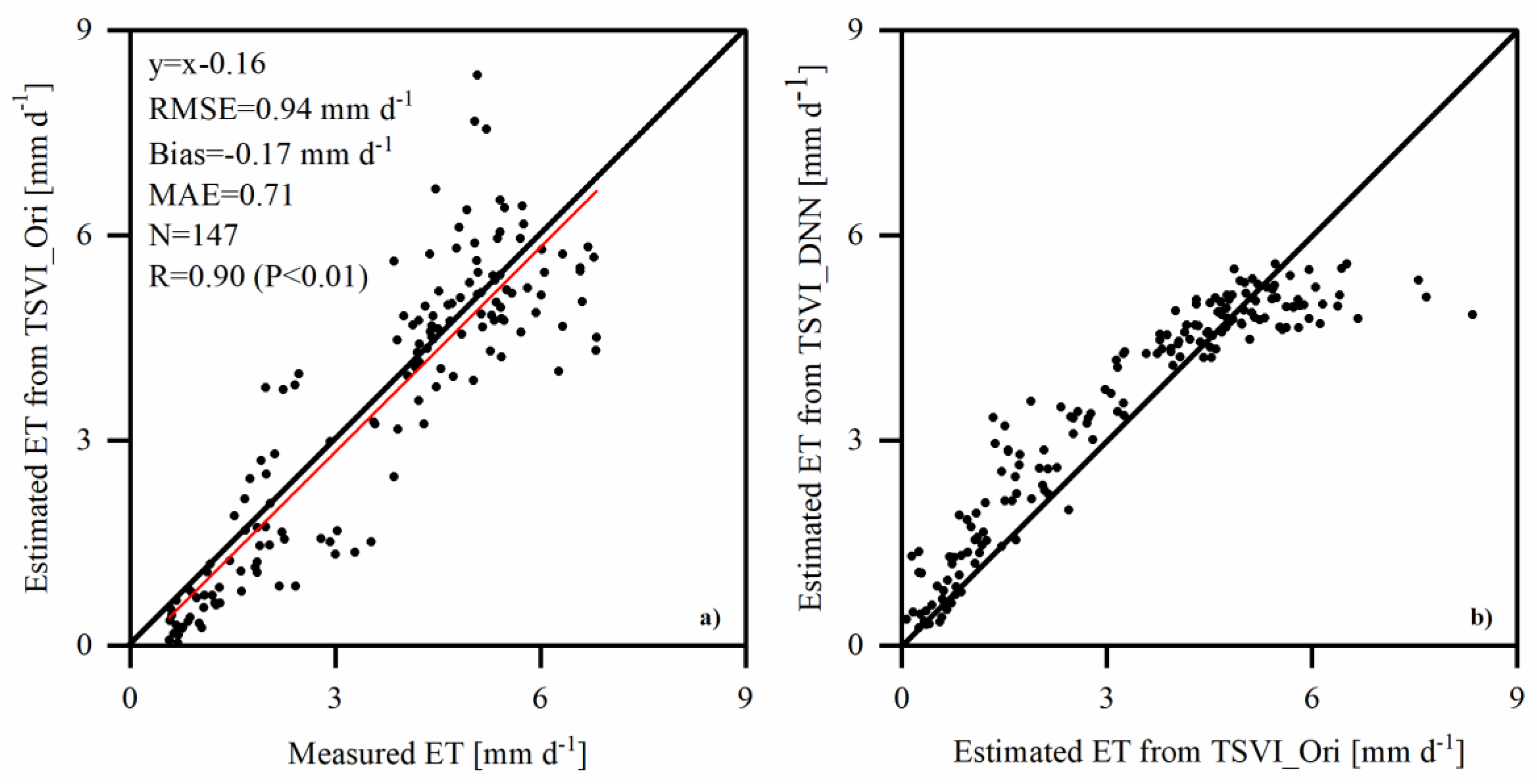
3.1. Comparison with the Original Ts-VI Triangle Model

Using three years of satellite observations over the study area, there were sufficient samples to train the DNN. Strict quality control was used to estimate ET using the TSVI_Ori model. Considering that the quality of the ET estimates from TSVI_Ori is critical in the DNN training process, we first evaluated it at YK station using three years of in situ measurements. Figure 4a reveals that a comparison of ET estimates from TSVI_Ori with in situ measurements is very close to 1:1 line, where an R of 0.9 (P < 0.01) indicates the model’s ability to capture the high variability in the data. Accuracy was acceptable with an RMSE of 0.94 mm d−1 and an MAD of 0.71 mm d−1. These results are comparable to those from previous studies of the Ts-VI triangle model [45]. Since bias was low, there was little underestimation of ET. When using satellite imagery there are other important issues to consider, such as their coarser spatial resolution, overpass frequency, the possibility of cloud cover presence at overpass time (imagery delivery time). These issues sometimes limit the effectiveness of the aforementioned methods for mapping daily ET at a very high resolution (crop fields) and on a regular basis for near real-time irrigation scheduling [21].
Approximately 6.8 × 10 5 high-quality ET estimates were obtained from the TSVI_Ori model for training the DNN, and 1.5 × 10 5 were randomly selected as validation data. ET estimates from the TSVI_DNN were compared to those from the TSVI_Ori ET during 2009–2011. As shown in Figure 4b, ET estimates from TSVI_DNN are highly consistent with estimates from TSVI_Ori at the YK station. Regional performance is also shown in Figure 5, revealing that, for the most part, the ET estimates from TSVI_DNN are highly consistent with the ET estimates from TSVI_Ori. The greatest difference between them is less than 1 mm d−1. We should state that the DNN configuration, to avoid overfitting, will not guarantee that the ET estimates from TSVI_DNN are the same as the ET estimates from TSVI_Ori, even though the traditional DNN has this ability. For example, the difference between outputs from the two models was relatively large when the ET estimates from TSVI_Ori were extremely high. This also indicates that there is a risk of missing extreme predictions using the TSVI_DNN model, which is a focus of future work.
The temporal coverage was improved from 16.1% with TSVI_Ori model to 67.1% with TSVI_DNN model during 2009–2011. Regardless of the surface covered by snow or the soil being frozen, TSVI_DNN is temporally continuous at the daily scale.
To show the spatial consistency between the TSVI_DNN and TSVI_Ori models, ET images on DOY 204 in 2009 are shown for both of them, for the both images had value in the growing season (Figure 6). The spatial pattern of ET estimates from the TSVI_DNN model was similar to that of TSVI_Ori, with ET decreasing from southeast to northwest. This ET spatial pattern is also consistent with those of previous studies [50,51,52]. In summary, the performance of both models during the period of overlap was highly consistent from point to regional scales, indicating that the DNN may have a high accuracy.

3.2. Comparison with MOD16 ET Product and In Situ Measurements

Although the TSVI_DNN model performs similarly to the TSVI_Ori model, its performance should also be evaluated against additional data. We first evaluated the TSVI_DNN against in situ measurements taken at the YK station during 2009–2011. The results show good agreement (Figure 7) between the results from the TSVI_DNN model and measured ET, where an R value of 0.9 (P < 0.01) indicates the model’s ability to capture high variability in the data. The RMSE, bias, and MAD are 0.86 mm d−1, −0.16 mm d−1, and 0.65 mm d−1, respectively, further showing high accuracy. These results are comparable to those between TSVI_DNN and TSVI_Ori. Compared with Figure 4a, these results have 562 samples, which is more than the 147 samples of TSVI_Ori. Considering that water resource management is always on the monthly or yearly scale, the bias is low enough to be compared with the water demand for maize of 4.3 mm d−1 [53]. Hence, it is reasonable to say that the TSVI_DNN model could be used in water resource management.
To further verify the results from our method, we chose to verify our results against the NASA official MOD16 ET version 6 product. Results from previous studies indicate that MOD16 ET products have varied widely and have shown good performance [10,38]. Hence, we selected it as a benchmark. The 500-m resolution original MOD16 ET was resampled to 0.01° spatial resolution, as mentioned previously. However, the temporal resolution of MOD16 ET is 8 days, which is longer than the 1-day estimates from in situ observations and our results. For comparison, we resampled ET estimates from the TSVI_DNN model and the in situ measurements of ET from 1 day to 8 days.
The time series of ET estimates from TSVI_DNN and MOD16 ET against in situ measured ET are shown in Figure 8. Both estimates can capture the annual variation shown by in situ ET measurements. However, MOD16 ET seriously underestimated measured values, while TSVI_DNN greatly reduced this underestimation. As shown in Table 2, when compared with MOD16 ET, the TSVI_DNN model reduced the RMSE with in situ measurements from 1.30 to 0.66 mm d−1, the bias from −0.89 to −0.23 mm d−1, and the MAD from 1.02 to 0.5 mm d−1. At the same time, R increased from 0.84 to 0.93. Thus, the accuracy (RMSE) of TSVI_DNN improved estimated ET by 49.2%, while also providing estimates closer to actual measurements, thereby reducing underestimation. We found that the latest version of MOD16 is of higher quality than the previous version (1 km, 8 day), which greatly underestimated ET at the YK station (data not shown) [52]. However, our results also show that there is still a lot of room for improvement in the MOD16 ET product.
As the scatterplot of regional ET estimates from TSVI_DNN vs. those from MODI 16 during 2009–2011 shows, the TSVI_DNN has a high correlation with the MOD 16 ET (R = 0.74, P < 0.01) (Figure 9a). However, the MOD16 underestimated ET more severely by about 1.06 mm d−1 than TSVI_DNN (Figure 9b). As an example, shown in Figure 9c,d, the spatial pattern of ET estimates from TSVI_DNN is similar to those from MOD16, where results also decreased from southeast to northwest.
Ideally, we expect that the TSVI_DNN model has a better extensible performance at different spatial and temporal scales. We therefore tested the TSVI_DNN model trained using 2009–2011 data to predict ET in 2012 and found that the quality of the variability and spatial pattern is comparable to that of the TSVI_Ori model (Figure 10). Meanwhile, two different scenarios were tested by training the TSVI_DNN using 2009–2011 data and predicting ET for 2012 vs. training the model and predicting ET for 2009–2012, comparing the results with the EC network measurements. Both methods showed similar results (Table 3) for both RMSE (1.24 vs. 1.20 mm d−1) and bias (−0.74 vs. −0.67 mm d−1). These metrics are comparable with the ET estimates from the TSVI_Ori model with an RMSE and bias of 1.13 mm d−1 and −0.72 mm d−1, respectively.

4. Discussion

4.1. Advantages of the TSVI_DNN Model

The most significant contribution of the TSVI_DNN model is filling the gaps in the ET estimates from the TSVI_Ori model using the DNN. It provided an applicable way to obtain temporally continuous daily ET over the arid area during the soil in unfrozen conditions, and the results show that the temporal coverage was significantly improved from 16.1% to 67.1% compared with the TSVI_Ori model. Meanwhile, the spatial pattern of TSVI_DNN is consistent with previous studies for the same area, which showed that spatial variation is small and ET is always high due to irrigation when using process-based and LST-based models [50,51,52].
In arid areas, actual ET is limited by the soil moisture, especially by the root zone soil moisture, and the irrigation events often introduce additional uncertainty. According to the mechanism of the TSVI_Ori model, the surface and root zone soil moisture have a great contribution to ET estimates from the TSVI_Ori model. Hence, the TSVI_DNN model provided a new way to extend the ET with the contribution of soil moisture to different spatio-temporal scale with the help of DNN. However, other mechanism models either limited by the coarse resolution of surface soil moisture product or by a lack of fine-resolution and reliable root zone soil moisture, and using atmospheric vapor pressure deficit as a surrogate might introduce additional uncertainty due to its low spatial variation [11,54,55].
In addition, the TSVI_DNN model relies on the inputs from remotely sensed and forcing data, but does not need ground data. This was another main difference from the widely used crop coefficient based Penman-Monteith method, where the crop coefficient is obtained through field experiment and varies during vegetation developing stages [56]. Moreover, it is also different from the ground data driven machine learning methods [24].
What is more, this study used the DNN to establish relationships between daily ET estimates from the Ts-VI triangle model and reference data and then obtain temporally continuous daily ET by overcoming the issue of gaps on cloudy days. The DNN has a stronger relationship-mining ability than more traditional neural networks, especially for large training datasets. When increasing the size of the training dataset, the established relationship becomes more stable.

4.2. Limitations of the TSVI_DNN Model

A number of limitations of the Ts-VI triangle model should be stated to further improve the quality of TSVI_DNN in the future. (1) The error in daily ET estimates used as training data from the Ts-VI triangle model has at least two components: errors in the Ts-VI triangle model and errors in the scaling/transforming process. In this study, we limited the clear-sky conditions to relative stable weather based on the quality of LST and precipitation. The total error (RMSE) of the daily ET estimates of 0.94 mm d−1 suggests that this method was effective. (2) Several factors can reduce the performance of the Ts-VI triangle model. For example, heavy rainfall on the last day might lead to an inaccurate determination of the dry and wet edges [45]. Although there are a number of papers indicating that the coefficient of the P-T equation equals 1.26, values ranging from 1.0 to 1.5 have also been reported [1,45,57]. (3) There are at least five methods that can be used to transform instantaneous remote sensing latent heat flux or evaporation observations to daily estimates [18,21]. Most methods, such as the reference ET-based method, need more instantaneous information, which is difficult to obtain at satellite overpass time. Hence, in this study, we used the simple EF-based method. Despite its limitations, the Ts_VI triangle model is a good choice to estimate ET estimation based on results from a number of published studies. Independent validation in this study also proves that the use of the Ts_VI triangle model can generate acceptable estimates of daily ET.
Other limitations include the low reliability and coarse resolution forcing data from the global land model, e.g., GLDAS [58]. In this study, data correction by the weather station observations and downscaling by empirical methods to improve the spatial resolution to 0.01° can reduce this error to a degree [42]. This might be a compromise compared with the complex dynamic downscaling method using the weather research and forecasting model (WRF) at mesoscale [59].
Other LST-based ET model estimates can also be used to train the DNN. For example, the SEBS and Norman-95 (N95) models are widely used in regional ET estimates using remotely sensed LST [13,60]. They have similar advantages in that both have reasonably favorable accuracy and direct monitoring, while their disadvantage is in being constrained by clouds because of the sensitivity of LST. Our results using the Ts-VI triangle model present a satisfactory case. It should be noted that different ET models may have distinguishable differences. Quality control is critical in this extension of the application, where quality is more important than the number of datapoints. Meanwhile, DNN still has less ability to capture extreme values (very high and low ET) than traditional neural networks. Future studies will explore methods to improve this DNN.

5. Conclusions

LST-based ET models are confronted with difficulties in estimating temporally continuous daily actual ET. In this study, we developed a gap-filling algorithm using DNN for the Ts-VI triangle model to obtain temporally continuous daily actual ET in an arid area of China. High-quality discontinuous daily ET was obtained from the TSVI_Ori ET model under clear-sky condition using high-quality LST observations. We took advantage of these high-quality ET estimates, along with meteorological forcing data, to train the DNN. Finally, the trained TSVI_DNN model was used to estimate temporally continuous daily actual ET at the regional scale in an arid area. We found that: (1) ET estimates from the TSVI_DNN model showed the ability to capture the high variability in ET with an R of 0.9. The results were highly accurate with an RMSE of 0.86 mm d−1 and an MAD of 0.65 mm d−1. The bias towards underestimation was low (with a bias of −0.16 mm d−1); (2) the ET estimates from TSVI_DNN are highly consistent with the ET estimates from the TSVI_Ori model, although it was necessary to avoid the overfitting of the DNN by adopting methods designed for that task; (3) compared with the NASA official MOD16 ET version 6 product, the accuracy (RMSE) of TSVI_DNN improved estimates by 49.2%. The in situ comparison with measurements and intercomparison with the MOD16 product showed that TSVI_DNN demonstrated outstanding performance. In summary, due to the high non-stationarity and non-linearity characteristics of the ET process, the DNN provides a practical alternative to estimating temporally continuous daily ET based on the LST-based ET model.

Author Contributions

Conceptualization, methodology and analysis, Y.C.; software, Y.C. and S.M.; validation and visualization, Z.Y., X.C., and Z.L.; writing—original draft preparation, Y.C.; writing—review and editing, W.F. and Y.H. All authors have read and agreed to the published version of the manuscript.

Funding

This study was financially supported by the Key R&D Program of the Ministry of Science and Technology, China (Grant No. 2017YFE0122400, No. 2018YFC1506504 and No. 2016YFC0500205) and the National Science Foundation of China (Grant No. 41901348), and the Strategic Priority Research Program of the Chinese Academy of Sciences (Grant No. XDA19030203).

Acknowledgments

We thank three anonymous reviewers for their valuable comments to improve this manuscript.

Conflicts of Interest

The authors declare no conflict of interest.

References

  1. Wang, K.C.; Dickinson, R.E. A Review of Global Terrestrial Evapotranspiration: Observation, Modeling, Climatology, And Climatic Variability. Rev. Geophys. 2012, 50. [Google Scholar] [CrossRef]
  2. Sacks, W.J.; Kucharik, C.J. Crop management and phenology trends in the U.S. Corn Belt: Impacts on yields, evapotranspiration and energy balance. Agric. For. Meteorol. 2011, 151, 882–894. [Google Scholar] [CrossRef]
  3. Rhenals, A.E.; Bras, R.L.J.W.R.R. The irrigation scheduling problem and evapotranspiration uncertainty. Water Resour. Res. 1981, 17, 1328–1338. [Google Scholar] [CrossRef]
  4. Ma, W.; Hafeez, M.; Ishikawa, H. Evaluation of SEBS for estimation of actual evapotranspiration using ASTER satellite data for irrigation areas of Australia. Theor. Appl. Climatol. 2013, 112, 609–616. [Google Scholar] [CrossRef]
  5. Odeh, T.; Mohammad, A.H.; Hussein, H.; Ismail, M.; Almomani, T. Over-pumping of groundwater in Irbid governorate, northern Jordan: A conceptual model to analyze the effects of urbanization and agricultural activities on groundwater levels and salinity. Environ. Earth Sci. 2019, 78, 103766. [Google Scholar] [CrossRef] [Green Version]
  6. Mohammad, A.H.; Jung, H.C.; Odeh, T.; Bhuiyan, C.; Hussein, H. Understanding the impact of droughts in the Yarmouk Basin, Jordan: Monitoring droughts through meteorological and hydrological drought indices. Arab. J. Geosci. 2018, 11, 103. [Google Scholar] [CrossRef] [Green Version]
  7. Riad, P.; Graefe, S.; Hussein, H.; Buerkert, A. Landscape transformation processes in two large and two small cities in Egypt and Jordan over the last five decades using remote sensing data. Landsc. Urban Plan. 2020, 197, 103766. [Google Scholar] [CrossRef]
  8. Jiang, L.; Islam, S. A methodology for estimation of surface evapotranspiration over large areas using remote sensing observations. Geophys. Res. Lett. 1999, 26, 2773–2776. [Google Scholar] [CrossRef] [Green Version]
  9. Monteith, J.L. Evaporation and environment. Symp. Soc. Exp. Biol. 1965, 19, 205–223. [Google Scholar]
  10. Mu, Q.Z.; Zhao, M.S.; Running, S.W. Improvements to a MODIS global terrestrial evapotranspiration algorithm. Remote Sens. Environ. 2011, 115, 1781–1800. [Google Scholar] [CrossRef]
  11. Zhang, K.; Kimball, J.S.; Running, S.W.J.W.W. A review of remote sensing based actual evapotranspiration estimation. Water 2016, 3, 834–853. [Google Scholar] [CrossRef]
  12. Bastiaanssen, W.; Menenti, M.; Feddes, R.; Holtslag, A. A remote sensing surface energy balance algorithm for land (SEBAL). 1. Formulation. J. Hydrol. 1998, 212, 198–212. [Google Scholar] [CrossRef]
  13. Su, Z. The Surface Energy Balance System (SEBS) for estimation of turbulent heat fluxes. Hydrol. Earth Syst. Sci. 2002, 6, 85–99. [Google Scholar] [CrossRef]
  14. Stewart, J.B.; Kustas, W.P.; Humes, K.S.; Nichols, W.D.; Moran, M.S.; Debruin, H.A.R. Sensible Heat-Flux Radiometric Surface-Temperature Relationship for 8 Semiarid Areas. J. Appl. Meteorol. 1994, 33, 1110–1117. [Google Scholar] [CrossRef] [Green Version]
  15. Jiang, L.; Islam, S. Estimation of surface evaporation map over southern Great Plains using remote sensing data. Water Resour. Res. 2001, 37, 329–340. [Google Scholar] [CrossRef] [Green Version]
  16. Tang, R.; Li, Z.-L.; Chen, K.-S. Validating MODIS-derived land surface evapotranspiration with in situ measurements at two AmeriFlux sites in a semiarid region. J. Geophys. Res. Space Phys. 2011, 116, 116. [Google Scholar] [CrossRef] [Green Version]
  17. Zhu, W.; Jia, S.; Lv, A. A Universal Ts-VI Triangle Method for the Continuous Retrieval of Evaporative Fraction From MODIS Products. J. Geophys. Res. Atmos. 2017, 122, 206–210. [Google Scholar] [CrossRef]
  18. Colaizzi, P.D.; Evett, S.R.; Howell, T.A.; Tolk, J.A. Comparison of Five Models to Scale Daily Evapotranspiration from One-Time-of-Day Measurements. T. Asabe 2006, 49, 1409–1417. [Google Scholar] [CrossRef]
  19. Sugita, M.; Brutsaert, W. Daily evaporation over a region from lower boundary layer profiles measured with radiosondes. Water Resour. Res. 1991, 27, 747–752. [Google Scholar] [CrossRef]
  20. Jackson, R.; Hatfield, J.; Reginato, R.; Idso, S.; Pinter, P., Jr. Estimation of daily evapotranspiration from one time-of-day measurements. Agric. Water Manag. 1983, 7, 351–362. [Google Scholar] [CrossRef]
  21. Chávez, J.L.; Neale, C.M.U.; Prueger, J.H.; Kustas, W.P. Daily evapotranspiration estimates from extrapolating instantaneous airborne remote sensing ET values. Irrig. Sci. 2008, 27, 67–81. [Google Scholar] [CrossRef]
  22. Anderson, M.C.; Norman, J.M.; Mecikalski, J.R.; Otkin, J.A.; Kustas, W.P. A climatological study of evapotranspiration and moisture stress across the continental United States based on thermal remote sensing: 1. Model Formul. 2007, 112. [Google Scholar] [CrossRef]
  23. He, C.; Yang, D. Remote sensing based continuous estimation of regional evapotranspiration by improved SEBS model. SPIE Asia-Pac. Remote Sens. 2012, 8524, 85240. [Google Scholar]
  24. Chen, Y.; Xia, J.; Liang, S.; Feng, J.; Fisher, J.B.; Li, X.; Li, X.; Liu, S.; Ma, Z.; Miyata, A.; et al. Comparison of satellite-based evapotranspiration models over terrestrial ecosystems in China. Remote Sens. Environ. 2014, 140, 279–293. [Google Scholar] [CrossRef]
  25. Dou, X.; Yang, Y. Evapotranspiration estimation using four different machine learning approaches in different terrestrial ecosystems. Comput. Electron. Agric. 2018, 148, 95–106. [Google Scholar] [CrossRef]
  26. Torres, A.F.; Walker, W.R.; McKee, M. Forecasting daily potential evapotranspiration using machine learning and limited climatic data. Agric. Water Manag. 2011, 98, 553–562. [Google Scholar] [CrossRef]
  27. Cui, Y.; Long, D.; Hong, Y.; Zeng, C.; Zhou, J.; Han, Z.; Liu, R.; Wan, W. Validation and reconstruction of FY-3B/MWRI soil moisture using an artificial neural network based on reconstructed MODIS optical products over the Tibetan Plateau. J. Hydrol. 2016, 543, 242–254. [Google Scholar] [CrossRef]
  28. Yoshua, B. Learning Deep Architectures for AI; Now: Delft, The Netherlands, 2009; p. 1. [Google Scholar]
  29. Fang, K.; Shen, C.; Kifer, D.; Xiao, Y.J.G.R.L. Prolongation of SMAP to Spatio-temporally Seamless Coverage of Continental US Using a Deep Learning Neural Network. Geophys. Res. Lett. 2017, 14, 11–30. [Google Scholar]
  30. Tao, Y.; Gao, X.; Hsu, K.; Sorooshian, S.; Ihler, A. A Deep Neural Network Modeling Framework to Reduce Bias in Satellite Precipitation Products. J. Hydrometeorol. 2016, 17, 931–945. [Google Scholar] [CrossRef]
  31. Cui, Y.; Chen, X.; Gao, J.; Yan, B.; Tang, G.; Hong, Y.J.B.E.D. Global water cycle and remote sensing big data: Overview, challenge, and opportunities. Big Earth Data 2018, 2, 282–297. [Google Scholar] [CrossRef]
  32. Li, X.; Li, X.W.; Li, Z.Y.; Ma, M.G.; Wang, J.; Xiao, Q.; Liu, Q.; Che, T.; Chen, E.X.; Yan, G.J.; et al. Watershed Allied Telemetry Experimental Research. J. Geophys. Res.-Atmos. 2009, 114, 114. [Google Scholar] [CrossRef] [Green Version]
  33. Li, X.; Cheng, G.D.; Liu, S.M.; Xiao, Q.; Ma, M.G.; Jin, R.; Che, T.; Liu, Q.H.; Wang, W.Z.; Qi, Y.; et al. Heihe Watershed Allied Telemetry Experimental Research (HiWATER): Scientific Objectives and Experimental Design. Bull. Am. Meteorol. Soc. 2013, 94, 1145–1160. [Google Scholar] [CrossRef]
  34. Liu, S.M.; Xu, Z.W.; Wang, W.Z.; Jia, Z.Z.; Zhu, M.J.; Bai, J.; Wang, J.M. A comparison of eddy-covariance and large aperture scintillometer measurements with respect to the energy balance closure problem. Hydrol. Earth Syst. Sci. 2011, 15, 1291–1306. [Google Scholar] [CrossRef] [Green Version]
  35. Yan, K.; Park, T.; Yan, G.; Chen, C.; Yang, B.; Liu, Z.; Nemani, R.; Knyazikhin, Y.; Myneni, R. Evaluation of MODIS LAI/FPAR Product Collection 6. Part 1: Consistency and Improvements. Remote Sens. 2016, 8, 359. [Google Scholar] [CrossRef] [Green Version]
  36. Jia, L.; Shang, H.; Hu, G.; Menenti, M. Phenological response of vegetation to upstream river flow in the Heihe Rive basin by time series analysis of MODIS data. Hydrol. Earth Syst. Sci. 2011, 15, 1047–1064. [Google Scholar] [CrossRef] [Green Version]
  37. Liu, Q.; Wang, L.Z.; Qu, Y.; Liu, N.F.; Liu, S.H.; Tang, H.R.; Liang, S.L. Preliminary evaluation of the long-term GLASS albedo product. Int. J. Digit. Earth 2013, 6, 69–95. [Google Scholar] [CrossRef]
  38. Mu, Q.; Heinsch, F.A.; Zhao, M.; Running, S.W. Development of a global evapotranspiration algorithm based on MODIS and global meteorology data. Remote Sens. Environ. 2007, 111, 519–536. [Google Scholar] [CrossRef]
  39. Liu, Y.Y.; Parinussa, R.M.; Dorigo, W.A.; De Jeu, R.A.M.; Wagner, W.; van Dijk, A.I.J.M.; McCabe, M.F.; Evans, J.P. Developing an improved soil moisture dataset by blending passive and active microwave satellite-based retrievals. Hydrol. Earth Syst. Sci. 2011, 15, 425–436. [Google Scholar] [CrossRef] [Green Version]
  40. Cui, Y.; Zeng, C.; Zhou, J.; Xie, H.; Wan, W.; Hu, L.; Xiong, W.; Chen, X.; Fan, W.; Hong, Y. A spatio-temporal continuous soil moisture dataset over the Tibet Plateau from 2002 to 2015. Sci. Data 2019, 6, 247. [Google Scholar] [CrossRef] [Green Version]
  41. Chen, Y.Y.; Yang, K.; He, J.; Qin, J.; Shi, J.C.; Du, J.Y.; He, Q. Improving land surface temperature modeling for dry land of China. J. Geophys Res. Atmos. 2011, 116. [Google Scholar] [CrossRef]
  42. He, J.; Yang, K.; Tang, W.; Lu, H.; Qin, J.; Chen, Y.; Li, X. The first high-resolution meteorological forcing dataset for land process studies over China. Sci. Data 2020, 7, 25. [Google Scholar] [CrossRef] [Green Version]
  43. Gao, Y.C.; Long, D.; Li, Z.L. Estimation of daily actual evapotranspiration from remotely sensed data under complex terrain over the upper Chao river basin in North China. Int. J. Remote Sens. 2008, 29, 3295–3315. [Google Scholar] [CrossRef]
  44. Stahl, K.; Moore, R.D.; Floyer, J.A.; Asplin, M.G.; McKendry, I.G. Comparison of approaches for spatial interpolation of daily air temperature in a large region with complex topography and highly variable station density. Agric. For. Meteorol. 2006, 139, 224–236. [Google Scholar] [CrossRef]
  45. Tang, R.; Li, Z.; Tang, B. An application of the T-s-VI triangle method with enhanced edges determination for evapotranspiration estimation from MODIS data in and and semi-arid regions: Implementation and validation. Remote Sens. Environ. 2010, 114, 540–551. [Google Scholar] [CrossRef]
  46. Nichols, W.E.; Cuenca, R.H. Evaluation of the evaporative fraction for parameterization of the surface energy balance. Water Resour. Res. 1993, 29, 3681–3690. [Google Scholar] [CrossRef]
  47. Nair, V.; Hinton, G.E. Rectified Linear Units Improve Restricted Boltzmann Machines Vinod Nair. In Proceedings of the 27th International Conference on Machine Learning (ICML-10), Haifa, Israel, 21–24 June 2010. [Google Scholar]
  48. Kingma, D.; Ba, J. Adam: A Method for Stochastic Optimization. arXiv 2014, arXiv:1412.6980. [Google Scholar]
  49. Cui, Y.; Chen, X.; Xiong, W.; He, L.; Lv, F.; Fan, W.; Luo, Z.; Hong, Y. A Soil Moisture Spatial and Temporal Resolution Improving Algorithm Based on Multi-Source Remote Sensing Data and GRNN Model. Remote Sens. 2020, 12, 455. [Google Scholar] [CrossRef] [Green Version]
  50. Li, X.; Lu, L.; Yang, W.; Cheng, G. Estimation of evapotranspiration in an arid region by remote sensing—A case study in the middle reaches of the Heihe River Basin. Int. J. Appl. Earth Obs. 2012, 17, 85–93. [Google Scholar] [CrossRef]
  51. Li, Y.; Huang, C.; Hou, J.; Gu, J.; Zhu, G.; Li, X.J.A.; Meteorology, F. Mapping daily evapotranspiration based on spatiotemporal fusion of ASTER and MODIS images over irrigated agricultural areas in the Heihe River Basin, Northwest China. Agric. For. Meteorol. 2017, 244, 82–97. [Google Scholar] [CrossRef]
  52. Hu, G.; Li, J. Monitoring of Evapotranspiration in a Semi-Arid Inland River Basin by Combining Microwave and Optical Remote Sensing Observations. Remote Sens. 2015, 7, 3056–3087. [Google Scholar] [CrossRef] [Green Version]
  53. Zhao, W.; Liu, B.; Zhang, Z. Water requirements of maize in the middle Heihe River basin, China. Agric. Water Manag. 2010, 97, 215–223. [Google Scholar] [CrossRef]
  54. Entekhabi, D.; Njoku, E.G.; Neill, P.E.O.; Kellogg, K.H.; Crow, W.T.; Edelstein, W.N.; Entin, J.K.; Goodman, S.D.; Jackson, T.J.; Johnson, J.; et al. The Soil Moisture Active Passive (SMAP) Mission. Proc. IEEE 2010, 98, 704–716. [Google Scholar] [CrossRef]
  55. Martens, B.; Miralles, D.G.; Lievens, H.; van der Schalie, R.; de Jeu, R.A.M.; Fernández-Prieto, D.; Beck, H.E.; Dorigo, W.A.; Verhoest, N.E.C. GLEAM v3: Satellite-based land evaporation and root-zone soil moisture. Geosci. Model. Dev. 2017, 10, 1903–1925. [Google Scholar] [CrossRef] [Green Version]
  56. Shen, Y.; Li, S.; Chen, Y.; Qi, Y.; Zhang, S. Estimation of regional irrigation water requirement and water supply risk in the arid region of Northwestern China 1989–2010. Agric. Water Manag. 2013, 128, 55–64. [Google Scholar] [CrossRef]
  57. Abtew, W. Evapotranspiration measurements and modeling for three wetland systems in south florida1. JAWRA 1996, 32, 465–473. [Google Scholar] [CrossRef]
  58. Rodell, M.; Houser, P.R.; Jambor, U.; Gottschalck, J.; Mitchell, K.; Meng, C.J.; Arsenault, K.; Cosgrove, B.; Radakovich, J.; Bosilovich, M.; et al. The global land data assimilation system. Bull. Am. Meteorol. Soc. 2004, 85, 381–394. [Google Scholar] [CrossRef] [Green Version]
  59. Pan, X.D.; Li, X.; Shi, X.K.; Han, X.J.; Luo, L.H.; Wang, L.X. Dynamic downscaling of near-surface air temperature at the basin scale using WRF-a case study in the Heihe River Basin, China. Front. Earth Sci.-Prcact. 2012, 6, 314–323. [Google Scholar] [CrossRef]
  60. Norman, J.M.; Kustas, W.P.; Humes, K.S. Source Approach for Estimating Soil And Vegetation Energy Fluxes In Observations Of Directional Radiometric Surface-Temperature. Agric. For. Meteorol. 1995, 77, 263–293. [Google Scholar] [CrossRef]
Figure 1. Study area and location of eddy covariance (EC) stations. (a) A land cover map of the study area; (b) the location of EC stations on the Normalized Difference Vegetation Index (NDVI) map (DOY = 192). YK = Yingke station.
Remotesensing 12 01121 g001
Figure 2. Flowchart for obtaining temporal continuous daily actual evapotranspiration based on the Ts-VI triangle method and the deep the neural network. Where WS: wind speed; AT: air temperature; RH: relative humidity; AP: air pressure; DSR: downward shortwave radiation; DLR: downward longwave radiation; SM: soil moisture; Ts-VI: surface temperature-vegetation index; DNN: deep neural network.
Remotesensing 12 01121 g002
Figure 3. Structure of the DNN used in the study.
Remotesensing 12 01121 g003
Figure 4. Comparison of evapotranspiration (ET) estimates from the TSVI_DNN and TSVI_Ori models at the YK station during 2009–2011. (a) A scatterplot of ET estimates from the TSVI_Ori model vs. measured ET; (b) a scatterplot of ET estimates from TSVI_Ori vs. TSVI_DNN.
Remotesensing 12 01121 g004
Figure 5. Comparison of ET estimates from the TSVI_DNN and TSVI_Ori model on the regional scale. (a) A scatterplot of regional ET estimates from TSVI_DNN vs. those from TSVI_Ori; (b) a histogram of the difference between ET estimates from the TSVI_DNN and TSVI_Ori models.
Remotesensing 12 01121 g005
Figure 6. Spatial pattern of ET estimates from the TSVI_DNN and TSVI_Ori models on DOY 204 in 2009. (a) ET estimates from the TSVI_Ori model; (b) ET estimates from the TSVI_DNN model. Units: mm d−1.
Remotesensing 12 01121 g006
Figure 7. Scatterplot of ET estimates from the TSVI_DNN compared to the in situ measurements of ET.
Remotesensing 12 01121 g007
Figure 8. Time series of ET estimates from the TSVI_DNN model and the MOD16 ET product, as compared to in situ measurements at the YK station during 2009–2011.
Remotesensing 12 01121 g008
Figure 9. Regional difference and spatial pattern of ET estimates from TSVI_DNN and MOD16 ET. (a) A scatterplot of regional ET estimates from TSVI_DNN vs. those from MODI 16 during 2009–2011; (b) a histogram of the difference between ET estimates from the TSVI_DNN model and MOD 16 during 2009–2011. (c) and (d) are the spatial pattern of ET estimates from the TSVI_DNN model and from the MOD16 on DOY 201~208 in 2009, respectively.
Remotesensing 12 01121 g009
Figure 10. Spatial distribution of ET estimates from TSVI_DNN (b,d,f) trained during 2009–2011 and TSVI_Ori (a,c,e) on DOY 150, 214, and 283 in 2012 from top to bottom, respectively. Unit: mm d−1.
Remotesensing 12 01121 g010
Table 1. Remotely sensed and meteorological forcing datasets used in this study. The variables in regular font are used in the Ts-VI triangle model, while the variables in italics are used in the deep neural network (DNN). Where LST: land surface temperature; NDVI: normalized difference vegetation index; SM: soil moisture; WS: wind speed; AT: air temperature; RH: relative humidity; AP: air pressure; DSR: downward shortwave radiation; DLR: downward longwave radiation; ET: evapotranspiration.
VariableSourceSpatial ResolutionTemporal ResolutionTime Available
LSTMOD11A11 km1-day2009–2012
NDVIMOD13A21 km8-day2009–2012
AlbedoGLASS1 km8-day2009–2012
SMESA ECV0.25°1-day2009–2012
WSDAMCTM0.1°3-h2009–2012
ATDAMCTM0.1°3-h2009–2012
RHDAMCTM0.1°3-h2009–2012
APDAMCTM0.1°3-h2009–2012
DSRDAMCTM0.1°3-h2009–2012
DLRDAMCTM0.1°3-h2009–2012
ETMOD16A2500 m8-day2009–2011
Land coverMOD12Q1 km1-year2009
PrecipitationDAMCTM0.1°3-h2009–2012
Table 2. Error metrics of ET estimates from the TSVI_DNN model and MOD16 ET product as compared to in situ measurements at the YK station during 2009–2011, including R (correlation coefficient), RMSE (root mean square error, mm d−1), bias (mean bias, mm d−1), MAD (Mean Absolute Deviation, mm d−1), and N (the number of samples).
ProductRRMSEBiasMADN
TSVI_DNN0.930.66−0.230.5049
MOD 160.841.30−0.891.0252
Table 3. Error metrics of ET estimates from TSVI_Ori and TSVI_DNN compared with measurements from the EC network in 2012 for two different scenarios: training using 2009–2011 data to predict ET in 2012 vs. training and predicting ET for 2009–2012, including R (correlation coefficient), RMSE (root mean square error, mm d−1), bias (mean bias, mm d−1), MAD (Mean Absolute Deviation, mm d−1), and N (the number of samples).
SceneRRMSEBiasMADN
Training during 2009–2011 and predicting for 20120.741.24−0.741.01381
Training and predicting for 2009–20120.741.20−0.670.93381
TSVI_Ori0.821.13−0.720.93127

