On-the-Fly Camera and Lidar Calibration

Abstract

Sensor fusion is one of the main challenges in self driving and robotics applications. In this paper we propose an automatic, online and target-less camera-Lidar extrinsic calibration approach. We adopt a structure from motion (SfM) method to generate 3D point clouds from the camera data which can be matched to the Lidar point clouds; thus, we address the extrinsic calibration problem as a registration task in the 3D domain. The core step of the approach is a two-stage transformation estimation: First, we introduce an object level coarse alignment algorithm operating in the Hough space to transform the SfM-based and the Lidar point clouds into a common coordinate system. Thereafter, we apply a control point based nonrigid transformation refinement step to register the point clouds more precisely. Finally, we calculate the correspondences between the 3D Lidar points and the pixels in the 2D camera domain. We evaluated the method in various real-life traffic scenarios in Budapest, Hungary. The results show that our proposed extrinsic calibration approach is able to provide accurate and robust parameter settings on-the-fly.

1. Introduction

Nowadays, state-of-the-art autonomous systems rely on wide range of sensors for environment perception such as optical cameras, radars and Lidars, therefore efficient sensor fusion is a highly focused research topic in the fields of self-driving vehicles and robotics. Though the resolution and the operation speed of these sensors have significantly improved in recent years, and their prices have become affordable in mass production, their measurements have highly diverse characteristics, which makes the efficient exploitation of the multimodal data challenging. While real time Lidars, such as Velodyne’s rotating multi-beam (RMB) sensors provide accurate 3D geometric information with relatively low vertical resolution, optical cameras capture high resolution and high quality image sequences enabling to perceive low level details from the scene. A common problem with optical cameras is that extreme lighting conditions (such as dark, or strong sunlight) largely influence the captured image data, while Lidars are able to provide reliable information much less depending on external illumination and weather conditions. On the other hand, by simultaneous utilization of Lidar and camera sensors, accurate depth with detailed texture and color information can be obtained in parallel from the scenes.

Accurate Lidar and camera calibration is an essential step to implement robust data fusion, thus, related issues are extensively studied in the literature [1,2,3]. Existing calibration techniques can be grouped based on a variety of aspects [1]: based on the level of user interaction they can be semi- or fully automatic, methodologically we can distinguish target-based and target-less approaches, and in the term of operational requirements offline and online approaches can be defined (see Section 2).

In this paper, we propose a new fully automatic and target-less extrinsic calibration approach between a camera and a rotating multi-beam (RMB) Lidar mounted on a moving car. Our new method consists of two main steps: an object level matching algorithm performing a coarse alignment of the camera and Lidar data, and a fine alignment step which implements a control point based point level registration refinement. Our method relies on only the raw camera and Lidar sensor streams without using any external Global Navigation Satellite System (GNSS) or Inertial Measurement Unit (IMU) sensors. Moreover, it is able to automatically calculate the extrinsic calibration parameters between the Lidar and camera sensors on-the-fly which means we only have to mount the sensors on the top of the vehicle and start driving in a typical urban environment. In the object level coarse alignment stage, we first obtain a synthesized 3D environment model from the consecutive camera images using a Structure from Motion (SfM) pipeline then we extract object candidates from both the generated model and the Lidar point cloud. Since the density of the Lidar point cloud quickly decreases as a function of the distance from the sensor, we only consider key-points extracted from robustly observable landmark objects for registration. In the first stage, the object-based coarse alignment step searches for a rigid-body transformation, assuming that both the Lidar and the SfM point clouds accurately reflect the observed 3D scene. However in practice various mismatches and inaccurate scaling effects may occur during the SfM process; furthermore, due to the movement of the scanning platform ellipsoid-shape distortions can also appear in the Lidar point cloud. In the second stage, in order to compensate for these distortions of the point clouds, we fit a Non-Uniform Rational B-Spline (NURBS) curve to the extracted registration landmark key-points, which step enables to flexibly form the global shape of the point clouds.

The outline of the paper is as follows: in Section 2 we give a detailed insight into the literature of camera-Lidar calibration, Section 3 introduces the proposed method and finally in Section 4 we quantitatively and qualitatively evaluate our fully automatic and target-less approach in real urban environment and we compare the performance of the proposed method against state-of-the-art target-based [2] and target-less calibration techniques [4,5].

A preliminary stage of the proposed method has been introduced in [6,7]. This paper presents a more elaborated model, with a significant extension using a curve-based non-rigid transformation component, while we also provide here more extensive evaluation and comparison against several reference techniques.

2. Related Works

As mentioned above, extrinsic calibration approaches can be methodologically divided into two main categories: target-based and target-less methods.

As their main characteristics, target-based methods use special calibration targets such as 3D boxes [2], checkerboard patterns [8], a simple printed circle [9], or a unique polygonal planar board [10] during the calibration process. In the level of user interactions, we can subdivide target-based methods into semi-automatic and fully-automatic techniques. Semi-automatic methods may consist of many manual steps, such as moving the calibration patterns in different positions, manually localizing the target objects both in the Lidar and in the camera frames, and adjusting the parameters of the calibration algorithms. Though semi-automatic methods may yield very accurate calibration, these approaches are very time consuming and the calibration results highly depend on the skills of the operators. Moreover, even a well calibrated system may periodically need re-calibration due to artifacts caused by vibration and sensor deformation effects.

Fully-automatic target-based methods attempt to automatically detect previously defined target objects, then they extract and match features without user intervention: Velas et al. [11] detect circular holes on planar targets, Park et al. [10] calibrate Lidar and camera by using white homogeneous target objects, Geiger et al. [8] use corner detectors on multiple checkerboards and Rodriguez et. al. [12] detect ellipse patterns automatically. Though the mentioned approaches do not need operator interactions, they still rely on the presence of calibration targets, which often should be arranged in complex setups (i.e., [8] uses 12 checkerboards). Furthermore, during the calibration both the platform and the targets must be motionless.

On the contrary, target-less approaches rely on features extracted from the observed scene without using any calibration objects. Some of these methods use motion-based [13,14,15] information to calibrate the Lidar and camera, while alternative techniques [1,5] attempt to minimize the calibration errors using only static features.

Among motion-based approaches, Huang and Stachniss [14] improve the accuracy of extrinsic calibration by the estimation of the motion errors, Shiu and Ahmad [13] approximate the relative motion parameters between the consecutive frames, and Shi et al. [16] calculate sensor motion by jointly minimizing the projection error between the Lidar and the camera residuals. These methods estimate first the trajectories of the camera and Lidar sensors either by visual odometry and scan matching techniques, or by exploiting IMU and GNSS measurements. Thereafter they match the recorded camera and Lidar measurement sequences assuming that the sensors are rigidly mounted to the platform. However, the accuracy of these techniques strongly depends on the performance of trajectory estimation, which may suffer from visual featureless regions, low resolution scans [17], lack of hardware trigger based synchronization between the camera and the Lidar [16], or urban scenes without sufficient GPS coverage.

We continue the discussion with single frame target-less and feature-based methods. Moghadam et al. [5] attempt to detect correspondences by extracting lines both from the 3D Lidar point cloud and the 2D image data. While this method proved to be efficient in indoor environments, it requires a large number of line correspondences, a condition which cannot be often satisfied in outdoor scenes. A mutual information based approach has been introduced in [18] to calibrate different range sensors with cameras. Pandey et al. [1] attempt to maximize the mutual information using the camera’s grayscale pixel intensities and the Lidar reflectivity values. Based on Lidar reflectivity values and grayscale images Napier et al. [19] minimize the correlation error between the Lidar and the camera frames. Scaramuzza et al. [4] introduce a new data representation called the Bearing Angle image (BA) which is generated from the Lidar’s range measurements. Using conventional image processing operations, the method searches for correspondences between the BA and the camera image. As a limitation, target-less feature-based methods require a reasonable initial transformation estimation between the different sensors measurement [16], and mutual information based matching is sensitive to inhomogeneous point cloud inputs and illumination artifacts, which are frequently occurring problems when using RMB Lidars [1].

In this paper, we propose a two-stage fully automatic target-less camera-Lidar calibration method, which requires neither hardware trigger based sensor synchronization, nor accurate self-localization, trajectory estimation or simultaneous localization and mapping (SLAM) implementation. It can also be used by experimental platforms with ad-hoc sensor configurations, since after mounting the sensors to the car’s roof top, all registration parameters are automatically obtained during driving. Failure of the SfM point cloud generation or SfM-Lidar point cloud matching steps in challenging scene segments does not ruin the process, as the estimation only concerns a few consecutive frames, and it can be repeated several times for parameter re-estimation.

Note that there exist a few end-to-end deep learning based camera and Lidar calibration methods [3,20] in the literature, which can automatically estimate the calibration parameters within a bounded parameter range based on a sufficiently large training dataset. However, the trained models cannot be applied for arbitrary configurations, and re-training is often more resource intensive than applying a conventional calibration approach. In addition, the failure case analysis and analytical estimation of the limits of operations are highly challenging for black box deep learning approaches.

3. Proposed Approach

Rotating multi-beam Lidar sensors such as Velodyne HDL64, VLP32 and VLP16 are able to capture point cloud streams in real time (up to 20 frames/s) providing accurate 3D geometric information (up to 100 m) for autonomous vehicles, however, the spatial resolution of the measurement is quite limited and typical ring patterns appear in the obtained point clouds. While most of the online, target-less calibration approaches attempt to extract feature correspondences from the 2D image and the 3D point cloud data, such as various key-points, lines and planes, we turn to a structural approach to eliminate the need for unreliable cross-domain feature extraction and matching.

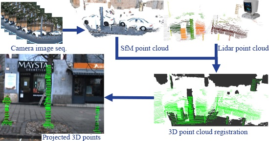
Our proposed approach is an automatic process consisting of a number of algorithmic steps for Lidar-camera sensor calibration, as presented in (Figure 1). To avoid sensitive feature matching (2/3D interest points, line and planar segments), we propose a two-stage calibration method where first we use a Structure from Motion (SfM) [21] based approach to generate a 3D point cloud from the consecutive image frames recorded by the moving vehicle (see Figure 2). In such manner, the calibration task can be defined as a point cloud registration problem. Then, a robust object-based coarse alignment method [22] is adopted to estimate an initial translation and rotation between the Lidar point cloud and the synthesized 3D SfM data. In this step, connected point cloud components called abstract objects are extracted first, followed by the calculation of the best object level overlap between the Lidar and the synthesized SfM point clouds, based on the extracted object centers. A great advantage of the method is that although the number of the extracted object centers can be different in the two point clouds, the approach is still able to estimate a robust transformation. Following the coarse initial transformation estimation step we decrease the registration error using the Iterated Closest Point (ICP) point level method. Thereafter, to compensate the effects of the non-linear local distortions of the point clouds (SfM errors, and shape artifacts due to platform motion), we introduce a novel elastic registration refinement transform, which is based on non-uniform rational basis spline (NURBS) approximation (see details later). Finally, we approximate the 3D–2D transformation between the Lidar points and the corresponding image pixels by an optimal linear homogeneous coordinate transform.

In our experiments, we observed a common problem that in SfM point clouds, dynamic objects such as vehicles and pedestrians often fall apart into several blobs due to several occlusions and artifacts during the SfM processing. This phenomenon significantly reduced the performance and robustness of the matching. To handle this issue we introduce a pre-processing step: before the coarse alignment we eliminate the dynamic objects both from the Lidar and the synthesized SfM point cloud data by applying state-of-the-art object detectors. We use Mask R-CNN [23] to provide an instance level semantic segmentation on images, while the Point pillars method [24] to detect dynamic objects in the Lidar point cloud.

As output, the proposed approach provides a $4\times 3$$\widehat{T}$ matrix which represents an optimized linear homogeneous transform between the corresponding 3D Lidar points and the 2D image pixels. To generate $\widehat{T}$, our algorithm calculates three matrices ($T_1$, $T_2$ and $T_3$) and a non-rigid transformation (${\mathcal{T}}_{★}$): The first matrix, $T_1$ is calculated during the SfM point cloud synthesis, and it represents the (3D-2D) projection transformation between the synthesized SfM point cloud and the first image of the given image sequence which was used to create the SfM point cloud. Hence matrix $T_1$ can be used to project the synthesized 3D points to the corresponding pixel coordinates of the images. Matrix $T_2$ represents the coarse rigid transform (composed by a translation and rotation components) between the Lidar and SfM point clouds, estimated by the object level alignment step, while $T_3$ is the output of the ICP-based registration refinement. The non-rigid body transformation ${\mathcal{T}}_{★}$ scales and deforms the local point cloud parts compensating the distortion effects of the SfM and Lidar point cloud synthesis processes. Finally, we approximate the cascade of the obtained transforms $T_1$, $T_2$, $T_3$, ${\mathcal{T}}_{★}$ with a single global homogeneous linear coordinate transform $\widehat{T}$, using the EPnP [25] algorithm:

$$(T_1,T_2,T_3,{\mathcal{T}}_{★})\stackrel{\mathrm{EPnP}}{\to }\widehat{T}.$$

(1)

Note that we will also refer to the composition of the two 3D–3D rigid transform components as $T_R=T_2·T_3$. The steps of the proposed approach are detailed in the following subsections.

3.1. Structure from Motion (SfM)

As a first step, we generate a 3D synthesized point cloud from consecutive camera frames reinterpreting the calibration task as a point cloud registration problem. To generate the synthesized SfM point clouds we modified and extended the SfM pipeline [21] from the OpenMVG (Url: https://github.com/openMVG/openMVG) library [26] which we describe in the following.

To generate the synthesized point cloud, we start capturing $1288\times 964$ pixel sized image frames and we select a set of N ($N\ge 3$) images ($N=8$ is used in this paper). We include the current frame among the N frames to be processed if there exists a global movement of at least $t{h}_{move}\ge 10$ pixels between consecutive frames. After gathering the N frames, we execute the following steps:

• Image rectification: First we rectify the selected images (Figure 2a) using the intrinsic camera parameters.
• Semantic segmentation: Using a state-of-the-art instance level segmentation approach called Mask R-CNN [23] we label the dynamic objects (Figure 3a) such as vehicles and pedestrians on the rectified frames.
• Consecutive frame correspondences: $L_2$ fast cascade matching is used to match the extracted SIFT feature points between the consecutive frames.
• Structure from motion calculation: In this step we perform a SfM pipeline to generate a sparse point cloud (Figure 2b) from the selected image sequence and we also store the 2D image pixel coordinates (Figure 4) from all images that contributed to the calculation of the current 3D points. We assign unique IDs to all 2D interest points in all images and propagate the point IDs through the SfM pipeline along with the associated Mark R-CNN semantic segmentation labels into the generated point cloud. Thus, we will know which 2D points from which frames contributed to the calculation of each 3D point in the produced point cloud. (Figure 3b).
• Transformation calculation: Based on point density we select M points (in this paper $M=45$ and the point labels cannot be dynamic objects) from each processed frame and using the stored 3D-2D point correspondences (Figure 4a,b). We apply the EPnP [25] algorithm to estimate a transformation matrix $T_1$ of Equation (1) which is able to project the 3D points onto the corresponding 2D image pixels. Note that different $T_1$ matrices belong to every frame of the N images used to create the SfM point cloud. In practice, we calculate $T_1$ only for a single frame, selected via time stamp comparison with the actual Lidar point cloud. To validate if the estimated projection matrix is correct, we re-project the 3D points to the corresponding images (Figure 4c) and we calculate the re-projection error based on the stored 3D-2D point associations. Using our method, we measured $1.02$ pixel error in average which we determined to be enough empirically to achieve a robust calibration result.
• Sparse point cloud densification: Figure 2c demonstrates the result of the densification step by using the PatchMatch [27] algorithm from OpenMVS (Url: http://cdcseacave.github.io/openMVS) library without any modification. We use the densified point cloud (Figure 2c) and the estimated projection matrix in the next steps of the proposed approach.

Since our modified SfM pipeline can be performed on-the-fly, during the data capturing process we can periodically calculate the synthesized dense SfM point cloud from selected N consecutive frames. Thus, the method can efficiently operate on experimental test platforms, where the movements of the vehicle may cause some displacements of the temporarily fixed sensors. Note that even industrial sensor configurations may need re-calibration at specific time intervals, which is also straightforward using our technique, since to perform our whole pipeline takes about 2–3 min (using an Intel Core i7 Coffee Lake processor), and it is not required to stop driving or using any calibration targets.

3.2. Point Cloud Registration

In the next phase of the proposed algorithm, we aim to transform the Lidar point cloud and the previously synthetized SfM point cloud (Section 3.1) to the same coordinate system.

Several point level registration methods can be found in the literature. Many of them are variants or extensions of the classical iterative ICP or the Normal Distributions Transform (NDT) [28] methods, which often fail if the initial translation is large between the point clouds. In addition, they are usually inefficient when the density characteristics of the two point clouds are quite different, furthermore the typical ring patterns of RMB Lidar data may mislead the registration process by finding irrelevant correspondences on the ground level instead of finding associations between the foreground regions [17]. In order to avoid such registration artifacts, we proposed an object level point cloud alignment approach [22] to estimate an initial translation and rotation between the point clouds.

We found that since the proposed SfM (Section 3.1) pipeline operates on image sequences of $N=8$ frames, the global diameter of the generated SfM model is usually much smaller than the diameter of the recorded RMB Lidar point cloud. Therefore, to facilitate the registration, in the further processing steps we only consider the central segment of the Lidar measurement with a 15 m radius around the sensor position.

3.2.1. Object Detection

Instead of extracting local feature correspondences from the global scene, we detect and match various landmark objects in the SfM-based and the Lidar point clouds. In the next step based on the landmark object locations we estimate the transform which provides the best overlap between the two object sets.

As a preprocessing step, we first detect the dynamic object regions which can mislead the alignment, thus it is preferred to remove their regions before the matching step. On the one hand, based on the predicted semantic labels in the camera images (Section 3.1), we determine the camera-based 3D locations of the vehicles and pedestrians by projecting the 2D labels to the synthesized 3D SfM point cloud (see Figure 3). On the other hand, to eliminate the dynamic objects from the Lidar point cloud we adopt a state-of-the-art object detector called Point pillars [24] (see Figure 5b), which takes the full point cloud as input and provides bounding box candidates for vehicles and pedestrians. As a result of the filtering, during the subsequent alignment estimation we can rely on more compact and robustly detectable static scene objects such as columns, tree trunks and different street furniture elements.

After the dynamic object filtering step we also remove the ground/road regions by applying a spatially adaptive terrain filter [17], then we extract connected component blobs (objects) from both the synthesized SfM and the Lidar point clouds.

Euclidean point distance based clustering methods are often used to extract object candidates from point clouds, for example [29] used kD-tree and Octree space partition structures to efficiently find neighboring points during the clustering process. However these methods often yield invalid objects, either by merging nearby entities to large blobs, or by over-segmenting the scene and cutting the objects into several parts. Furthermore, building the partition tree data structure frame by frame causes noticeable computational overload. Börcs et al. [30] proposed an efficient 2D pillar-structure to robustly extract object candidates using a standard connected component algorithm on a two level hierarchical 2D occupancy grid, however that method erroneously merges multiple objects above the same 2D cell even if they have different elevation values (such as hanging tree crowns).

To handle the merging problem of the 2D grid based approaches alongside the height dimension we propose an efficient sparse voxel structure (SVS) to extract connected components called abstract objects from the point cloud data (Figure 6d,e). While using only the pillar structure, which is similar to a traditional 2D grid approach [30], the objects may be merged alongside the height dimension (see Figure 6d), in a second step focusing on the vertical point distribution we can split the erroneously merged regions using the voxel level representation of the SVS (see Figure 6e).

The most elementary building block of the SVS is the voxel (see Figure 6a) which is a cube volume of the 3D space containing a local part of the given point cloud. Furthermore the vertically aligned voxels form a so called pillar structure (see Figure 6b) which is an extension of the voxels to be able to operate as a simple 2D grid similarly to [30]. Creating a fully dense voxel model based on the bounding box dimensions of the point cloud is quite inefficient, since in a typical urban environment only a few segments of the bounding space contain 3D points. To ensure memory efficiency for our SVS, we only create a voxel if we find any data point in the corresponding volume segment. In our case, the average size of the point cloud bounding boxes is around $30\times 30\times 5$ m, and we found that the optimal voxel resolution for object separation in a typical urban environment is $0.2$ m [30]. While in this case a full voxel model would require the management of around 562,500 voxels, our proposed SVS usually contains less than 30,000 voxels, which yields a great memory and computational gain, while efficient neighborhood search can be maintained with dynamically created links within the new data structure. Note that we can find alternative sparse voxel structures in the literature such as [31,32], however those methods are based on Octree structures, and they were designed for computer graphics related tasks such as ray tracing. On the other hand our SVS fully exploits the fact that in an urban environment most of the objects are horizontally distributed along the road, while vertical object occlusions are significantly less frequent.

Next, we describe the object extraction process using our SVS. First, similarly to [30] we detect the ground regions using a spatially adaptive terrain filtering technique. Second, using the pillars structure of the SVS, we can quickly extract connected components (objects) by merging the neighboring pillars into object candidates. Third, considering the voxel level resolution of the SVS, we separate the erroneously merged blobs along the height dimension.

After the extraction of abstract objects, we assign different attributes to them, which will constraint the subsequent object matching steps (Section 3.2.2). We calculate the following three attributes for each object blob o:

• Centroid ($o.c$): The center of mass of the local point cloud belonging to the object.
• Bounding box ($o.b$): minimal and maximal point coordinate values along each dimension.
• Shape category ($o.s$): we assign to each object the shape category linear, flat or scattered object (see Figure 6c).

The assigned shape category is based on a preliminary voxel level segmentation of the scene (see Figure 7). For each voxel, we determine a linearity and a flatness descriptor, by calculating the principal components and the eigen values $({\lambda }_1\ge {\lambda }_2\ge {\lambda }_3)$ of the point set in the voxel, using the Principal Components Analysis (PCA) algorithm. By examining the variance in each direction, we can determine the linearity and flatness properties as follows [33]:

$$\begin{array}{cc}\hfill \left(1\right)Linearity& =\frac{{\lambda }_1}{{\lambda }_1+{\lambda }_2+{\lambda }_3}\hfill \\ \hfill \left(2\right)Flatness& =1-\frac{{\lambda }_3}{{\lambda }_1+{\lambda }_2+{\lambda }_3}\hfill \end{array}$$

• If ${\lambda }_1$ is large (${\lambda }_1>0.7$) compared to the other two eigenvalues, it means that the included points lie on a line, so the voxel is part of a linear structure such as pole or wire.
• If the total variance is defined by the two largest eigenvalues that means points lie on a plane.
• If $Flatness>0.6$ the voxel is classified as flat voxel. Typically wall segments and parts of larger objects are built from flat voxels.
• Unstructured regions can also be detected using the third eigenvalues. If ${\lambda }_3>0.1$ that means point scattering is high in the region. Vegetation and noise can be detected efficiently using this property.

Note that the above threshold values should be empirically defined, since they depend on the characteristics of the given point cloud. Following the guidelines of [33], we fine-tuned the threshold parameters based on our experiments. Figure 6c demonstrates the voxel level classification based on the linearity and flatness values. Finally, for each extracted abstract object we determine its shape category by a majority voting of its included voxels.

3.2.2. Object Based Alignment

At this point, our aim is to estimate a sufficient initial alignment between the synthesized SfM and Lidar point clouds based on the above detected abstract objects (Figure 7). In order to find the optimal matching, we use the extracted two sets of object centroids from the SfM-based and the Lidar point clouds, respectively, and we search for an optimal rigid transform, $T_2$ of Equation (1), between the two point sets by an iterative voting process in the Hough space [22]. We observed that the search for the translation component of the transform can be limited to a 15m radius search area (which is equal to the base size of the considered point cloud segments), while it is also crucial to roughly estimate the rotation component around the upwards axis. On the other hand, the other two rotation components are negligible, as the road elevation is usually quite short within the local road segments covered by the considered point clouds, thus the minor rotation errors caused by ignoring them can be corrected later through point level transformation refinement.

Estimation of the proper 3D translation vector $(dx,dy,dz)$ among the three coordinate axes and the $\alpha$ rotation value around the upwards axis is equivalent to finding an optimal 3D rigid body transformation in the following form:

$$T_{dx,dy,dz,\alpha }\left(\begin{array}{c}x\\ y\\ z\\ 1\end{array}\right)=\left[\begin{array}{cccc}cos\alpha & sin\alpha & 0& dx\\ -sin\alpha & cos\alpha & 0& dy\\ 0& 0& 1& dz\\ 0& 0& 0& 1\end{array}\right]\left[\begin{array}{c}x\\ y\\ z\\ 1\end{array}\right]$$

The above transformation estimation can be defined as a finite search problem by discretization of the possible parameter space into equal bins. Considering that our transformation has four degrees of freedom (3D translation vector and a rotation component around the upwards axis) we allocate a 4D accumulator array $A[\alpha ,d_x,d_y,d_z]$.

Let us denote the abstract object sets extracted from the SfM and the Lidar point clouds by $C1$ and $C2$ respectively. During the assignment, we attempt to match all possible $o1\in C1$ and $o2\in C2$ object pairs, however to speed up the process and increase its robustness we also introduce a compatibility measurement between the objects. As discussed in Section 3.2.1, during the object detection step we assigned a bounding box ($o.b$) and a shape category ($o.s$) parameter to each extracted abstract object. We say that $o1\in C1$ and $o2\in C2$ are compatible, if the side length ratios of their bounding boxes are between predefined values ($0.7\le \frac{o1.b_x}{o2.b_x},\frac{o1.b_y}{o2.b_y},\frac{o1.b_z}{o2.b_z}\le 1.4$) and their shape categories are the same ($o1.s=o2.s$).

Algorithm 1 shows the pseudo code of the proposed object-based alignment algorithm. The approach iterates through all the compatible $o1\in C1$ and $o2\in C2$ object pairs and it rotates $o2$ with all the possible $\alpha$ values. We calculate the Euclidean distance between the rotated $o{2}^{\prime }.c$ and the $o1.c$ centroid points in the following way:

$$\left[\begin{array}{c}dx\\ dy\\ dz\end{array}\right]=o1.c-\left[\begin{array}{ccc}cos\alpha & sin\alpha & 0\\ -sin\alpha & cos\alpha & 0\\ 0& 0& 1\end{array}\right]o2.c$$

(2)

Algorithm 1 Object-based point cloud alignment. Input: two point clouds $F1$ and $F2$, output: the estimated $TR=T_R$ rigid transformation between them. $Rot\left(\alpha \right)$ denotes a rotation matrix around the upwards axis.

1: procedureAlignment($F1$, $F2$, $TR$) 2:     $C1\leftarrow ObjectDetect\left(F1\right)$ 3:     $C2\leftarrow ObjectDetect\left(F2\right)$ 4:     Initialize 4D accumulator array A 5:     for all $o1\in C1$ do 6:         for all $o2\in C2$ do 7:            if $iscompatible(o1,o2)$ then 8:                for $\alpha \in [0,359]$ do 9:                    $o{2}^{\prime }.c\leftarrow Rot\left(\alpha \right)\ast o2.c$ 10:                    $(dx,dy,dz)\leftarrow o1.c-o{2}^{\prime }.c$ 11:                    $A[\alpha ,dx,dy,dz]\leftarrow A[\alpha ,dx,dy,dz]+1$ 12:                end for 13:            end if 14:         end for 15:     end for 16:     $\alpha ,dx,dy\leftarrow FindMaximum\left(A\right)$ 17:     $F1,T2\leftarrow TransformCloud(F1,\alpha ,dx,dy,dz)$ 18:     $F1,T3\leftarrow ICP(F1,F2)$ 19:     $TR\leftarrow T3\ast T2$ 20: end procedure

During a given iteration step the method addresses the accumulator array with the actual $\alpha$, it calculates the corresponding $dx$, $dy$ and $dz$ translation components using Equation (2), then it increases the evidence of the transformation defined by the $(\alpha ,dx,dy,dz)$ quadruple. At the end of the iterative process, the maximal vote value in the accumulator array determines the best transformation parameters, i.e., the best $\alpha$ rotation and the $dx$, $dy$ and $dz$ translation components. Thereafter, using the estimated transformation matrix the Lidar point cloud is transformed to the coordinate system of the synthesized SfM model.

The above point cloud registration process is demonstrated in Figure 5. Note that as we mentioned in the beginning of Section 3.2.1, we aimed to restrict the object matching step to static landmark objects, therefore we first removed the vehicle and pedestrian regions from the 3D scene (see Figure 5a,b). As Figure 5c–e confirm, this step may have a direct impact on the quality of the object-based alignment algorithm: subfigure (c) shows the initial alignment of the Lidar and the SfM point clouds with a large translation error, subfigure (d) shows the result of the proposed coarse alignment algorithm without eliminating the dynamic objects from the point clouds in advance, while subfigure (e) demonstrates the output of the proposed complete algorithm which provides a significantly improved result.

To eliminate the discretization error of the object-based alignment we can refine the estimation of the rigid transformation using a standard ICP [28] method which yields a $T_3$ matrix of Equation (1), so that the unified rigid transform between the SfM and Lidar point clouds is represented as $T_R=T_2·T_3$.

3.3. Control Curve Based Refinement

In the previous section, we estimated an optimal rigid transformation $T_R=T_2·T_3$ between the synthesized SfM model and the Lidar point cloud, which is composed of a global translation and a rotational component. However, during the SfM pipeline various artifacts may occur such as deformations due to invalid depth calculation, effects which can significantly distort the geometry of the observed 3D scene. On the other hand, due to the vehicle motion, the Lidar point clouds may also suffer from shape distortion as detailed in the Introduction. To handle the local point cloud deformation problems during the point cloud registration process, we propose a control curve based refinement method, that calculates the non-rigid ${\mathcal{T}}_{★}$ transform component of Equation (1) (see Figure 8).

To estimate the local shape deformations of the point clouds, we use the extracted object centroids as control points, and we fit separate NURBS curves to the control points of the SfM and the Lidar point clouds, respectively. As shown in Figure 8a, after the rigid body transformation based alignment there are point cloud regions which fit quite well, while in other (distorted) segments we observe significant local alignment errors.

For this reason, we introduce a non-rigid curve-based point cloud registration refinement step (see Figure 9):

• Using the extracted object centers as control points, we fit NURBS curves to the SfM and the Lidar point clouds. In Figure 9 red dots mark the control points and bluish curves demonstrate the NURBS curves. Based on the assignment results of the object-based alignment step (Section 3.2.2), we can utilize the correspondences between the control points to obtain the coherent objects pairs.
• Let us assume that based on the object alignment, the curve segments between $O_1$ and $O_2$ belong together. Between each neighboring control point pair, we subdivide the curve segment into equal bins, so that we assign the first bin of the Lidar curve segment to the first bin of the SfM curve segment.
• In the next step we assign each point of the Lidar point cloud to the closest bin of the Lidar based NURBS curve.
• Taking the advantage that a NURBS curve is locally controllable, we can transform the local parts of the Lidar point cloud separately. We calculate a translation between each corresponding bins of the SfM and Lidar based curve segments by subtracting the coordinates of the Lidar bins from the corresponding SfM bins. Since we assigned each Lidar point to one of the curve bins, we can transform these points using the translation vector of the given curve segment, which points from the given Lidar bin to the corresponding SfM bin. Since each part of the Lidar point cloud is transformed according to the corresponding curve segment, this process implements a non-rigid body transformation.

Figure 8b show the results of the curve-based registration refinement step, demonstrating a significant improvement in the initially misaligned point cloud segments.

3.4. 3D Point Projection Calculation

Our final goal is to estimate a transformation $\widehat{T}$ which is able to project the 3D points from the original coordinate system of the Lidar sensor directly to the corresponding 2D image pixels. Figure 10 demonstrates the proposed workflow of the point cloud projection. From $N=8$ consecutive image frames using an SfM pipeline we estimate a dense SfM point cloud, and we also calculate and store a unique $T_1$ projection transformation between the generated dense SFM point cloud and the original image frames. Thereafter we take the Lidar point cloud with the closest time stamp to the first frame of the actual N-frame sequence and we estimate a transformation which is able to transform the Lidar point cloud to the coordinate system of the SfM point cloud. The estimated transformation consists of a rigid body component composed by an object-based ($T_2$ ) and a point-based (ICP) term ($T_3$), as well as a NURBS-based non-rigid transform component (${\mathcal{T}}_{★}$).

Since the non-rigid body transform ${\mathcal{T}}_{★}$ cannot be defined in a closed form as a simple matrix multiplication, we calculate an approximate direct transformation between the original Lidar point cloud domain and the image pixels for preserving computational efficiency of the data fusion step. For this reason, with applying the above estimated transformation components ($T_1$, $T_2$, $T_3$ and ${\mathcal{T}}_{★}$) we project the centroid points of the extracted Lidar objects onto the camera images and we store the 3D-2D correspondences. In the next step, upon the available 3D-2D point correspondences we estimate a single homogeneous linear transformation $\widehat{T}$ which can be used to project the raw Lidar points directly to the image domain (see Figure 11). $\widehat{T}$ is calculated by the OpenCV $solvePnP$ function, which is based on the Levenberg-Marquardt optimization method [34]. As a final result, Figure 11 shows the projection of the Lidar data to the image domain.

4. Experiments and Results

To evaluate our proposed target-less and fully automatic self-calibration method we compared it to two state-of-the-art target-less techniques [4,5], and an offline target-based method [2]. We quantitatively evaluated the considered methods by measuring the magnitude and standard deviation of the pixel level projection error values both in the x and y directions along the image axes (

Table 1. Performance comparison of the target-less proposed method with two state-of-the-art target-less reference methods and with a target-based (supervised) reference technique. Notes: * Test set names Slow and Fast refer to the speed of the data acquisition platform.

Set *	Method	x-Error (pixel)		y-Error (pixel)
		Avg.	Dev.	Avg.	Dev.
Slow	Target-based ref. [2]	1.13	0.27	1.75	0.37
	Bearing angle [4]	4.56	2.15	4.58	1.74
	Line-based [5]	3.36	1.45	3.47	0.98
	Proposed	2.58	0.73	2.82	0.88
Fast	Target-based ref. [2]	3.04	0.74	2.74	0.41
	Bearing angle [4]	4.87	2.46	4.42	1.91
	Line-based [5]	5.01	1.93	4.01	1.49
	Proposed	2.84	0.95	3.14	0.82

).

We collected test data from overall 10 km long road segments in different urban scenes such as boulevards, main roads, narrow streets and large crossroads. To take into account the daily traffic changes, we recorded measurements both in rush hours in heavy traffic, and outside the peak hours as well. Since using the rotating multi-beam Lidar technology, the speed of the moving platform influences the shape of the recorded point cloud, we separately evaluated the results for measurements captured by slow and fast vehicle motion, respectively. Therefore we defined two test sets: set Slow contains sensor data captured at speed level between 5 and 30 km/h, while set Fast includes test data captured at speed above 30 km/h.

Figure 12 and Figure 13 visually demonstrate the steps of the proposed workflow.

4.1. Quantitative Evaluation and Comparison

We measured the projection error of the proposed and the reference methods by projecting the 3D Lidar points onto the 2D image pixels, which was followed by visual verification. Before starting the test, we carefully calibrated the Lidar and camera sensors using the offline target-based reference method [2], which served as a baseline calibration for the whole experiment. During our 10 km long test drive, we chose 200 different key frames of the recorded measurement sequence, and by each key frame, based on the actual a Lidar point cloud and $N=8$ consecutive camera images, we executed new calibration processes in parallel by our proposed approach and by the remaining automatic reference techniques [4,5]. We paid attention to collect these key frames from diverse scenarios (main roads, narrow streets, etc.), and we also noticed the corresponding vehicle speed values to assign each key frame either to the Slow or to the Fast test set. We evaluated the performance of all considered methods by each key frame (i.e., after each re-calibration). To calculate the pixel projection error we manually selected 10 well defined feature points (e.g., corners) from different regions of the 3D point cloud, and using the calibration results of the different methods we projected these 3D feature points to the image domain. Finally we measured the pixel errors versus the true positions of the corresponding 2D feature points positions detected (and manually verified) on the images.

As shown in Table 1, both in the Slow and Fast test sets our proposed approach notably outperforms the two target-less reference methods [4,5] in mean pixel error, and it also exhibits lower error deviation which indicates a more robust performance. Although in the Slow test set, in terms of accuracy, the proposed approach is slightly outperformed by the considered offline target-based calibration technique [2], it should be emphasized that the operational circumstances are quite different there. On one hand, according to our experiences the calibration of the camera-Lidar system using [2] takes more than two hours with several manual interaction steps, furthermore if the sensors are slightly displaced during the drive due to vibration, one must stop the measuring platform and re-calibrate the system offline. On the other hand, our proposed approach is able to calibrate the camera and Lidar on-the-fly and in a fully automatic way, even during driving without stopping the car.

We can also observe in Table 1, that in the Fast test set our proposed method can reach or even surpass the accuracy of the target-based method, since we can adaptively handle the vehicle speed dependent shape deformations of the recorded RMB Lidar point clouds. By increasing the speed of the scanning platform, we can observe that the shape of the obtained Lidar point cloud becomes distorted, and gets stretched in the direction of the movement. Since the offline, target-based method cannot re-calibrate the system during the drive, its accuracy may decline when the car accelerates. On the contrary, our proposed method is able to re-calibrate the system at different speed levels, and taking the advantage of the non-rigid transformation component, it can be better adapted to the non-linear shape distortions of the point cloud.

To quantify the improvements of the consecutive calibration steps of the proposed method, we also compared the pixel level projection errors at three different stages of our algorithm pipeline. In

Table 2. Performance evaluation of the proposed method at different calibration steps. First we measure the projection error using only the object-based coarse alignment, then we extended the method with the dynamic object filtering based on Mask R-CNN and PointPillars techniques, and finally we measure the impact of the ICP and the proposed curve-based refinement.

Step of Our Method	x-Error (pixel)		y-Error (pixel)
	Avg.	Dev.	Avg.	Dev.
Object-based alignment (OBA) on raw frames	4.78	2.26	5.21	2.47
OBA with preliminary dynamic object filtering	3.46	0.85	4.47	1.24
Final result also using ICP and NURBS-based refinement	2.58	0.73	2.83	0.88

, the first row shows the results of using the object-based coarse alignment (OBA) step on the raw Lidar frames; the second row refers to using OBA with preliminary dynamic object filtering (DOF), finally the third row displays the error parameters obtained by the complete workflow including the ICP and curve-based refinement steps. Since applying DOF can prevent us from considering several invalid object matches, we can see a large improvement in the robustness between the first and second stages, furthermore by exploiting the point level ICP and curve-based refinement steps (third stage), the projection accuracy can be significantly upgraded.

4.2. Robustness Analysis of the Proposed Method

Since our proposed method is able to re-calibrate the sensors periodically during the movement of the sensor platform, it is important to measure the robustness of the approach. We recall here that during the proposed algorithm pipeline, we already attempt to internally estimate the quality of the calibration: First following the SfM point cloud synthesis we re-project the generated point cloud to the original image pixels, and only continue the process if the re-projection error is smaller than 2 pixels. Second, following the estimation of both the rigid, and the NURBS-based non-rigid transformation components, we calculate the point level Hausdorff distance between the registered SfM and Lidar point clouds, and only accept the new calibration if the distance is lower than 5 cm. In summary, if these threshold-based constraints are not satisfied we reject to apply the current transformation estimation and we start a new calibration process.

In Section 4.1, we manually measured the errors based on 10 selected feature points in each Lidar frame. Due to the lack of availability of a Ground Truth (GT) transform [35], there is no straightforward way to extend this validation step for all points of the Lidar point cloud. However, we have performed an additional experiment to quantitatively measure the reliability and repeatability of the proposed approach. Although as discussed in Section 4.1, the target-based reference (TBR) method [2] itself may also suffer betweem one and three pixel registration errors, we observed that these errors can usually be considered constant when driving with an approximately standard average speed. Exploiting this fact, we used here TBR as a baseline technique, and we re-calibrated with 500 randomly selected seed frames the Lidar and the camera sensors using the proposed approach.

By each re-calibration step, we calculated the average point projection differences in pixels between our actual calibration and the TBR registration considering all points of the Lidar point cloud. Figure 14 shows the differences measured in pixels in the x and y directions over the subsequent calibration trials. Based on this experiment the proposed approach proved to be quite stable again, as the measured differences range between 1.2 and 1.8 pixels in the x direction, and 1.0 and 1.4 pixels in the y direction, without significant outlier values.

We also examined the impact of the roughness of discretization in the accumulator space in the voting process during the object-based registration. If we increase the step size of the $\alpha$ rotation parameter around the upward axis, or if we divide the space of the possible translation components $dx$, $dy$ and $dz$ into larger bins, we lose accuracy, however the algorithm may show an increased robustness. On the contrary, if we choose a smaller rotation step size and we increase the resolution of the possible translation space we can reach more accurate results; however, we must also expect an increasing number of unsuccessful registration attempts, as the maximum value in the voting array may become ambiguous. Based on our experiments we used an optimal rotation step size of $0.25$ degrees for $\alpha$, and an optimal resolution of $0.2$ m for the translation components $dx$, $dy$ and $dz$. These experiments are consistent with our previous observations regarding an optimal cell resolution in the case of RMB Lidar sensors [36], keeping in mind that the accuracy can be enhanced in the subsequent point level ICP step.

There can be situations when the SfM pipeline cannot produce suitable synthesized point clouds. For example, the strong sunlight may cause burnout in the images limiting the traceable features during the SfM process. However, the proposed approach is able to periodically repeat the calibration pipeline and we should only update the calibration when the current estimation improves the previously used one in terms of Hausdorff error between the SfM and Lidar point clouds. Since the object-based alignment step of the proposed approach greatly depends on the landmark candidates (objects) used for registration, we preliminary analyze the scene using the computed linearity and flatness values and the extracted bounding boxes, and we only start the calibration pipeline if the number of the proper object candidates (column shaped objects such as traffic signs, tree trunks and poles) is more than three. Typically in main roads and larger crossroads the scenes contain several column shaped landmark objects, where the proposed self-calibration algorithm works more robustly and accurately.

4.3. Implementation Details and Running Time

We implemented the proposed method using C++ and OpenGL. An NVIDIA GTX1080Ti GPU with 11 GB RAM was used to speed up the calculations. The running time of the entire calibration pipeline is less than 3 min. For data acquisition we used $1288\times 964$ resolution RGB cameras and a Velodyne HDL-64E RMB Lidar sensor.

5. Conclusions

This paper proposed a new target-less, automatic camera-Lidar calibration approach which can be performed on-the-fly, i.e., during the driving without stopping the scanning platform. Our method does not rely on any external sensors such as GNSS and IMU and we do not use hardware-based time synchronization between the Lidar and the camera. The method can periodically re-calibrate the sensors to handle small sensor displacements and it also adapts to the distortion of the RMB Lidar point cloud.

We quantitatively evaluated and compared our method to state-of-the-art target-less techniques and we proved that our approach surpasses them. Furthermore, we have shown that in some cases the proposed method even reaches the accuracy of the considered target-based reference method.